2 2 4 2 2 42 2 4 2 2 4
2 2 4 Rev Saúde Pública 2001;35(3):224-31
www.fsp.usp.br/rsp
A mathematical model for malaria
transmission relating global warming and
local socioeconomic conditions*
Modelo matemático para transmissão de
malária relacionada a aquecimento global e
condições socioeconômicas
Hyun M Yang
Departamento de Matemática Aplicada, Instituto de Matemática, Estatística e Computação Científica.Universidade Estadual de Campinas. Campinas, SP, Brasil
Correspondence to:
Hyun M. Yang
Depto. de Matemática Aplicada. IMECC, Unicamp
Caixa Postal 6065
13081-970, Campinas, SP, Brasil E-mail: [email protected]
*Supported by Fapesp (Process n. 98/2827-8).
The publication of this article was subsidied by Fapesp (Process n. 01/01661-3). Submitted on 30/6/2000. Reviewed on 16/2/2001. Approved on 26/2/2001. Keywords
Malaria, transmission.# Mathematical
models.# Greenhouse effect.#
Socioeconomic factors. Communicable disease control. Risk. – Sensitivity analysis.
Descritores
Malária, transmissão.# Modelos
matemáticos.# Efeito estufa.# Fatores
socioeconômicos. Controle de doenças transmissíveis. Risco. – Análise de sensitividade.
Abstract
Objective
Sensitivity analysis was applied to a mathematical model describing malaria transmission relating global warming and local socioeconomic conditions.
Methods
A previous compartment model was proposed to describe the overall transmission of malaria. This model was built up on several parameters and the prevalence of malaria in a community was characterized by the values assigned to them. To assess the control efforts, the model parameters can vary on broad intervals.
Results
By performing the sensitivity analysis on equilibrium points, which represent the level of malaria infection in a community, the different possible scenarios are obtained when the parameters are changed.
Conclusions
Depending on malaria risk, the efforts to control its transmission can be guided by a subset of parameters used in the mathematical model.
Resumo
Objetivo
Aplicar a análise da sensitividade ao controle de transmissão de malária a um modelo, considerando o aquecimento global e as condições socioeconômicas locais.
Métodos
O modelo para a transmissão de malária proposto foi obtido em função de vários parâmetros. A prevalência de malária, em uma comunidade, foi caracterizada pelos valores desses parâmetros. Para estudar os efeitos dos mecanismos de controle, os valores dos parâmetros do modelo são variados em grandes intervalos.
Resultados
2 2 5 2 2 5 2 2 5 2 2 5 2 2 5 Rev Saúde Pública 2001;35(3):224-31
www.fsp.usp.br/rsp
Sensitivity analysis to malaria transmission model
Yang HM
INTRODUCTION
A mathematical model was developed elsewhere8 taking into account some biological features related to malaria disease, such as partial acquired immunity, immunologic memory and duration of sporogony. From the model equilibrium points were determined and the stability of these points was analyzed. Moreover, the basic reproduction ratio related to malaria transmission was obtained. This valuable epidemiological parameter is associated with control or eradication efforts.
In a subsequent study9 the previously developed model was used to assess the effects of global warming and local socioeconomic conditions on malaria transmission. These effects were assessed analyzing the equilibrium points calculated at different but fixed values of the parameters of the model. Regarding malaria transmission, it was observed that the effects of global warming posed a major challenge in the next years,3 and the effects of variation in local socioeconomic conditions are much stronger than the effects of the increasing global temperatures.2
The epidemiological analysis was restricted to few cases taking into account a combination of the values assigned to the parameters of the model. This because the model was structured with plenty of parameters. There is another way to study this issue instead of combining a great number of parameters, whose values can vary largely. Thus, the sensitivity analysis of the model is carried out with greatly variable parameters. This analysis also provides scenarios of possible outcomes under feasible strategies of intervention.5-7
METHODS
In this section, the focus in on the model sensitivity analysis regarding the variation in the parameters of the model. In order to achieve the magnitude of impact of each parameter on the state (dynamic) variables the model and the sensitivity analysis are presented.
Initially, it is taken from Yang8 the system of differential equations which describes the overall malaria transmission. For humans, the seven compartments are: susceptible (x1), incubating, i.e., infected but non-infectious (x2), infectious (x3), immune (x4), partially immune (x5), non-immune but
with immunologic memory (x6) and incubating after reinfection (x7). The fractions of the host population are described by the following system of differential equations,
Conclusões
Dependendo-se do nível de risco de malária, as melhores formas de mecanismos de controle da transmissão de malária são dadas por um subconjunto de parâmetros do modelo.
where µ and α are the natural and differential mortality rates of human host, respectively; θ is the natural re-sistance rate against malaria; γ1-1 and γ-1 are the aver-age periods, respectively, to start the production of gametocytes and to build up an effective immune re-sponse; π1, π2 and π3 are the rates at which protective immunity, partial immunity and immunologic memory are lost, respectively; and h is the inoculation rate. The quantity y3(t) is the fraction of infectious mos-quitoes. The functions Fi(z,Ω), for i=1 to 7, z and Ω are defined below.
The mosquito population is divided into three com-partments, y1, y2 and y3, the fraction of susceptible, incubating, and infectious mosquitoes, respectively. The mosquito population is described by the following system of differential equations
where µ’ and α’ are, respectively, the natural and in-duced mortality rates of the mosquitoes, ρ-1(T) is the
duration of sporogony in the mosquito, and f is the transmission rate. The temperature, designed by sym-bol T, was limited and was dependent only to the pa-rameter ρ. The functions Fi(z,Ω), for i=8 to 10, z and Ω are defined below.
2 2 6 2 2 62 2 6 2 2 6
2 2 6 Rev Saúde Pública 2001;35(3):224-31
www.fsp.usp.br/rsp Sensitivity analysis to malaria transmission model
Yang HM
is slightly different from the equation in Yang’s model,8 it was obtained by applying the relation
for the vector population and host population, there are
The parameters φ and µe(T) are, respectively, the rates of oviposition and of eggs becoming non-via-ble, and ρ1-1(T) is the duration of the cycle from the
egg to the mature adult. The overall model is un-changed. Therefore, µ’ and α’ should also depend on the temperature.
Defining the functions Fi(z,Ω), z and Ω. The func-tions Fi(z,Ω), for i=1,2,…,10, are the elements of the vector F(z,Ω), which are the state equations of the model. The state variables space z and parameters space Ω are given, respectively, by the vectors
and
The superscript Tr stands for the transposition of the matrix.
Depending on the value of the basic reproduction ratioR0, which is given by
the trivial or non-trivial equilibrium point is the atractor.8 If R0≤1, then the trivial equilibrium point is stable, oth-erwise the non-trivial equilibrium is stable.
The trivial equilibrium point, which represents a dis-ease-free community, is given by
for the vector population, and
for the host population.
The non-trivial equilibrium point, which represents malaria at an endemic level in a community, is given by
plus a third degree polynomial to determine x3, which is given by
The auxiliary variables b1, b2, b3, b4, b5, c1 and c2, and the coefficients of the polynomial A, B, C and D can be found in Yang’s study.8
The sensitivity analysis provides the range of vari-ation of the model’s variables, such as state variables and basic reproduction ratio, when the values of the parameters of the model are changed. The state vari-ables in the equilibrium, which are given by the equa-tions (4) and (5), when trivial, and by the equaequa-tions (6), (7) and (8), when non-trivial, and the basic re-production ratio, which is given by the equation (3), are dependent on the parameters of the model. Since the parameters of the model are not accurate, it is expected that the variables of the model be influence by the inaccuracy of those values. On the other hand, if it is possible to change few parameters with an appropriate intervention, it is interesting to know what parameters should be changed in order to get the bet-ter results. Both issues can be addressed applying the sensitivity analysis.
First, the sensitivity analysis for the basic repro-duction ratio can be performed using equation (3). Note that the basic reproduction ratio does not de-pend on all parameters defined in Ω, for this reason the subset Ω’ of Ω is defined, given by
2 2 7 2 2 7 2 2 7 2 2 7 2 2 7 Rev Saúde Pública 2001;35(3):224-31
www.fsp.usp.br/rsp
Sensitivity analysis to malaria transmission model
Yang HM
The variation in R0, due to the inaccuracy in the values of the parameters given in Ω’, can be meas-ured by
This expression provides the contribution of each parameter, given by (hij)2(σΘ)2, with Θ=Ωj, to the
variance of the dynamic variables.
To obtain useful epidemiological information, the actual values for the parameters of the model should be known. Since their values can vary largely, Table 1 shows the range and the mean value that the average periods can assume and the corresponding rates and the standard deviations.
As can be noted, the above table was obtained from the literature for the parameters θ, γ1, γ, π1, π2, π3, µ, µ’ and ρ(T). Concerning the differential (α) and induced (α’) mortality rates, it is assumed a decrease of about 2% and 6%, respectively, in the expected life span.
Table 1 presents the parameters of the model in terms of average periods (as the arithmetic mean between the maximum and the minimum values) and their inverses, which are the rates. Let’s call, in general, the average periods as p and the rates as r. The standard deviations related to the parameter p, designed by σp,
were calculated as the half between the maximum and the minimum values that one parameter can assume. where (σΘ)2, with Θ=Ω
j’ and j=1 to 8, are the
variances given by the matrix VΩ’ considered diago-nal, and hj, with j=1 to 8, are the elements of the
vec-tor H ’given by
Observe that (hj)2(σΘ)2 is the contribution of the j-th
parameter to the variance of R0.
Second, the sensitivity analysis of the state vari-ables at equilibrium can be run by considering the state equations F(z,Ω) of the model instead of the equations (4) through (8), which provide the trivial and non-trivial equilibrium points. Using the abso-lute sensitivity function1 for the covariance matrix V
z of the state variables z,
where VΩ is the covariance matrix for the 11 param-eters of Ω stated above and H is the sensitivity ma-trix given by
with its elements denoted by hij, with i=1 to 10 and j=1 to 11. Note that the matrix P is given by
where the index 1 refers to the trivial and 2 to the non-trivial equilibrium points, and
is the Jacobian matrix. Both matrices should be evalu-ated at the equilibrium points z1 and z2. Observe that F
I (z,Ω), where i=1 to 10, corresponds to the second member of the system of equations (1) and (2).
If the covariance matrix VΩ is considered a diagonal
matrix, with its diagonal elements given by (σΘ),2 with Θ=Ωj, where j=1 to 11, then the variance related
to the state variables (the diagonal elements of Vz) are given by
Table 1 - The values found in the literature for the model’s parameters. The symbols d and y stand, respectively, for days and
years.
Parameter Range (in period) Average period Rate Standard deviation
θ (d) 1–4 2.5 0.4 0.24
γ1 (d) 15–19 17 0.059 0.007
γ (d) 50–150 100 0.01 0.005
π1 (d) 40–60 50 0.02 0.004
π2 (y) 0.2–5 2.6 0.38 0.35
π3 (y) 1–20 10.5 0.095 0.086
µ (y) 50–55 52.5 0.019 0.0009
α (y) 2450–2964 2707 0.0004 0.00004
µ’ (d) 10–14 12 0.083 0.014
α’ (d) 98–191.8 144.9 0.007 0.002
2 2 8 2 2 82 2 8 2 2 8
2 2 8 Rev Saúde Pública 2001;35(3):224-31
www.fsp.usp.br/rsp Sensitivity analysis to malaria transmission model
Yang HM
The average periods and their standard deviations should be transformed according to
since the model includes rates.
The focus is on the sensitivity analysis of a ma-thematical model for malaria transmission, consi-dering temperature change and local socioeconomic conditions. For this reason, temperature-independent parameters θ, γ1, γ, π1, π2 and π3 are
considered here as being associated roughly and indirectly to the general local socioeconomic conditions. And, evidently, temperature-dependent parameters ρ, µ’ and α’ are considered here as being associated to temperature changes.9 Also, three representative risk areas for malaria are considered by assigning particular values for the inoculation h and transmission f rates.
In the next section, based on the above values for the parameters of the model, the sensitivity analysis was performed to assess control efforts to malaria transmission. It is noteworthy, however, that the sensitivity is fundamentally a local analysis, therefore the discussion below is valid only for the above range of the values for the parameters of the model and transmission rates.
RESULTS
In this section control efforts to malaria transmission are assessed considering a mathematical model developed with different levels of acquired immunity among human hosts and the impact of temperature on the parameters associated with vectors. Sensitivity analysis is used to this assessment, taking into account the values for the parameters of the model presented in Table 1 and three representative transmission rates (given in days-1): h=0.18 and f=0.12, h=0.70 and f=0.19
and h=2.0 and f=0.26. The three couple of transmission rates focus three representative regions of malaria transmission: a low endemic area (for example, the Amazon), an intermediate endemic area (South East Asia) and a high endemic area (Africa).
Table 2 summarizes the equilibrium values calculated with the mean values of the parameters showed in the fourth column of Table 1, taking into account three transmission rates (days-1): h=0.18 and f=0.12 (Region I), h=0.70 and f=0.19 (Region II), and h=2.0 and f=0.26 (Region III).
The corresponding basic reproduction ratio are: R0=1.3 (Region I), R0=8.0 (Region II), and R0=31.23 (Region III). Note that the fractions of infectious humans (x3) and mosquitoes (y3), together with the fraction of incubating humans (x2), are reduced in Region III in comparison with Region II. Therefore, a high level of malaria transmission prevents in some extent the serious malaria disease because the fractions x2 and x3 are decreased by increasing the fractions of immune (x4) and partially immune (x5) individuals.
The sensitivity analysis was run for the basic reproduction ratio and the equilibrium values in relation to the variation in the values of the parameters of the model.
First, the variation in the basic reproduction ratio was analyzed when parameters can vary. The sensitivity analysis of the basic reproduction ratio regarding the parameters given in the space of parameters Ω’ can be performed with equation (9). This equation takes into account the contributions of each parameter to the variance of the basic reproduction ratio. In Table 3 the sensitivity analysis of R0 for the Regions I, II and III is showed.
Table 2 - The equilibrium values (in fractions) for human and
mosquito populations for Regions I, II and III calculated with values given in Table 1.
State variable Region I Region II Region III
x1 0.776 0.129 0.033
x2 0.0009 0.002 0.0015
x3 0.0052 0.0125 0.009
x4 0.0046 0.165 0.423
x5 0.0565 0.378 0.39
x6 0.156 0.308 0.14
x7 0.0002 0.005 0.006
y1 0.993 0.974 0.976
y2 0.004 0.015 0.014
y3 0.003 0.011 0.010
Table 3 - The sensitivity analysis of the basic reproduction
ratio for the Regions I, II and III considering the values given in Table 1.
Rank (parameter) Region I Region II Region III
1 (θ) 0.46 17.4 266.7
2 (γ) 0.42 15.8 241.2
3 (ρ) 0.12 4.95 70.2
4 (µ’) 0.10 3.75 57.3
5 (γ1) 0.02 0.67 10.3
6 (α’) 0.003 0.10 1.48
7 (µ) 10-7 10-6 10-4
8 (α) 10-13 10-12 10-11
Sum of variance 1.12 42.3 647.2
2 2 9 2 2 9 2 2 9 2 2 9 2 2 9 Rev Saúde Pública 2001;35(3):224-31
www.fsp.usp.br/rsp
Sensitivity analysis to malaria transmission model
Yang HM
Table 3 shows that 98.2% of the variation in R0 is due to three parameters which are related to the state variables x3 and y3, plus the mortality rate of the vector population µ’. Note that the two most sensitive (together they contribute to 78.6%) human-related parameters θ and γ are the natural resistance rate and period of time to build up the effective immunity, respectively; and the third and fourth most sensitive (together they contribute to 19.6 %) are vector-related parameters ρ, which is the duration of sporogony, and µ’. The vital dynamics parameters α and µ related to human population are practically insensitive, and the sensitivity of the input rate γ
1 to the infectious
individuals x3 and additional mortality rate of latent and infectious mosquitoes α’ are negligible.
Based on the sensitivity analysis of R0 regarding the eight parameters, the following results can be drawn. To reduce the risk of malaria infection, simplistically considering only decreasing in R0, the most effective efforts are those related to the preven-tion of the increase in the fracpreven-tions of infectious individuals x3 and mosquitoes y3. Observe that there are two mechanisms to decrease the number of infectious individuals: increasing the natural resistance rate (drug treatment) or decreasing the period of time to build up immunity (vaccination). Regarding the vector population, control efforts should increase the duration of sporogony (avoiding global warming due to pollution effects) and/or increase the mortality rate (insecticide use). Nevertheless, control efforts directed to human population are not only much more efficient but realistic than those ones directed to vectors.
Second, the variation in the equilibrium points (state variables) is analyzed with the variation in the values of the parameters of the model. The sensitivity analysis of the equilibrium points in relation to the space of parameters Ω can be carried out with equation (10). This equation takes into account the contributions of each parameter to the variance of coordinates of the equilibrium point. The Jacobian matrix J evaluated at the equilibrium point
Table 4 - The sensitivity analysis of the equilibrium point for the Region I considering the values given in Table 1. The ranking of the contribution of the parameters is based on the x1; if the ranking changes, this is set between parenthesis. The exponent between parenthesis in the first row is the multiplying factor of the entire column.
Rank (Par.) x1 (10-3) x 2 (10
-8) x 3 (10
-6) x
4 (10
-6) x
5 (10 -4) x
6 (10
-3) x
7 (10 -9) y
1 (10 -2) y
2 (10 -7) y
3 (10 -7)
1 (θ) 26.9 38.5 23.6 (ρ) 34.0 (ρ) 22.8 11.5 92.3 (ρ) 14.6 (γ) 37.8 (ρ) 85.1 (ρ)
2 (ρ) 24.2 36.9 20.0 (γ) 20.0 (θ) 19.9 (π2) 8.71 81.6 (θ) 9.59 (θ) 35.2 (γ) 19.2 (γ)
3 (γ) 7.65 10.4 13.2 (θ) 7.39 15.1 (ρ) 6.90 (π3) 22.0 3.26 (µ’) 23.2 (θ) 12.6 (θ)
4 (π3) 5.62 4.71 (µ’) 1.26 4.71 (µ’) 6.09 (γ) 3.04 (γ) 11.8 (µ’) 0.92 11.8 (µ’) 4.24 (µ’)
5 (µ’) 4.82 3.69 (π3) 0.75 0.83 (π1) 3.01 1.21 5.48 (π3) 0.39 (ρ) 2.22 (π3) 1.21 (π3)
6 (γ1) 1.03 0.42 (π2) 0.51 0.77 0.88 0.44 1.22 0.37 0.89 0.48
7 (π2) 0.64 0.12 (α’) 0.14 0.70 0.38 (π3) 0.39 0.88 0.10 0.30 (α’) 0.14
8 (α’) 0.12 0.03 (γ1) 0.02 0.47 (π3) 0.08 0.03 0.30 0.08 0.25 (π2) 0.11
9 (µ) 10-3 10-3 10-4 0.12 (α’) 10-4 (π
1) 10
-3 10-3 10-4 10-4 10-4
10 (π1) 10-4 10-4 10-5 10-5 (µ) 10-5 (µ) 10-4 10-4 10-5 10-5 10-5
11 (α) 10-12 10-11 10-12 10-12 10-12 10-12 10-12 10-12 10-12 10-13
Sum of var. 71.0 94.7 59.5 69.0 68.3 32.2 215.6 29.3 111.6 123.1
can be inverted by the Gauss-Jordan method.4
First, a very low endemic area of malaria (Region I) is considered. Table 4 shows the sensitivity analysis of the state variables for h=0.18 and f=0.12 (days-1).
Standard deviations for the state variables x1, x2, x3, x4, x5, x6, x7, y1, y2 and y3 are 0.27, 0.001, 0.0077, 0.008, 0.08, 0.18, 0.0004, 0.54, 0.0033, and 0.0035, respectively.
When a community lives in an area of very low risk of malaria, the parameters ρ, θ and γ in general are the most sensitive ones for all state variables. The times these three parameters appear leading the ranking in relation to the state variables are 5, 4 and 1, respectively. At fourth and fifth ranking comes µ’ and π3. In general, these five parameters nearly contribute with all the variations in the state variables. On the other hand, µ, π1 and α are the least sensitive parameters. Other parameters for immunity decline π2 and π3 are also less sensitive. In this scenario, susceptible individuals can reach unity value, that is, the population can be disease-free.
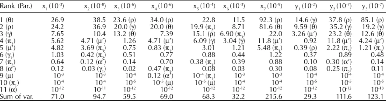
An intermediate endemic malaria area (Region II) is considered. Table 5 shows the sensitivity analysis of the state variables for h=0.70 and f=0.19 (days-1).
The standard deviations for the state variables x1, x2, x3, x4, x5, x6, x7, y1, y2 and y3 are 0.08, 0.001, 0.0074, 0.102, 0.14, 0.16, 0.004, 0.43, 0.011 and 0.007, respectively.
2 3 0 2 3 02 3 0 2 3 0
2 3 0 Rev Saúde Pública 2001;35(3):224-31
www.fsp.usp.br/rsp Sensitivity analysis to malaria transmission model
Yang HM
Table 5 - The sensitivity analysis of the equilibrium point for the Region II considering the values given in Table 1. The ranking of the contribution of the parameters is based on the x1; if the ranking changes, this is set between parenthesis. The exponent between parenthesis in the first row is the multiplying factor of the entire column.
Rank (Par.) x1 (10-4) x 2 (10
-8) x 3 (10
-6) x 4 (10
-4) x
5 (10 -3) x
6 (10
-3) x
7 (10 -6) y
1 (10 -2) y
2 (10 -6) y
3 (10 -6)
1 (γ) 31.5 60.2 (π3) 26.6 44.2 12.3 (π2) 10.5 (π3) 13.9 (π2) 11.1 (µ’) 35.5 (π2) 19.4 (π2) 2 (θ) 19.8 21.5 (π2) 20.6 (π3) 34.3 (π3) 4.30 9.97 (π2) 1.66 3.31 (π2) 26.8 (γ) 14.7 (γ) 3 (ρ) 9.68 7.09 (γ1) 7.36 (π2) 9.68 1.31 (γ) 2.75 (γ) 0.86 (γ) 2.97 (θ) 20.8 (π3) 11.4 (π3) 4 (π2) 5.76 3.34 (γ) 0.23 (ρ) 7.95 1.02 (π3) 0.97 (ρ) 0.24 (ρ) 0.35 (γ) 15.1 (ρ) 4.89 (θ) 5 (µ’) 1.93 1.48 (ρ) 0.10 (θ) 7.52 (π1) 0.97 (ρ) 0.46 (θ) 0.10 (γ1) 0.29 (α’) 12.1 3.78 (ρ)
6 (γ1) 1.07 0.31 (θ) 0.07 (π1) 0.04 0.21 0.12 (π1) 0.05 (µ’) 0.27 (π3) 8.95 (θ) 0.10
7 (π3) 0.48 0.21 (π1) 0.02 (µ) 0.03 (µ) 0.19 (µ’) 0.05 (µ’) 0.03 (π1) 0.05 (γ1) 0.31 (α’) 0.01 (µ)
8 (π1) 0.08 0.07 (µ’) 0.01 (γ1) 10-3 (θ) 0.17 0.03 (γ
1) 0.02 (π3) 0.05 0.19 (γ1) 10
-4
9 (α’) 0.05 0.06 (µ) 10-13 (α) 10-13 (α) 10-3 0.01 (µ) 10-3 10-4 (µ) 0.02 (µ) 10-14 (α) 10 (µ) 10-4 10-3 (α’) 0 (µ’) 0 (µ’) 10-4 10-3 (α’) 10-4 10-14 (α) 10-4 (π
1) 0 (µ’)
11 (α) 10-11 10-13 0 (α’) 0 (α’) 10-13 10-14 10-14 0 (ρ) 10-14 0 (α’)
Sum of var. 70.3 94.2 55.0 103.7 20.5 24.9 16.9 18.4 119.8 54.2
and α’ are the least sensitive parameters. In one occasion ρ reveals to as the least sensitive parameter.
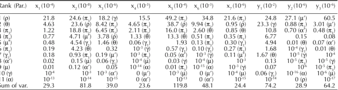
Finally, a very high endemic malaria area (Region III) is considered. Table 6 shows the sensitivity analysis of the state variables for h=2.0 and f=0.26 (days-1).
The standard deviations for the state variables x1, x2, x3, x4, x5, x6, x7, y1, y2 and y3 are 0.05, 0.001, 0.006, 0.15, 0.11, 0.22, 0.005, 0.86, 0.0053 and 0.008, respectively.
When a community lives in an area of very high risk of malaria, the parameters ρ, π2 and π3 in general are the most sensitive parameters for all state variables. The times these three parameters appear leading the ranking in relation to the state variables are, 5, 2 and 1, respectively. In one occasion µ’ and γ appear as the most sensitive parameters. At fourth and fifth ranking appear θ and γ. In general, these five parameters contribute nearly with all the variations in the state variables. On the other hand, µ, µ’ and α’ are the least sensitive parameters. In one occasion ρ appears as the least sensitive parameter.
From Tables 4, 5 and 6 it can be noted that loss of immunity parameters (π1, π2 and π3) increase their
Table 6 - The sensitivity analysis of the equilibrium point for the Region III considering the values given in Table 1. The ranking
of the contribution of the parameters is based on the x1; if the ranking changes, this is set between parenthesis. The exponent between parenthesis in the first row is the multiplying factor of the entire column.
Rank (Par.) x1 (10-4) x 2 (10
-8) x 3 (10
-6) x
4 (10
-3) x
5 (10 -4) x
6 (10
-3) x
7 (10 -6) y
1 (10 -2) y
2 (10 -6) y
3 (10 -6)
1 (ρ) 21.8 24.6 (π3) 18.2 (γ) 15.5 49.2 (π2) 34.8 21.6 (π2) 24.8 27.1 (µ’) 60.5
2 (θ) 4.63 23.6 (ρ) 8.42 (π3) 4.65 (π1) 38.7 (ρ) 9.94 (π2) 0.95 (ρ) 23.3 (γ) 0.88 (π1) 3.01 (µ’) 3 (π3) 1.22 18.8 (π2) 6.45 (π2) 2.11 (π2) 16.0 (π1) 2.60 (θ) 0.85 (θ) 10.8 0.70 (α’) 0.48 (π1)
4 (π2) 0.77 4.71 (µ’) 3.78 (ρ) 1.33 (θ) 13.3 (θ) 0.51 (π1) 0.35 (π1) 6.77 0.15 0.08
5 (µ’) 0.48 4.54 (γ1) 1.46 (θ) 0.06 (γ1) 1.93 0.13 (π3) 0.30 (γ1) 4.94 0.01 (θ) 0.07 (α’)
6 (π1) 0.19 4.23 (θ) 0.32 10-3 (γ) 0.57 (γ
1) 0.10 (γ1) 0.27 (π3) 1.68 10 -4 (γ
1) 0.01 (θ) 7 (γ1) 0.18 0.93 (π1) 0.19 (µ’) 10-3 (π
3) 0.05 (α’) 10
-3 (γ) 0.11 (µ’) 1.67 (θ) 10-5 (γ) 10-4
8 (α’) 0.02 0.15 (µ) 0.06 (γ1) 10-4 (µ) 0.03 (γ) 10-4 (µ) 10-3 0.13 10-5 (π
3) 10
-5 (γ)
9 (µ) 0.01 0.12 (α’) 0.05 10-14 (α) 0.01 (π
3) 10
-15 (α) 10-3 (γ) 0.07 10-6 10-5 (π 3) 10 (γ) 10-4 10-3 10-3 (α’) 0 (µ’) 10-3 (µ) 0 (µ’) 10-4 (µ) 0.06 (γ
1) 10
-16 (α) 10-6 (µ)
11 (α) 10-13 10-14 10-15 0 (α’) 10-13 0 (α’) 10-15 10-14 0 (ρ) 10-17
Sum of var. 29.3 81.8 39.0 23.6 119.8 48.1 24.4 74.2 28.9 64.2
contribution to the variation in the state variables in proportion to the increasing in the inoculation (h) and transmission (f) rates. On the other hand, the only parameter temperature-dependent (ρ) contributes to the variation of the state variables when inoculation and transmission rates are increased from low to moderate values, and then to very high values. In general the parameter θ and γ are the greatest contributors to the variation in the state variables to all values of inoculation and transmission rates.
Regarding the state variables, in general, the fraction of non-immune but with immunologic memory x6 is, in absolute values, the most influenced by the parameters variation. However, as it is expected, when a community is at a very low risk of malaria, the most affected by the variation in the parameters is the fraction of the susceptible individuals x1. For that, when there is a low risk of malaria the most sensitive parameters are those related to the acquisition of the parasites (θ, γ and ρ), while in intermediate and high risk areas of malaria, the immunity decline parameters (π1, π2 and π3) increase their contribution to the variation of the state variables.
2 3 1 2 3 1 2 3 1 2 3 1 2 3 1 Rev Saúde Pública 2001;35(3):224-31
www.fsp.usp.br/rsp
Sensitivity analysis to malaria transmission model
Yang HM
fraction of individuals with immunologic memory also follows the same pattern. This result corroborates the observation that most African adolescents and adults are usually free of clinical malaria symptoms, although they sustain a low parasitemia throughout the transmission season. This can be noted looking at the fractions of incubating (x2) and infectious (x3) individuals: these state variables initially rise with an increase in the inoculation and transmission rates and, then decrease. The efficacy of partial immunity that decreases with time can be associated to the booster inoculations.
The parameters that are the most sensitive and nearly contribute with all variation in the basic reproduction ratio are also contributing, in general, to the great variations in the state variables.
DISCUSSION
From a model that takes into account different levels of acquired immunity among humans and vector-related parameters dependent on the temperature, the sensitivity analysis of the basic reproduction ratio and the equilibrium points was carried out regarding the parameters of the model. In order to do this, three possible malaria endemic regions were considered.
Control efforts against malaria infection can be directed toward human and mosquito populations. The scenarios presented by the sensitivity analysis show
that the most efficient control efforts are those related to humans. Therefore, treatment of diseased individuals and vaccination of susceptible individuals will reduce malaria infection in all variation range of inoculation and transmission rates. However, the increase in the mortality rate of the mosquitoes will be efficient only in areas where there is a relatively high risk of malaria.
If a community has a well-organized health system, then drug treatment and vaccination (when available) can be administrated regularly and promptly. It was observed that the parameters θ and γ, which can be related to socioeconomic conditions, in general are the greatest contributors to the variation in both basic reproduction ratio and equilibrium points. The temperature-dependent parameter ρ contributed to the variation with relatively high values, but less prominently in an area of intermediate malaria risk. These results corroborate with the statement that changes in socioeconomic conditions are far more important than temperature changes.2
For a certain region, it seems more realistic to manage the socioeconomic conditions (deterioration or improvement) rather than controlling the temperature changes (environmental pollution). Therefore, in areas of malaria risk, a good health system combined with a well-organized and objective managing of the surrounding environment could avoid outbreaks of malaria with relatively safety.
REFERENCES
1. Frank PM. Introduction to system sensitivity theory. New York: Academic Press; 1978.
2. Jetten TH, Martens WJM, Takken W. Model simulations to estimate malaria risk under climate change. J Med
Entomol 1996;33:361-71.
3. Lindsay SW, Birley MH. Climate change and malaria transmission. Ann Trop Med Parasitol 1996;90:573-88.
4. Press WH, Flannery BP, Teukolsky AS, Vetterling WT. Numerical recipes: the art of scientific computing
(FORTRAN version). Cambridge: Cambridge University
Press; 1989.
5. Yang HM. Modelling Vaccination strategy against directly transmitted diseases using a series of pulses. J
Biol Systems 1998;6:187-212.
6. Yang HM, Yang AC. The stabilizing effects of the acquired immunity on the schistosomiasis transmission -the sensitivity analysis. Mem Inst O Cruz 1998;93(Suppl 1):63-73.
7. Yang HM, Ferreira Júnior WC. A population model applied to HIV transmission considering protection and treatment. IMA J Math Appl Med Biol 1999;16:237-59.
8. Yang HM. Malaria transmission model for different levels of acquired immunity and temperature-dependent parameters (vector). Rev Saúde Pública 2000;34:223-31.