Phase Noise Effects on Wideband Mobile
Radio Channel Sounding
Carlos Eduardo Salles Ferreira1, Gláucio Lima Siqueira2; Raimundo Sampaio Neto2.
1
Departamento de Engenharia de Telecomunicações, Universidade Federal Fluminense, UFF, RJ, Brazil. 2
Centro de Estudos em Telecomunicações, Pontifical Catholic University of Rio de Janeiro, PUC-Rio), Rio de Janeiro, Brazil.
Abstract – In this work three wideband mobile radio channel
sounding methods are simulated and compared using
computational tools. The considered sounders include the traditional STDCC and two other proposed sounding methods that are based on OFDM digital transmission and detection procedures and on matched filtering. The impact of the phase noise introduced by the receiver local oscillator in the precision of the examined sounders is analyzed by comparing the estimated channel results with the simulated reference channel. Other impairments factors like thermal noise or nonlinear distortion affecting the system are not considered.
Index Terms –Matched filter, OFDM, Phase noise, STDCC, wideband mobile radio channel sounding.
I. INTRODUCTION
The choice of modulation scheme and the analytical evaluation of performance of communication systems rely strongly on the satisfactory characterization of the transmission channels. Therefore, it is important to characterize the time varying random channels typical of radio systems. In communications where radio links are employed, the channels, especially mobile radio channels, though linear, show a behavior that varies with time. In these scenarios, because the transmitter or receiver or both dislocate, the channels are highly variable, mainly in urban environments where the scatters cause multipath and Doppler Effects. To make communication viable, countermeasures are inserted, such as the use of diversity and equalizers [1], as well as the choice of adequate modulation methods and transmission rates. The characterization of mobile radio channels can be performed either in narrowband or wideband channels with a sounder, a set of equipment made up of a transmitter and receiver and their respective aerial systems (transmission lines, antennas, etc.), which is capable of estimating mobile radio channel parameters.
and adequately process, more than one sample per received test sequence symbol [2]. Matlab® and Simulink® computational tools were used. Section II presents an introduction to phase noise models and characteristics. The traditional model of the STDCC [3] and the simulation of the proposed Matched Filter and OFDM based sounders are described in Section III. Theoretical aspects supporting the last two methods are presented in the Appendix. The raw data produced at the sounders output by the Simulink® simulations were processed and the results are presented in Section IV. Section V discusses the values of the RMS error and standard deviation derived from the results shown in section IV. Finally, section VI presents the conclusion.
II. PHASE NOISE MODEL
Probably the most known model to represent the phase noise was proposed by Leeson [4] where the output of a stable oscillator is represented by
(1)
where is a zero-mean stationary random process representing phase shift from its ideal value. Based on this model the well-known Leeson’s equation was developed.
Despite the fact that Leeson had classified his model as “a heuristic derivation presented without formal proof”, Sauvage [5] mentions that Leeson’s model was the result of a logical physical reasoning, and developed a mathematical demonstration for the model. An important aspect to be mentioned is the good match between practical results and the predicted values obtained by Leeson’s model.
The Leeson’s model is based on the following premises considering the set amplifier and feedback filter as the oscillator core.
The positive feedback circuit is an RLC with load factor equal to ;
The oscillator uses a linear amplifier;
Within the 3 dB bandwidth , the phase error produced by the thermal noise results in a frequency error defined by phase-frequency relation;
Outside the 3 dB feedback filter bandwidth; there is no more feedback effect, but only internal noise contributions.
Considering these premises Sauvage [5] proposed that the phase noise power spectral density, , existing in the oscillator output is represented by:
(2)
following ω0 law. When the oscillator has a high quality factor, Q, it is possible to consider . In this case, Fig. 1a represents , Fig. 1b represents and Fig. 1c represents the results of mathematical operation specified in (2).
Fig. 1. Leeson’s model for high Q oscillator. Logarithmic scales Leeson’s equation for only one feedback circuit is expressed by:
(3) where:
: Single-sideband phase noise density (dBc/Hz);
F: Noise factor of the amplifier;
k: Boltzmann’s constant;
T: Absolute temperature (K); : Oscillator output power (W);
: Loaded Q (dimensionless);
: Oscillator output angular frequency (rad/s); : Corner angular frequency of flicker noise (rad/s);
: Angular frequency off-set from the carrier (rad/s).
The region of characterized by the decrease rate of ω-1 is used at Matlab® to simulate the phase noise to be introduced in systems using the model proposed by Kasdin [7].
For OFDM systems, Armada [8] mentions that a value of phase noise variance equal to 1.33 rad2 introduces an equivalent degradation between 10 dB and 25 dB in Eb/N0 ratio in real systems. Therefore, such variance is not recommended to be used in OFDM systems. From phase noise versus off-set frequency curves presented by Armada [8], this variance value is equivalent to -40 dBc at 100 Hz off-set frequency. The maximum phase noise value used in the simulations for all compared methods was -35 dBc, which is 5 dB worse than -40 dBc.
Thus, an off-set frequency equal to 100 Hz was chosen and applied using the following phase noise levels for all compared methods: -35 dBc, -40 dBc, -45 dBc, -50 dBc, -60 dBc, -70 dBc, -80 dBc, -90 dBc, -120 dBc. This phase noise range includes best, worse and typical values usually found in equipment.
Off-set frequency
Off-set frequency
Off-set frequency
III. OFDM, MATCHED FILTERING AND STDCC BASED SOUNDING METHODS
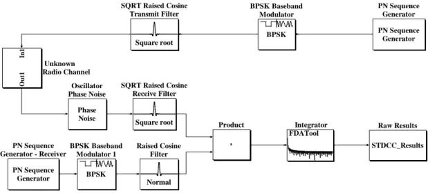
A. OFDM Sounder
Fig. 2 presents a baseband complex equivalent block diagram of the proposed OFDM sounder. For transmission, a pseudo-noise (PN) sequence of length M with an added zero is initially generated. Assuming BPSK (Binary Phase Shift Keying) modulation, the test sequence, with an equal number of zeroes and ones, is mapped into the test sequence with values of ±1. This sequence is transformed through an IDFT (Inverse Discrete Fourier Transform) using an IFFT (Inverse Fast Fourier Transform) algorithm of length M. Then, a square-root-raised-cosine transmission shaping filter is introduced, generating the transmitted analog signal. In the implementation employing Simulink®, the transmission shaping filter has an oversampling factor S, and from that, a signal sampled in discrete time is processed.
In the actual implementation of the receiver, the band pass analog signal is received, converted to baseband, filtered by a square-root-raised-cosine reception filter and sampled at twice the symbol rate, resulting in two samples per received symbol. This operation is performed in Simulink® by using a downsampling factor of in the square-root-raised-cosine reception filter.
Fig. 2. Baseband complex equivalent block diagram of the OFDM sounder
From there, the signal is split into two branches. In one branch, a symbol delay is introduced and the sequence of samples is downsampled by a factor of two. In the other branch, no delay is introduced, and the signal is subsampled by the same factor. Consequently, the first branch contains the even numbered samples of the signal, while the second contains the odd numbered samples. Next, a normalized DFT (Discrete Fourier Transform) is applied to the signals in each branch using a size M
FFT (Fast Fourier Transform) algorithm.
To estimate the response of the sounded channel in the frequency domain, the size M output of the FFT block (i.e., the received signal in the time domain with all the distortions introduced by the radio
2 Upsample1 2 Upsample In 1 O u t1 Unknown Radio Channel z 1 Unit Delay [A] Test Sequence1 [A] Test Sequence [A] Test Sequence
Sum Square root
SQRT Raised Cosine Transmit Filter Square root SQRT Raised Cosine Receive Filter Phase Noise Receiver Phase Noise OFDM_Results Raw Results Product1 Product PN Sequence Generator PN Sequence Generator Digital Filter Noise-Reduction Recursive Filter BPSK Mapping + or - 1
channel with their multipath) is divided, element by element, by the ±1 components of the test sequence. Two frequency domain channel representations are thus obtained – one for the odd numbered samples, and other for the even numbered samples.
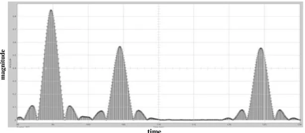
To obtain the channel impulse response estimate, the IDFT is applied once more to the odd and even sample results. After oversampled by a factor of two, the sequences are then added, with one shifted one position in time, to finally obtain an estimated channel impulse response with twice the number of samples. Fig. 3 shows the signals obtained in the time domain in the upper and lower branches, respectively and the final result for a simulated channel with three paths, wherein the delay of the second path is an integer multiple of the test symbol duration, Ts, and the delay of the third path is a non-integer multiple of this duration.
As the last processing stage to obtain raw data, a recursive low-pass filter can be inserted, with the objective of reducing the effects of the additive receiver noise (not considered here).
Finally, intermediate values are interpolated from those obtained by inserting a raised cosine low-pass filter, similar to the ones used in pulse shaping, with an oversampling factor S.
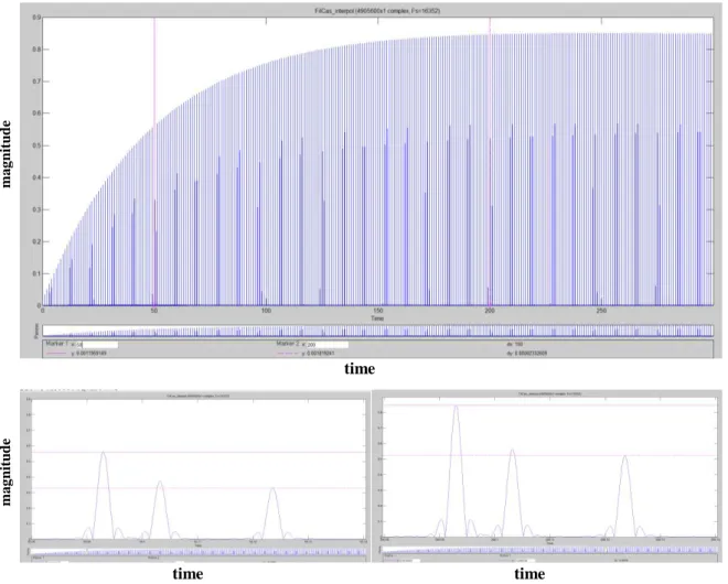
Fig. 3 (bottom) and 4 present the images of signals obtained through Simulink® before and after interpolation.
Fig. 4. Interpolator filter effect: OFDM generated estimates - magnitude
B. Matched Filter Sounder
Fig. 5 presents a baseband complex equivalent block diagram of the proposed Matched Filter sounder. In the Simulink® implementation, as in the OFDM section, the signal passes through the square-root-raised-cosine pulse shape reception filter and has two samples collected from each received symbol.
Fig. 5. Baseband complex equivalent block diagram of the Matched Filter sounder
In the matched filter implementation the coefficients of the filter matched to the test sequence are interleaved with zeroes, thus resulting in a FIR (Finite Impulse Response) filter of length 2 × N,
In 1 O u t1 Unknown Radio Channel u*Ts Sampler To=Ts/2 Square root SQRT Raised Cosine
Transmit Filter Square root SQRT Raised Cosine Receive Filter Phase Noise Receiver Phase Noise Matched_Filter_Results Raw Results Normal Raised Cosine Interpolation Filter PN Sequence Generator PN Sequence Generator Digital Filter Noise-Reduction Recursive Filter BPSK Mapping + or - 1
referred to as an interleaved matched filter. Fig. 6 represents the structure of this filter.
Fig. 6. FIR interleaved matched filter
Therefore, for every pulse of the clock, there is a shift in the sequence of samples of the received signal inside the interleaved matched filter, so that the samples are filtered, in turns, by the filter matched to the original test sequence; first the even numbered samples, and then the odd numbered ones. Thus here, as in the proposed OFDM sounder, the number of samples in the channel estimate is also doubled. It is important to emphasize that this zero interleaving procedure can be used for higher number of samples per symbol.
The processing of the signal at the output of the interleaved matched filter is identical to the one for the OFDM sounder. After the interpolation procedure, a file with the results is generated for future processing. Figures 3 (bottom) and 4 used in the description of the OFDM sounder are valid to represent the Matched Filter signal before and after interpolation. In Fig. 7, a single path channel estimate generated by the Matched Filter sounder is shown, with and without the use of the interleaved filter (one sample and two samples per symbol respectively), where the result obtained with the interleaved filter appears on the right side of the image.
Fig. 7. Estimated channel magnitude – Results obtained with one sample per symbol (left) and two samples per symbol (right)
Fig. 8 displays an image obtained with results generated by the Matched Filter sounder, showing
FIR interleaved filter output
0
±1
±1 0
FIR filter input
T0=Ts/2
odd, even, odd, even,
z-1
z-1
z-1
z-1
m
a
g
n
itu
d
e
the estimated channel modulus in one simulation. In the rising part of the envelope, the recursive filter convergence is noted. After convergence the sounder tracks the time variations of the channel magnitude. A new channel estimate is obtained for each test sequence received. The lower part of Fig. 8 shows a closer look at the channel estimates generated during and after convergence of the noise reduction IIR filter. An image similar to Fig. 8 was obtained with the OFDM method.
Fig. 8. Channel estimates generated by the Matched Filter sounder– Details during and after convergence of the IIR filter.
C. STDCC Sounder
Fig. 9 shows the equivalent baseband block diagram of the implemented wideband channel sounder using spectrum scattering, known as STDCC (swept time-delay cross-correlator). It should be noted that the STDCC is an analog traditional method used for radio channels estimations [3] [10].
In the STDCC method, the carrier is spread over a frequency band by a pseudo-noise (PN) test sequence signal of length M. This sequence has a bit period equal to and a bit rate equal to .
m
a
g
n
itu
d
e
m
a
g
n
itu
d
e
time
Fig. 9. Baseband complex equivalent block diagram of the STDCC sounder
In this method, the received scattered signal is correlated with an identical PN sequence signal generated in the receiver. Although the two sequences have identical content, the clock that determines the bit rate of the transmitter has a slightly higher frequency than the receiver. A sliding correlator is implemented mixing and filtering the two sequences. When the higher rate transmitted PN sequence aligns with the lower rate receiver generated sequence, a correlation peak occurs.
The STDCC method has an equivalent time measurement, which is updated every time the two sequences are correlated to the fullest. The elapsed time between two adjacent maximum correlations is calculated by:
(4)
where:
: bit period (s);
: bit clock frequency (Hz); : slide factor (dimensionless);
: PN sequence length (bit)
The slide factor is defined as the relationship between the rate of transmission bit clock and the difference between clock rates of transmission and reception. Mathematically is expressed as:
(5)
where,
: transmitter bit clock rate (Hz); : receiver bit clock rate (Hz).
It should be noticed that in the time period required by the STDCC method to generate one single channel estimate result, the other two methods produces channel estimates.
Square root SQRT Raised Cosine
Transmit Filter
Square root SQRT Raised Cosine
Receive Filter
STDCC_Results Raw Results
Normal Raised Cosine
Filter
Product
PN Sequence Generator PN Sequence Generator - Receiver
PN Sequence Generator PN Sequence
Generator
Phase Noise Oscillator Phase Noise
BPSK BPSK Baseband
Modulator 1
BPSK BPSK Baseband
Modulator
In
1
O
u
t1
Unknown Radio Channel
IV. PRIMARY CALCULATED PARAMETERS
The simulation was conducted for an ensemble of ten sample functions of phase noise for each of nine different values of the ratio carrier power to the power spectral density of phase noise at a given off-set frequency. Final results are an average over the considered ensemble.
The simulated channel used as a reference is selective both in time and in frequency. The selectivity in time is associated with the Doppler spread while the selectivity in frequency is associated with time scattering arising from resolved multipath. The simulation considered an N-path channel. The amplitudes of the paths were modeled as independent complex wide-sense stationary, Gaussian processes with power spectral densities given by the Jakes model [11]. This model has the Doppler frequency as a parameter and is frequently used in mobile communication scenarios. The description of the simulated channel model used by Matlab® is presented in [9].
After obtaining the channel estimation results, the three methods were compared computing the ratio between the estimated channel ratio and the reference channel ratio according to.
= (6)
where 2≤ n ≤ N , and n > k.
In (6), N denotes the total number of existing paths in the search environment, and n and k represent the arriving order of the path at the sounder mobile receiver. Since the coefficients of the estimated channel and the reference channel, are, in general, complex the ratio defined in (6) has modulus, , and phase . An ideal estimation would result in and .
For the simulated radio channel to be considered approximately time invariant the value of product was assumed equal to 10-4, where represents the maximum Doppler shift and T is the test sequence period.
V. NUMERICAL RESULTS
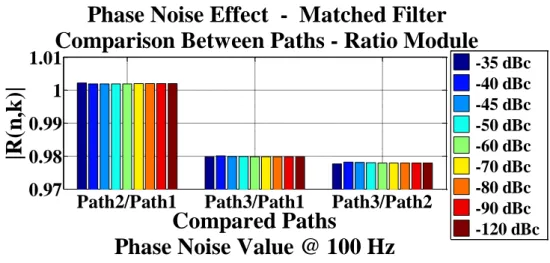
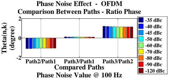
Fig. 10 presents modulus and phase results obtained from (6) for each simulated phase noise value.
a) Matched Filter
Path2/Path1
Path3/Path1
Path3/Path2
0.97
0.98
0.99
1
1.01
Compared Paths
Phase Noise Value @ 100 Hz
|R
(n
,k)
|
Phase Noise Effect - Matched Filter
Comparison Between Paths - Ratio Module
b) OFDM
(c) STDCC
Fig. 10. Results after use of (6) for the three methods
From the results shown in Fig. 10 both the precision and the dispersion were analyzed for each method according to the calculated parameters.
Path2/Path1
Path3/Path1
Path3/Path2
-2
0
2
Compared Paths
Phase Noise Value @ 100 Hz
T
het
a
(n,k)
(de
g
re
e)
Phase Noise Effect - OFDM
Comparison Between Paths - Ratio Phase
RMS value of the ratio error, ;
Standard deviation of the ratio modulus, ;
RMS value of the complex ratio phase, ;
Standard deviation of the ratio, phase, .
The RMS error and standard deviation results were computed over nine different simulated values of phase noise.
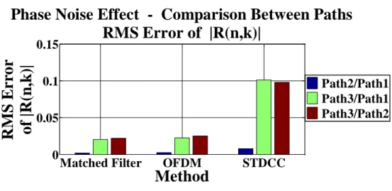
Fig. 11 shows the ratio RMS error. Notice a similar performance between Matched Filter and OFDM methods. Both have a very precise result considering the path2/path1 ratio and less than 2.5% error when path3 is computed. Also the STDCC method presents a better performance when estimating the path2/path1 ratio, however four times worse than Matched Filter method (0.008/0.002). Again the STDCC method is worse than the others when path 3 is considered, showing an estimated RMS error of about 10%.
Fig. 11. RMS error of
Fig. 12 shows the Matched Filter as the method with lower sensibility to variations in the phase noise levels closely followed by the OFDM method. But, interestingly, in STDCC method the path2/path1 ratio is more susceptible to the presence of phase noise. Fig. 10 (c) shows that between -35 dBc and -60 dBc the phase noise changes the STDCC results considerably but only a small effect is observed for lower dBc values.
Matched Filter OFDM STDCC
0 0.05 0.1 0.15
Method
R
M
S
E
rr
o
r
o
f
|R
(n
,k
)|
Phase Noise Effect - Comparison Between Paths
RMS Error of |R(n,k)|
Fig. 12. Standard deviation of
The RMS values of presented in Fig. 13 indicate that variations in the phase noise levels have small impact on precision of the methods. The maximum detected value is approximately 1.3º.
Fig. 13. RMS error of
Still considering the ratio phase error, , from the point of view of sensitivity to phase noise level variation indicated by the standard deviation values of Fig. 14, the STDCC method is the worse, when compared with the other two methods. However, the standard deviation values are all very small with estimated value of about 0.4º.
Matched Filter OFDM STDCC
0 2 4 6 8x 10
-3
Method
St
a
nd
a
rd
D
ev
ia
ti
o
n
o
f
|R
(n,k
)|
Phase Noise Effect - Comparison Between Paths
Standard Deviation of |R(n,k)|
Path2/Path1 Path3/Path1 Path3/Path2
Matched Filter OFDM STDCC
0 0.5 1 1.5
Method
R
M
S
E
rr
o
r
o
f
T
het
a
(n
,
k
)
(d
eg
re
e)
Phase Noise Effect - Comparison Between Paths
RMS Error of Ratio Phase
Path2/Path1 Path3/Path1
Fig. 14. Standard deviation of
VI. CONCLUSION
In this work three wideband mobile radio channel sounding methods were simulated using computational tools. The implemented sounders included the traditional STDCC and two other proposed sounding methods, based on OFDM digital transmission and detection procedures and on matched filtering. The impact of the phase noise introduced by the local oscillator in the precision of the examined sounders was analyzed by comparing the simulated reference channel with the estimated channel results for several different phase noise levels. Other impairments factors like thermal noise or nonlinear distortion affecting the system were not considered. The OFDM and Matched Filter methods collect and process more samples per received symbol aiming at increasing precision of the estimation method before interpolation
Considering the ratio error, , the Matched Filter and OFDM methods presented RMS values smaller than 2.5%, while the STDCC results reached 10% for the path3/path1 ratio. The results for the standard deviation of indicated the STDCC method as the most sensitive to phase noise levels variations, even though the higher estimated value, 0.8%, is not relevant in field measurements. Concerning the values of the ratio phase, , the STDCC method was also the less reliable, although the RMS error and standard deviation results presented negligible values for all compared methods.
An analysis of the results shown in Fig. 10, indicate that phase noise levels lower than -60 dBc @ 100 Hz off-set frequency have no significant impact on the precision of the analyzed methods.
Finally, apart from oscillator phase noise effects, it should be emphasized, as mentioned in the previous section, that during the time period required by the traditional STDCC method to generate a single channel estimate the other sounding methods are able to generate several channel estimates snapshots. This advantage is particularly important for the sounding and statistical characterization of time varying channels.
Matched Filter
OFDM
STDCC
0
0.1
0.2
0.3
0.4
Method
St
a
nd
a
rd
D
ev
ia
ti
o
n
o
f
T
het
a
(n
,
k
)
(d
eg
re
e)
Phase Noise Effect - Comparison Between Paths
Standard Deviation of Ratio Phase
REFERENCES
[1] B. Sklar, “Rayleigh fading channels in mobile digital communication systems, Part II: Mitigation”, IEEE
Communications magazine, pp. 102-109, July, 1997.
[2] C. E. S. Ferreira, “Comparison among wideband mobile radio channel sounding techniques in the presence of sounder
imperfections”, Doctoral thesis, Electrical Engineering Department, Pontifical Catholic University of Rio de Janeiro, 2013.
[3] J.D. Parsons, D.A. Demery, A.M.D. Turkmani, “Sounding techniques for wideband mobile radio channels: a review”,
IEE Proceedings-1, Vol. 138, No.5, October 1991.
[4] D. B. Leeson, “A simple model of feedback oscillator noise spectrum”, Proceedings of the IEEE, volume 54, issue 2, pg
329-330, 1966.
[5] G. Sauvage, “Phase noise in oscillators: A mathematical analysis of Leeson’s model”, IEEE Transactions on
Instrumentation and Measurements, vol. IM-26, NO. 4, 1977.
[6] X. Huang, F. Tan, W. Wei, and W. Fu, “A revisit to phase noise model of Leeson”, Frequency control Symposium,
2007 joint with the 21st European Frequency and Time Forum, IEEE International, pg. 238-241, 2007.
[7] N. J. Kasdin,”Discrete simulation of colored noise and stochastic processes and 1/fα power law noise generator”,
Proceedings of the IEEE, , Volume: 83, Issue: 5, Page(s): 802 – 827, May 1995.
[8] A. G. Armada, “Understanding the effects of phase noise in orthogonal frequency division multiplexing (OFDM)”,
IEEE Transactions on Broadcasting, Volume: 47, Issue: 2, Page(s): 153 – 159, Jun 2001.
[9] C. D. Isklander, “A MATLAB®-based object-oriented approach to multipath fading channel simulation”, Hi-Tek
Multisystems, Québec, Canada, http://www.mathworks.com/matlabcentral/fileexchange/18869-a-matlab-based-object-oriented-approach-to-multipath-fading-channel-simulation, 21 Feb 2008.
[10] Ryan J. Pirkl, Gregory D. Durgin, “Optimal sliding correlator channel sounder design”, IEEE Transactions on Wireless
Communications, Vol. 7, NO. 9, September 2008
[11] M. J Gans, “A power-spectral theory of propagation in the mobile-radio environmen”, IEEE Transactions on Vehicular
Technology;Vol. 21, Iss. 1, pp. 27-38, 1972.
[12] B. Muquet, Z. Wang, G. B. Giannakis, M. de Courville, P. Duhamel, “Cyclic Prefixing or Zero Padding for Wireless
APPENDIX
Wideband sounding
Wideband radio channel characterization comprises both the quantity of multipath components present in a particular environment and the way in which they affect the reception, each with their own delay, amplitude and phase. This information creates a time-delay profile.
The sounding of the wideband radio channel is thus an essential tool for systems development and there are different ways to implement it. Alternatives for the construction of wideband sounders are presented, aiming at the increase in the precision of the estimated parameters.
1. Theoretical Basis of Pulse Compression
The analysis of pulse compression systems is based on linear systems theory. It is known that if a white noise signal is applied to the input of a linear time-invariant system and the output is correlated with a delayed input replica , the resulting cross-correlation will be proportional to the impulse response of the system, evaluated in the time delay . The white noise autocorrelation function is given by
(A.1) where denotes the expected value operator or expectation, (.)* represents the complex conjugate, is the autocorrelation function of the process , is the single-sideband noise power spectral density, and is the Dirac delta function In time domain, a continuous output signal is obtained through the convolution integral
(A.2)
Thus, the cross-correlation between the output and delayed input is given by:
(A.3)
Therefore, the impulse response of a linear system can be estimated by using a source of white noise and a method to process the correlation between the output signal and the delayed input test signal.
In practice, the systems that apply pulse compression use deterministic waveforms with autocorrelation characteristics similar to the white noise autocorrelation. An easily generated and widely used sequence is the maximum length pseudorandom binary sequence, also known as the pseudo-noise sequence (PN sequence).
1.1. Matched Filters
represents the quantities in the frequency domain, as opposed to quantities in the time domain, such as the coefficients of the channel impulse response or the samples that are effectively carried through waveforms transmitted in the propagation channel. The symbol ⊗denotes circular convolution and the symbol denotes linear convolution.
The matched filter sounding method should be considered as a digital method. A known sequence of test that has autocorrelation similar to that of white noise is used. For the remainder of this appendix, the PN sequence is adopted as the test signal to be transmitted. A finite impulse response FIR filter whose impulse response corresponds to the transmitted PN sequence reversed in time, i.e., a filter matched to the test signal, is used in the receiver.
The periodic test sequence represented by , whose period has length and duration ,
were represents the duration of each symbol can be identified as the output of a Binary Phase Shift Keying BPSK modulator whose input is a pseudorandom binary sequence of length N, the elements of which are zeroes and ones obeying their laws of formation. Assuming the amplitude of the BPSK symbols to be equal to , a single period of the periodic test sequence can be represented by the block:
(A.4) For the spectrum shaping of the signal to be transmitted, the classical theory represents a linear modulated channel in baseband. An ideal transmission system is displayed in Fig. A.1, in which necessary changes were introduced to represent the sounding method named “Matched Filter.”
Fig. A.1 – Block diagram of matched filter sounders
In Fig. A.1, the block identified by represents the transmission square-root-raised-cosine pulse shape filter, the block represents the propagation channel impulse response, the block represents the receiver filter, which is matched to the transmission filter, and is the white noise present at the input of the receiver. Following these blocks, a sampler operating at symbol rate takes samples of the analog output of the receiver filter. Finally, the Matched Filter is inserted, which is matched to the test sequence and is indicated by block .
Let be the analog system impulse response, given by the convolution of the shaping transmission filter with the channel impulse response and with the receiver filter, them the discrete time system impulse response is given by:
(A.5)
In the absence of noise in the input of the receiver, the output of the filter matched to the test sequence is represented by:
(A.6)
Considering that the radio channel varies slowly enough to not change significantly during the transmission of a PN sequence, and since the test sequence is periodic, the convolution indicated in (A.6) can be considered to be circular. Denoting by the segment of resulting from the i-th repetition of the test sequence a, we have:
⊗ , (A.7)
In addition, considering that ⊗ is the circular autocorrelation of the PN sequence, and knowing that:
then can be represented as:
(A.8) where is the discrete time impulse defined by:
Therefore from (A.7) and (A.8) it results
(A.9)
where is the value of the discrete system frequency response at zero frequency resulting from
(A.10)
where and L represents the length of the response of the system to a discrete impulse. From (A.9), we have that:
(A.11)
and assuming that the PN sequence is sufficiently long:
(A.12)
Finally, we observe that:
N must be greater than the span of to avoid superposition ( )
Regarding the resolution the time interval between the paths of must be greater than the span of .
2 OFDM
2.1 Notations
Matrix WM implements the Discrete Fourier Transform (DFT) of size M, whose elements are
. The ⊙ symbol represents the product of two vectors, term by term, and (.)H
indicates the Hermitian transposition.
2.2 OFDM sounder
The idea behind the OFDM transmission technique using the so called cyclic prefix is to make the linear convolution of the transmitted signal with the channel impulse response equivalent to a circular convolution. The resulting circular convolution is then transformed into a multiplication in the frequency domain. The principle behind this operation is shown in Fig. A.2. In this figure, the difference between circular and linear convolution is illustrated for the case of the repeated transmission of blocks of symbols, . The circular convolution of the periodic sequence of blocks with the channel impulse response h that results in r(i) is displayed in Fig. A.2(a). In the frequency domain, we than have:
(A.13)
It becomes clear from the superimposition in the beginning of the block that the result of the linear convolution of [..., s(i-1), s(i), s(i+1), ...]with h is, in general, not equal to the circular convolution. In fact, there is no reason for the end of the block to be equal to the end of the s(i) block. In addition, the output of the channel corresponding to the block is superimposed onto the output of the previous block , the so called interblock interference. The cyclic prefix principle introduces redundancy in the transmitted signal in such a way that the superimposition induced by the channel memory corresponds to that of the circular convolution. In this way, the block of symbols that correspond to the transmission of s(i) is exactly the same as the circular convolution of s(i) and h. Therefore, s(i) is easily recovered from the received r(i) block by performing a DFT. Furthermore, r(i) becomes independent from the s(i-1) block, which is important since the recovery of
Fig. A.2 – Cyclic prefix principle
The implemented OFDM system used as a sounding method of the radio mobile channel is based on the OFDM principle, whose transceiver scheme is described in Fig. A.3. This figure represents the baseband equivalent in the discrete time domain. In theory, it is assumed that both the transmitted and received signals are sampled in synchrony with the system basic rate, and the focus will be on OFDM discrete time aspects.
In the baseband equivalent model of the OFDM sounder transceiver, the complex symbols representing the points of the signal constellation of the adopted modulation are transmitted in blocks of length M: that forms the test sequence. These symbols are initially transformed by the IDFT unity matrix , whose elements are , which transforms the block to the time domain now denoted by block. The channel is represented by its equivalent discrete time domain model, and its effect is modeled as a time variant linear filter with a size L finite impulse response FIR, represented by the impulse response
r(i)=h⊗s(i)
s(i) s(i) s(i)
h
a – Circular
Channel impulse response
DFT(r(i))=DFT(h)×DFT(s(i))
Result of circular convolution
s(i-1) s(i) s(i+1)
h
b – Linear Convolution
Channel impulse response
Does not correspond to a circular convolution
Corresponds to
circular convolution Superimposes on
block s(i+1)
s(i) s(i+1)
h
c – Cyclic prefix insertion
Channel impulse response
Corresponds to circular convolution:
DFT(r)=DFT(h)×DFT(s(i)
)
s(i-1)
where L-1 is the channel order. It is assumed here that the channel does not change that during the test sequence transmission time. This is a fair approximation if the product where is the maximum Doppler shift and is the test sequence duration. Since the test sequence length is made bigger than the channel order, , the mobile radio channel can be estimated without ambiguity. The length M impulse response is defined as appended with zeroes until the length M is reached.
Fig. A.3 – Discrete model for an OFDM conventional transceiver
The size M test sequence is IDFT transformed by the matrix . In time domain the transmitted block of symbols is then . The received block of symbols corresponds to the circular convolution between and plus the noise contribution where represents a vector of complex noise samples in the receiver’s baseband equivalent
model of the sounder. Hence, the received time domain vector can be expressed by:
⊗ (A.14)
The circular convolution presented in equation (A.14) may be expressed in matrix form:
(A.15)
The elements of each matrix column are obtained shifting the elements of the previous column circularly by one position. Since this matrix is a circulant matrix it can be diagonalized by
Discrete time equivalent
channel
Parallel to serial converter
Modulator Serial to
parallel converter
Demodulator
pre- and post-multiplication by unitary DFT and IDFT matrices. Therefore,
(A.16)
In (A.16), represents a M×M diagonal matrix whose elements are the components of the vector transformed to the frequency domain whereas
is the noise vector at the receiver imput transformed to the frequency domain. The equation (A.16) can be rewritten as:
⊙ (A.17)
It then results that the n-th component of , denoted by , can be independently detected from the others without intersymbol interference between adjacent test sequence symbols. Expression (A.17) can be rewritten as:
(A.18)
where and are the nth components of the channel frequency response and the noise vector , respectively. Since the test sequence is known, the estimation of the channel frequency response at the receiver is obtained by dividing each element of the received signal by each element of the test signal. Observing that is an M×M diagonal matrix that contains the reciprocal of each element and the channel is considered time invariant during each test sequence transmission, an estimate of the channel impulse response is given by:
(A.19)
It is clear that the noise present at the receiver will affect the accuracy of the channel estimation. Finally, the estimated impulse response of the sounded channel is given by: