ISSN 0104-6632 Printed in Brazil
www.abeq.org.br/bjche
Vol. 31, No. 04, pp. 977 - 991, October - December, 2014 dx.doi.org/10.1590/0104-6632.20140314s00003084
Brazilian Journal
of Chemical
Engineering
COMPARISON OF AN IMPEC AND A
SEMI-IMPLICIT FORMULATION FOR COMPOSITIONAL
RESERVOIR SIMULATION
B. R. B. Fernandes
1, A. Varavei
2, F. Marcondes
3*and K. Sepehrnoori
41Laboratory of Computational Fluid Dynamics, Federal University of Ceará, Brazil. 2
Center for Petroleum and Geosystems Engineering, The University of Texas at Austin, USA.
3
Department of Metallurgy and Materials Science and Engineering, Federal University of Ceará, Brazil. E-mail: [email protected]
4
Center for Petroleum and Geosystems Engineering, The University of Texas at Austin, USA.
(Submitted: November 1, 2013 ; Revised: January 16, 2014 ; Accepted: February 21, 2014)
Abstract - In compositional reservoir simulation, a set of non-linear partial differential equations must be solved. In this work, two numerical formulations are compared. The first formulation is based on an implicit pressure and explicit composition (IMPEC) procedure, and the second formulation uses an implicit pressure and implicit saturation (IMPSAT). The main goal of this work is to compare the formulations in terms of computational times for solving 2D and 3D compositional reservoir simulation case studies. In the comparison, both UDS (Upwind difference scheme) and third order TVD schemes were used. The computational results for the aforementioned formulations and the two interpolation functions are presented for several case studies involving homogeneous and heterogeneous reservoirs. Based on our comparison of IMPEC and IMPSAT formulations using several case studies presented in this work, the IMPSAT formulation was faster than the IMPEC formulation.
Keywords: Compositional reservoir simulation; Segregated formulation; IMPEC; IMPSAT; Finite-volume method.
INTRODUCTION
Several formulations have been developed for solving the governing partial differential equations arising from modeling fluid flow for compositional simulations in porous media. In general, formula-tions can be classified as Implicit Pressure Explicit Composition (IMPEC), Implicit Pressure and Satura-tion (IMPSAT), or the Fully Implicit Method (FIM). Phase saturation is defined as a volume of phase per void space available for fluid flow. The IMPEC for-mulation has the lowest cost in terms of computa-tional time per time-step. However, due to the higher degree of explicitness in the calculation of composi-tion, this formulation cannot use large time-steps when compared to the FIM and IMPSAT approaches.
The IMPSAT method can handle larger time-steps, compared to the IMPEC approach. It is also less expensive in terms of computational time, per time-step, than the FIM approach. Additionally, the IMPSAT approach is more stable than the IMPEC formulation due to the reduction in the degree of explicitness. Also, according to Cao (2002), it has good performance compared to other FIM approaches, since saturations are much more coupled than com-positions. Therefore, although the saturation calcula-tion involves solucalcula-tion of a linear system of equacalcula-tions for the IMPSAT formulation, the larger time-steps used by the formulation compensate the overall cost and render a CPU time reduction compared to IMPEC approaches.
Brazilian Journal of Chemical Engineering
Watts (1986) was implemented into the UTCOMP simulator. UTCOMP was developed at the Center for Petroleum and Geosystems Engineering at The University of Texas at Austin for the simulation of enhanced recovery processes. The UTCOMP simula-tor is a multiphase/multi-component compositional equation-of-state simulator, which can handle the simulation of several enhanced oil recovery processes. The original numerical procedure of the UTCOMP simulator is an IMPEC formulation based on Àcs et al. (1985).
Several procedures for solving pressure and satu-ration implicitly (IMPSAT) have been proposed in the literature (Branco and Rodrigues, 1996; Kendall et al., 1983; Spillette et al., 1973). However, the IMPSAT approach proposed by Watts (1986) and adopted in this work has similar features to the original IMPEC formulation of the UTCOMP simulator. For instance, the IMPSAT formulation solves simple sets of linear systems for both pressure and saturations, while only one flash procedure is performed per time-step, thus allowing the calculations per time-step to be much faster than the other IMPSAT and IMPEC approaches that need iterations, thus performing flash and solving the conservation equations until convergence. The approaches that do not iterate in a time level are called one-iteration formulations; therefore, this work is based on a comparison of two one-iteration ap-proaches: an IMPEC and an IMPSAT formulation. Although the IMPEC and IMPSAT formulations im-plemented and used in this work are not new, to the best of our knowledge this is the first time that these formulations are compared for three phase hydrocar-bon flow simulations (oil, gas, and a second liquid hydrocarbon phase). The second liquid hydrocarbon phase is important for CO2 injection processes, where
the CO2 and some light components tend to form a
CO2-rich phase. Another important feature included in
this work is the use of a high-resolution TVD scheme to approximate the fluxes for the Watts’ formulation. Also, only few performance results are shown in the literature for this formulation. Some of these results can be found in Haukås (2006). In this work, results are compared in terms of volumetric production rates, saturation fields, and CPU time. For most investigated cases, the formulation was able to use larger time-steps than the IMPEC formulation, achieving the same results.
PHYSICAL MODEL
The Watts’ formulation is basically an adaptation of the method of Spillette et al. (1973) combined
with the formulation of Ács et al. (1985), where the volume error constraint is added to pressure and satu-ration equations in order to use just only one flash calculation per time-step. In this section, we show the molar balance equations, the pressure equation, and the new saturation equations that are included in the original formulation of Ács et al. (1985).
If advection is the only transport mechanism in-volved, the molar balance equations according to Chang (1990) are given by
1 1
,
1, ..., , 1
p
N
r j
k k
kj j j
b j j b
c c
k
N q
x K
V t V
k N N
=
⎛ ⎞
∂ = ∇ ⋅ ξ ⋅∇Φ −
⎜ ⎟
⎜ ⎟
∂ ⎝ μ ⎠
= +
∑
G G, (1)
where Nk is the moles of component k, Vb is the bulk
volume, xkj is the mole fraction of component k in
phase j, ξj is the molar density, respectively, qk is the
molar rate of component k through the well, Nc is the
number of hydrocarbon components, Nc+1 denotes
the water component, krj and µj are the relative
per-meability and viscosity of phase j, respectively, K is the absolute permeability tensor, and Φj is the
hy-draulic potential of phase j, which is defined by
,
j P jgD Pcjr
Φ = − ρ − (2)
where P is the pressure of the oil phase, ρj is the
mass density of phase j, g is the gravity, D is the depth, which is positive in the downward direction, and Pcrj is the capillary pressure between phases j
and r.
Fluid phase equilibrium between the hydrocarbon phases is considered (water is not considered in any flash calculation). This assumption considers that the chemical potential of all phases are the same. This can be expressed in terms of the equality of the fuga-cities (f) of the phases, which can be stated as follows:
0, 1, ..., .
o g
i i c
f −f = i= N (3)
volume-shift approach based on the work of Jhaveri and Youngren (1988) is also available for liquid density correction.
Two phase stability test algorithms are imple-mented in the UTCOMP simulator: the stationary point location method (Michelsen, 1982) and the Gibbs free energy minimization algorithm, which is similar to the Trangenstein (1987) method and was modified by Perschke (1988) to deal with three hy-drocarbon phase equilibrium. In general, as com-mented by Perschke (1988), the stationary method is faster than the Gibbs free energy method; therefore, the stationary method was used in this work. The flash calculation used in UTCOMP is a combination of the Accelerated Successive Substitution (ACSS) method (Mehra et al., 1983) with the modified ver-sion of the Gibbs free energy minimization method (Perschke, 1988). At the beginning of the flash pro-cedure, we use the ACSS method in order to provide a reasonable initial estimation, and then we switch to the Gibbs free energy minimization method in order to accelerate the convergence. The switching crite-rion to change from one method to another is given by Chang (1990) as:
2
max ln ln
for 1,..., 3,..., ,
− ≤ ε
= = j i swi i c p f f
i N and j N
(4)
where, the superscript 2 denotes the oil phase. The switching criterion (εswi) equal to 0.01 as suggested
by Chang (1990) is used.
The pressure equation used for both formulations is based on the volume constraint proposed by Ács et al. (1985). The pressure equation is obtained from the equality between the formation pore volume (Vp)
and the total fluid volume (Vt):
1 1
( ) ( , ,..., , ),
c c
p t N N
V P =V P N N N + (5)
where the pore volume is given by:
(
)
0 1 ,
p b f f
V = φV ⎡⎣ +c P−P ⎤⎦ (6)
where φo is the porosity at the reference pressure
(Pf), and cf is the rock compressibility.
Taking the derivative of Eq. (5) with respect to time, applying the chain rule to the right-hand side, substituting Eqs. (1) and (6), and dividing all by the bulk volume, we obtain
0 1 , ( ) 1 1 1 , p c s t f b N N N r j t k
kj j j
k P N s i j b
k j
P V P
c
t V P t
k V q x K N V + ≠ = = ∂ ⎛∂ ⎞ ∂
φ = ⎜ ⎟
∂ ⎝∂ ⎠ ∂
⎡ ⎛ ⎞ ⎤
⎛∂ ⎞ ⎢ ⎥
+ ⎜∂ ⎟ ⎢ ∇⋅⎜⎜ ξ μ ⋅∇Φ +⎟⎟ ⎥
⎝ ⎠ ⎣ ⎝ ⎠ ⎦
∑
∑
G G(7)
where N denotes derivative evaluated by holding the number of moles constant.
The saturation equation is solved implicitly only for the IMPSAT formulation. The approach used here is described by Watts (1986). By definition, the saturation of phase ℓ (Sℓ), as stated before, is the ratio of the phase volume to the volume of the pore:
, p V S V = A
A (8)
where Vℓ is the volume of phase ℓ, which is a
func-tion of pressure and number of moles. Equafunc-tion (8) can be written as:
1 1
( ) ( , ,..., , ).
c c
p N N
S VA P =V P NA N N + (9)
Taking the derivative of Eq. (9) with respect to time, applying the chain rule on the right-hand side and substituting Eq. (1) and dividing it by the bulk volume, we obtain:
(
)
(
)
1 , ( ) 1 1 1 1 . p c s pb b N
N N
k kj j j
k P N s i b
k j
V P
S V
V t V P t
V q x v N V + ≠ = = ∂ = ⎛∂ ⎞ ∂ ⎜ ⎟ ∂ ⎝ ∂ ⎠ ∂ ⎛ ⎞ ⎛∂ ⎞ ⎜ ⎟
+ ⎜ ⎟ ∇ ⋅ ξ +
∂ ⎜ ⎟
⎝ ⎠ ⎝ ⎠
∑
∑
A A
A G G
(10)
Brazilian Journal of Chemical Engineering
(
)
(
)
1
,
Np
j m
j j t m
cjo cmo m
g D
v f v K
P P
=
⎡ ⎛ ρ − ρ ∇ ⎞⎤
= ⎢ + λ ⋅⎜⎜ ⎟⎟⎥
+∇ −
⎢ ⎝ ⎠⎥
⎣
∑
⎦G
G G G
(11)
where
rm m
m
k
λ =
μ , (12)
1 1
( )
Np Np
t i j cjo j
i j
v v K P P g D
= =
=
∑
= −∑
λ ⋅ ∇ + ∇G G − ρ ∇GG G , (13)
and,
1 ,
j j Np
m m
f
= λ =
λ
∑
(14)where, vGt is the total fluid velocity, λm is the m-th
phase mobility which is defined as a ratio of relative permeability and viscosity of the m-th phase, and fj is
called the fractional flow, which is defined as above. Substituting Eq. (11) into (10) yields:
(
)
(
)
(
)
(
)
1
, ( )
1 1
, ( )
1 1 1
1 1
.
c
s p
c
s
N
k p
b b N k k P N s i b
N
N Np
kj j j t m j m cjo cmo
k P N s i
k j m
V P V q
S V
V t V P t N V
V
x f v K g D P P
N
+
≠ =
+
≠
= = =
⎛ ⎞ ⎛ ⎞
∂ = ⎛∂ ⎞ ∂ + ∂ +
⎜ ⎟ ⎜ ⎟
⎜ ⎟
∂ ⎝ ∂ ⎠ ∂ ⎝∂ ⎠ ⎝ ⎠
⎛ ⎡ ⎛ ⎞⎤⎞
⎛∂ ⎞ ⎜ ∇ ⋅⎢ ξ ⎜ + λ ⋅ ρ − ρ ∇ + ∇ − ⎟⎥⎟
⎜∂ ⎟ ⎜ ⎜ ⎟ ⎟
⎢ ⎥
⎝ ⎠ ⎝ ⎣ ⎝ ⎠⎦⎠
∑
∑
∑
∑
A A
A
A G G G G
(15)
Equation (15) is the final saturation equation in terms of total velocity. The next section is devoted to showing the numerical discretization applied to the above equation.
APPROXIMATE EQUATIONS
In order to obtain an approximate equation for the saturation of phase ℓ, we will integrate Eq. (15) over the control volume of Figure 1 and time.
Figure 1: Control volume.
,
, ,
, ,
, ,
1 1 1
, , , , , , 1 1 1 1 1 1
1 1 1
( ) + + + + + = + + + = = = ⎛ ⎞ ⎛∂ ⎞ ⎜ ⎟ − −⎜⎜ ⎟⎟ − + −
∂ ⎜ ξ ⎟
⎝ ⎠ ⎝ ⎠
= Δ
⎧ ⎫ ⎧
⎪ ⎡ ⎤⎪ ⎪ ⎡ ⎤
+Δ ⎨ ⎢ ξ ⎥⎬− Δ ⎨ ⎢ ξ ⎥
⎣ ⎦ ⎣ ⎦ ⎪ ⎪ ⎪ ⎩ ⎭ ⎩
∑
∑
∑
∑
A A A A A AA A A
P c
k P k P
p p
c
k P kj j k P kj j
n n
P P
n n n n n n n n
P p P P p P P P P p P n
P N N n n k N N N
n n n n n n n n
j j
e w
k j j
V n
S V S V P P S V
P
t V q
t V x u t V x u
, , , , 1 1 1 1 1 1
1 1 1 1
1 1 1 1 1 , + = + + + + = = = = + + + = = = ⎫⎪ ⎬ ⎪⎭ ⎧ ⎫ ⎧ ⎫ ⎪ ⎡ ⎤⎪ ⎪ ⎡ ⎤⎪
+Δ ⎨ ⎢ ξ ⎥⎬− Δ ⎨ ⎢ ξ ⎥⎬
⎣ ⎦ ⎣ ⎦
⎪ ⎪ ⎪ ⎪
⎩ ⎭ ⎩ ⎭
⎧ ⎫
⎪ ⎡ ⎤⎪ ⎡ ⎤
+Δ ⎨ ⎢ ξ ⎥⎬− Δ ⎢ ξ ⎥
⎣ ⎦ ⎣ ⎦ ⎪ ⎪ ⎩ ⎭
∑
∑
∑
∑
∑
∑
∑
A A A A c p p c ck P kj j k P kj j
p c
k P kj j k P kj j
N
k
N N
N N
n n n n n n n n
j j
n s
k j k j
N N
n n n n n n n n
j j
f b
k j j
t V x v t V x v
t V x w t V x w
1 1 1 + = ⎧ ⎫ ⎪ ⎪ ⎨ ⎬ ⎪ ⎪ ⎩ ⎭
∑
c∑
NpN
k
(16)
where tk
V is the total volume derivative with respect to total number of moles of component k, and nj 1
e
u + is a semi-implicit velocity at the east interface, which is given by:
{
(
)
(
)
(
) (
)
}
1
1 1 1
1 1
1
1 1 1 1
, , , ,
,
p
n Np
j
n e n n n n
j N t xe m j E P m E P
e e e e e
m n
m e m
n n n n
cmo E cmo P cjo E cjo P
u u T g D D g D D
P P P P
+ + + + = + = + + + + λ ⎡
= + λ ⎢⎣ ρ − − ρ −
λ ⎤ + − − − ⎦
∑
∑
(17) where, 2 . x ex P x E
y z T x x K K Δ Δ =
Δ +Δ (18)
The semi-implicit velocity, at the other interfaces, is given by equations similar to Eq. (17). Newton’s method is used to treat the non-linearities involved in Eqs. (16) and (17) on account of the implicit evaluation of the relative permeabilities and capillary pressures.
Performing a similar procedure for the saturation equation, we obtain the approximate mole balance equations, in terms of the semi-implicit velocity, as given below:
( )
( )
( )
( )
( )
( )
,
1
, , 1 1 1
1 1
1 1 1 1
1 1 1 1
+
-+ - + - .
p p
k P kj j kj j
p p p p
kj j kj j kj j kj j
N N
n n
k P k P n n n n n n n
j j
e w
e w
j j
N N N N
n n n n n n n n n n n n
j j j j
n s f b
n s f b
j j j j
N N
q x u x u
t
x v x v x w x w
+ + + + = = + + + + = = = = ⎛ − ⎞ ⎡ ⎤ ⎡ ⎤
= ξ ξ
⎜ ⎟ ⎢ ⎥ ⎢ ⎥
⎜ Δ ⎟ ⎣ ⎦ ⎣ ⎦
⎝ ⎠
⎡ ⎤
⎡ ξ ⎤ ⎡ ξ ⎤ ξ ⎡ ξ ⎤
Brazilian Journal of Chemical Engineering
The final form of the pressure equation is obtained (considering only the x direction for simplicity) as:
(
)
(
)
(
)
, , , , , 1 , ,0 1 1
, , 1 1 1 1 1 1 1 1 , 1 ( ) + + + = = + + + = = + = ⎛ ⎞ ⎛ ⎛∂ ⎞ ⎞ ⎜ ⎟
⎜ φ −⎜⎜ ⎟⎟ ⎟ − + − = Δ
∂
⎜ ⎝ ⎠ ⎟ ⎜ ξ ⎟
⎝ ⎠ ⎝ ⎠
⎧ ⎫
⎪ ⎡ ⎤⎪
+Δ ⎨ ⎢ ξ λ − ⎥⎬
⎣ ⎦
⎪ ⎪
⎩ ⎭
+Δ ξ λ
∑
∑
∑
∑
∑
p c
tk P k P j P
p c
tk P kj j
c
tk P kj j
N n N
n
j P
t P n n n n n
b P P f P P p P n
P j k
N
N N
n n n n n n
j x E P
e
k j
N
n n n n
j x cjo e k
n V
V c P P V t V q
P
t V x T P P
t V x T
(
(
P)
(
)
)
(
)
(
)
(
)
(
(
)
(
)
)
, , , 1 1 1 1 1 1 1 , , 1 1 = + + + = = + = = ⎧ ⎫⎪ ⎡ − + ρ − ⎤⎪
⎨ ⎢⎣ ⎥⎦⎬
⎪ ⎪
⎩ ⎭
⎧ ⎫
⎪ ⎡ ⎤⎪
−Δ ⎨ ⎢⎣ ξ λ − ⎥⎦⎬
⎪ ⎪
⎩ ⎭
⎧ ⎫
⎪ ⎡ ⎤⎪
−Δ ⎨ ⎢ ξ λ − + ρ − ⎥⎬
⎣ ⎦ ⎪ ⎪ ⎩ ⎭
∑
∑
∑
∑
∑
p p ctk P kj j
p c
tk P kj j
N
n n n
E cjo P j E P e
j
N N
n n n n n n
j x P W
w
k j
N N
n n n n n n n
j x cjo P cjo W j P W w
w
k j
P g D D
t V x T P P
t V x T P P g D D
. (20)
Further details regarding the approximate equations for the pressure and moles can be obtained in Chang (1990).
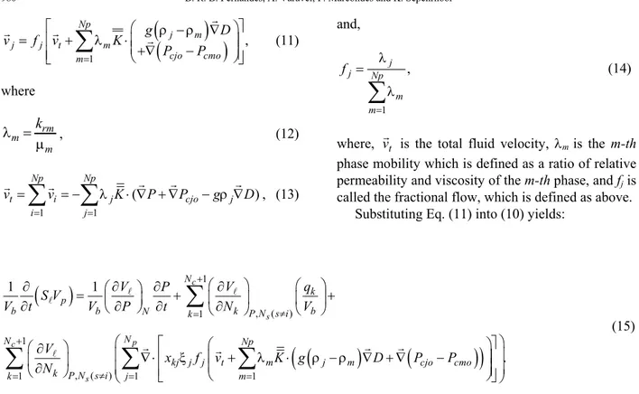
Fig. 2 shows the flow chart of the procedure used in the UTCOMP simulator for the implementation of the Watts’ formulation. As we can see in this figure, pressure is evaluated first; then, an iterative proce-dure is used to evaluate the saturations.
START
Evaluate pressure at the new time-step
Evaluate total velocity
Evaluate residues and derivatives for phase j
Solve the saturation differences and evaluate the new saturations
Evaluate the last saturation as one minus the summation of the other saturations
Evaluate the number of moles at the new time-step
Perform flash calculation and all properties at the new time-step
END j=1
j < NP-1 false
True Newton's Convergence reached? No Yes j=j+1 START
Evaluate pressure at the new time-step
Evaluate total velocity
Evaluate residues and derivatives for phase j
Solve the saturation differences and evaluate the new saturations
Evaluate the last saturation as one minus the summation of the other saturations
Evaluate the number of moles at the new time-step
Perform flash calculation and all properties at the new time-step
END j=1
j < NP-1 false
True Newton's Convergence reached? No Yes j=j+1
Figure 2: Flow chart for Watts’ formulation.
The mobilities, the densities, and the mole frac-tion of each component in each phase at each grid-block interface are evaluated using a one-point up-wind interpolation function. A total variation di-minishing (TVD) method using the Koren’s flux limiter (Koren, 1993; Liu et al., 1995; Fernandes et al., 2013) was also implemented for solving the saturation equations in the relative permeabilities and phase compositions. In this situation, as a non-linear term is included in the relative permeability due to the flux-limiter, it was treated semi-implicitly using the idea presented by Rubin and Blunt (1991), in which the higher order terms are only considered in the independent term of the linear system. For the one-point upwind implementation, the mobilities are evaluated as:
1
, 1 ,
1 1
1 1/2
, 1 ,
1 if
. if
n n n
j j x j x
n x
j x n n n
j j x j x
x + − + − + + − +
⎧λ Φ >Φ
⎪
λ = ⎨
λ Φ ≤Φ
⎪⎩ (21)
w w w
p w p
V N
S
V V
= =
ξ , (22)
and
(
)
2
1 w
Np
p j
j j
L S V
S
V L
=
⎛ ⎞
− ⎜ ⎟
ξ
⎝ ⎠
= =
⎛ ⎞
⎜ ⎟
⎜ξ ⎟
⎝ ⎠
∑
A A A
A , (23)
where L is the phase mole fraction obtained in the flash in the absence of water.
In this work, relative permeability is modelled by the Corey’s model (Corey, 1986) and capillary pres-sure is modelled according to Chang (1990) as:
(
1)
;φ
= − σ −
⎛ ⎞
φ
= − σ ⎜⎜ ⎟⎟
+
⎝ ⎠
pc
pc
E
cow pc wo w
y
E w cog pc og
y o g
P C S
K
S
P C
K S S
, (24)
where Cpc and Epc are user-input parameters, σ is the
interfacial tension between the two phases and
S
denotes a normalized saturation.
For both approaches used in this work, one needs to solve the same number of variables. All variables are listed in Table 1. Also, Table 1 shows some func-tional relations for some of the variables used in this work.
Table 1: List of functional relations.
Variable IMPEC IMPSAT No. of Equations
per grid block
Vp Eq. (6) Eq. (6) 1
Sj Eqs. (22-23) Eq. (16) Np
ξj EOS EOS Np
xij EOS EOS Nc(Np-1)
krj Corey model (1986) Corey model (1986) Np
μj Lorenz (1964) et al. Lorenz (1964) et al. Np
P Eq. (20) Eq. (20) 1
Pcj Chang (1990) Chang (1990) Np-1
ρj EOS EOS Np
qi Well model Well model Nc+1
Ni Eq. (19) Eq. (19) Nc+1
Total NcNp+6Np +Nc+3
The phase appearance for the IMPEC and IMPSAT approaches developed in this work is treated only by the phase stability test, as described earlier. Also, the phase disappearance for the IMPEC approach is based
on the phase stability test. However, for the IMPSAT approach, because phase saturation can be computed as zero or negative during the solution of Eq. (16), we have to couple the stability test with another ap-proach. In this case, if the solution of Eq. (16) pro-duces a negative saturation, we set that saturation to zero. When a negative saturation is calculated, it means that the phase disappears for that time-step. Setting saturation to zero is a common approach used for some fully implicit approaches; see Coats (1980), for instance.
RESULTS AND DISCUSSION
In this section, we investigate the numerical solu-tions, as well as the performance in terms of CPU time of the Watts’ formulation implemented in this work and the original IMPEC approach of the UTCOMP simulator. The comparison studies were carried out by empirically setting the maximum al-lowable time-step for various case studies, which did not produce oscillatory results for both investigated formulations.
The first case investigated is CO2 injection in an
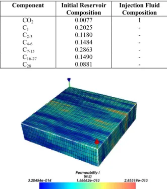
isotropic heterogeneous reservoir. All reservoir data used for this case are shown in Table 2. The water is not considered in flash calculations and is not injected in the reservoir for this case. The water mole numbers are estimated by density and initial saturation.
The components, the initial fluid compositions, and the injected fluid compositions are shown in Table 3.
Table 2: Reservoir data - Case 1.
Property Value
Length, Width and Height 152.4 m, 304.8 m and 6.096 m
Porosity 0.25
Initial Water Saturation 0.25
Initial Pressure 7.58 MPa
Permeability in Z direction 9.87x10⁻¹⁵ m2
Formation Temperature 313.71 K
Injector BHP 8.62 MPa
Producer BHP 7.58 MPa
Grid 20x40x1
Table 3: Component data - Case 1.
Component Initial Reservoir Composition
Injection Fluid Composition
CO2 0.0337 0.95
C1 0.0861 0.04999
C2-3 0.1503 0.000002
C4-6 0.1671 0.000002
C7-15 0.3304 0.000002
C16-27 0.1611 0.000002
Brazilian Journal of Chemical Engineering
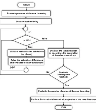
The absolute permeability fields in the x and y di-rections are shown in Fig. 3. In order to better visualize the variation of the permeability fields, Figs. 3b and 3c show two different zooms of the whole scale presented in Fig. 3a.
(a)
(b)
(c)
Figure 3: Permeability in x and y directions. a) Whole scale limits; b) and c) scale zoom.
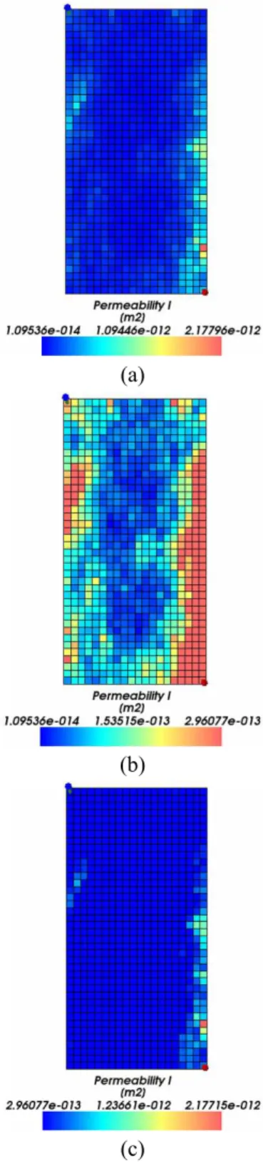
We compare the results of the Watts’ formulation with the original IMPEC formulation of the UT-COMP simulator. The results in terms of oil and gas production are presented in Figs. 4a and 4b, respec-tively. From Fig. 4, we can observe a good agree-ment between the original IMPEC formulation and the Watts’ formulation implemented.
(a)
(b)
Figure 4: Volumetric production rates - Case 1. a) Oil and b) Gas.
In this case, water saturation (volumetric fraction) is lower than the so-called connate saturation (0.25) and hence water cannot flow through the rock pores. Initially, only oil and a mixture of CO2 and light
hydrocarbons injected (gas) are present in the reservoir. As a result, CO2 displaces oil first and
(a) (b)
Figure 5: Second liquid front at 1844 days. a) IMPEC; b) Watts.
The time-steps used by the original UTCOMP ap-proach (IMPEC) and the Watts’ apap-proach are shown in Fig. 6.
Figure 6: Time-step - Case 1.
As we can observe in Fig. 6, the time-steps used by the Watts’ formulation were larger than those of the IMPEC formulation for the entire simulation. Due to the computational time spent for the solution of the linear system equations for the saturations, the Watts’ formulation is more expensive per time-step. However, the large time-steps used by the Watts’ formulation allowed this formulation to be less ex-pensive in terms of CPU time than the IMPEC for-mulation. This fact can be seen in Table 4, which shows the total CPU time used by both formulations. From this table, we observe that Watts’ formulation is about two times faster than the IMPEC formula-tion. We also check the formulations’ performances by doubling the number of gridblocks in each direc-tion. As we can see in Table 4, the speed-up ratio of the Watts’ formulation is improved when the number of gridblocks is doubled in each direction.
Table 4: CPU time comparison - Case 1.
Grid CPU time for IMPEC (s)
CPU time for Watts (s)
Speed-up ratio
20x40 220.21 110.45 1.99 40x80 2829.46 1094.24 2.59
Case 2 is similar to Case 1, but we replaced the upwind interpolation function by a third-order TVD interpolation function. Figs. 7a and 7b show the volu-metric rate of oil and gas, respectively, and Fig. 8 presents the second liquid saturation front at 1844 days. Once again, the Watts’ formulation results are in good agreement with the IMPEC formulation. Despite the large difference when comparing the production rates for TVD solution (Figure 7) with that of upwind solution (Figure 4), the phase behavior obtained was similar for the two cases (the third phase does appear).
(a)
(b)
Figure 7: Volumetric production rates - Case 2. a) Oil and b) Gas.
Brazilian Journal of Chemical Engineering
(a) (b) Figure 8: Second liquid front at 1844 days. a) IMPEC;
b) Watts.
Figure 9: Time-step comparison - Case 2.
Table 5: CPU time comparison - Case 2.
Formulation CPU time (s) Speed-up ratio
IMPEC 980.95 1
Watts 482.44 2.03
Case 3 refers to a WAG (water-alternating gas) process in a heterogeneous reservoir. For this case study, in each cycle, we first inject CO2, and then
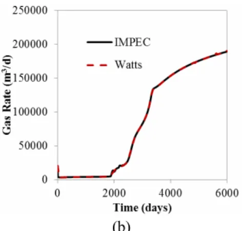
water. Each fluid is injected at a fixed pressure over the course of ten days. The total simulation time is 280 days, which corresponds to fourteen cycles. Tables 6 and 7 present the reservoir data set and the initial and the injected fluid compositions, respec-tively, employed for this case study. Two hydrocar-bon phases were considered in this case and water still is not accounted for in the flash calculations. The absolute permeability field in the x and y directions is shown in Figure 10, while the permeability in the z direction is constant and equal to 7.89x10⁻¹⁵ m2 (8 mD). For this case study, the upwind scheme was used to obtain the solution for both formulations. Figures 11a and 11b present the oil and gas volumetric rates,
respectively, and Fig. 12 shows the oil saturation front at 254 days using a 100x100x5 Cartesian grid.
Table 6: Reservoir data – Case 3.
Property Value
Length, width and thickness
146.30 m, 146.30 m and 14.48 m
Porosity 0.163
Initial Water Saturation 0.65
Initial Pressure 9.65 MPa
Formation Temperature 333.15 K
Injector BHP 10 MPa
Producer BHP 6.89 MPa
Grid 100x100x5
Table 7: Component data – Case 3.
Component Initial Reservoir Composition
Injection Fluid Composition
CO2 0.0077 1
C1 0.2025 -
C2-3 0.1180 -
C4-6 0.1484 -
C7-15 0.2863 -
C16-27 0.1490 -
C28 0.0881 -
Figure 10: Absolute permeability in x and y direc-tions – Case 3.
(b)
Figure 11: Volumetric production rates - Case 3. a) Oil and b) Gas.
(a)
(b)
Figure 12: Oil saturation front at 254 days - Case 3. a) IMPEC; b) Watts.
The time-steps used by both formulations are shown in Fig. 13 and the total CPU time and the speed-up ratio are presented in Table 8. From the figures, we can observe that the average time-step used by Watts’
formulation is approximately three times larger than that used by the IMPEC approach. This average time-step results in a speed-up ratio of 1.7, as we can see in Table 8. In general, at the beginning of each cycle, the time-step size is very close to the minimal time-step designed for the whole simulation. This approach should be in favor of the IMPEC formulation.
Figure 13: Time-step comparison - Case 3. Table 8: CPU time comparison - Case 3.
Formulation CPU time (s) Speed-up ratio
IMPEC 4372.53 1
Watts 2571.68 1.70
The fourth case study is another WAG process, but now a homogeneous reservoir is tested. Capillary pressure is now included in order to check the algo-rithm performance when this physical phenomenon is relevant. Except for absolute permeabilities, all of the previous data presented in Tables 6 and 7 were used. The absolute permeabilities in the x and y-directions are set to 1.97x10⁻¹³ m2, and the one in the z-direction is equal to 9.87x10⁻¹⁴ m2. We use an 80x80x5 grid, and the process is simulated for 100 days. The oil and gas rates are presented in Figs. 14a and 14b, respec-tively. Once again, we can observe a good match be-tween the results of the two approaches compared.
Brazilian Journal of Chemical Engineering
(b)
Figure 14: Volumetric production rates - Case 4. a) Oil and b) Gas.
The time-step comparison is shown in Fig. 15. From this figure, we can verify that the maximum time-step employed by the Watts’ formulation is about two times larger than the one used by the IMPEC ap-proach. It is important to mention that the time-step ratio, aforementioned, is relevant for only the second and third cycles, as we can verify from Fig. 15.
Figure 15: Time-step comparison - Case 4. Table 9 presents the CPU time and the speed-up ratio obtained for case 4. From this table, we can verify that the performance of Watts’ formulation is worse compared to the previous cases, but it still performs better than the IMPEC approach. Further investigation of the current Watts’ implementation needs to be performed when still more complicated physical parameters are involved.
Table 9: CPU time comparison - Case 4.
Formulation CPU time (s) Speed-up ratio
IMPEC 20379.88 1
Watts 15119.04 1.35
The last case study refers to a 2D gas flood with twenty-five components. Only two-hydrocarbon phases
and an immobile aqueous phase are considered. The purpose of this case is to see how Watts’ approach will perform with a large number of components by looking at the impact of expensive flash calculations over the simulation performance. Tables 10 and 11 show the reservoir data and the initial and the in-jected fluid compositions, respectively. It is worth-while to mention that all the components equal or higher than C25+ have identical physical properties.
The main goal here was to verify the performance of the compared approaches with a very large number of components.
Table 10: Reservoir data – Case 5.
Property Value
Length, width and thickness
609.6 m, 609.6 m and 6.1 m
Absolute permeability in x, y, and z-directions
9.87x10⁻¹⁴ m2, 9.87x10⁻¹⁴ m2 and 9.87x10⁻¹⁵ m2
Porosity 0.25
Initial Water Saturation 0.25
Initial Pressure 19.65 MPa
Formation Temperature 400 K
Injector BHP 20 MPa
Producer BHP 16.55 MPa
Grid 40x40x1
Table 11: Component data – Case 5.
Component Initial Reservoir Composition
Injection Fluid Composition
CO2 0.0077 0.01
C1 0.2025 0.65
C2-3 0.1180 0.30
C4-6 0.1484 0.04
C7-14 0.2863 -
C15-24 0.1490 -
Other components (C25+)
0.0063
-
Figure 16 shows the oil and gas volumetric rates. From this figure, we can see a good match for oil and gas volumetric rates for both approaches.
(b)
Figure 16: Volumetric production rates - Case 5. a) Oil and b) Gas.
The time-steps used by both approaches are shown in Fig. 17. From this figure, we can verify that Watts’ formulation was able to handle this case study with several components using much large time-steps compared to the IMPEC formulation.
Figure 17: Time-step comparison - Case 5.
Table 12 presents the total CPU time and speed-up ratio for both approaches. We also show the speed-up ratios when gridblocks in each direction are doubled. From this table, we can infer that Watts’ formulation is about 2.25 times faster than the IMPEC approach.
Table 12: CPU time comparison - Case 5.
Grid CPU time for IMPEC (s)
CPU time for Watts (s)
Speed-up ratio
40x40 5077.58 2260.12 2.25 80x80 55782.76 28942.05 1.93
This suggests that, for a large number of compo-nents, the Watts’ formulation should be used instead of the IMPEC approach. However, when the number of gridblocks is increased, the speed-up ratio de-creased to 1.93. Although the Watts’ formulation
performance decreased when the gridblocks are in-creased, this formulation is still about 2 times faster than the IMPEC approach.
CONCLUSIONS
In this work, we implemented the Watts’ formula-tion for composiformula-tional reservoir simulaformula-tion using Cartesian grids. This formulation was included into the UTCOMP simulator. Also, two interpolation functions for evaluating the physical properties at each interface of the control volume were imple-mented: UDS and a third-order TVD scheme. At least for the case studies investigated, the speed-up ratio of the Watts’ formulation did not change when the TVD and UDS schemes were used. For most of the case studies tested, the Watts’ formulation implemented in this work was around two times faster than the origi-nal IMPEC formulation of the UTCOMP simulator. We also verify, for some case studies, that the per-formance of Watts’ formulation persists when the mesh is refined. It was also confirmed that the new implemented formulation is more efficient than the IMPEC for cases with a large number of components.
NOMENCLATURE
cf Rock compressibility Pa-1
g Gravity m d-2
f Fractionary flow or fugacity
for the equilibrium constraint
K Absolute permeability tensor
m2
r
k Relative permeability L Phase mole fraction N Number of moles, mol
c
N Number of components
p
N Number of phases
P Pressure Pa
q Well mole rate mol d-1
S Saturation
t Time s
b
V Bulk volume m3
p
V Pore volume m3
t
V Total fluid volume m3
tk
V Total fluid partial molar volume
m3 mol-1
Brazilian Journal of Chemical Engineering k
VA Phase partial molar volume m3 mol-1
vG Velocity vector m d-1
x Component mole fraction in each phase
Greek Letters
ξ Mole density mol m-3
ρ Mass density kg m-3
σ Interfacial tension N m-1
φ Porosity
λ Phase mobility Pa-1 d-1
Φ
Hydraulic potential Paμ Viscosity Pa d
t
Δ Time step size d
x
Δ Spatial step size in the x direction
m
y
Δ Spatial step size in the y direction
m
z
Δ Spatial step size in the z direction
m
Superscripts
n Previous time step level n+1 New time step level
Subscripts
b Back interface B Back control volume e East interface E East control volume f Front interface F Front control volume
g Gas phase
i Control volume
j Phase
k Component
ℓ Phase
n North interface N North control volume
o Oil phase
P Control volume
r Reference phase
s South interface S South control volume
t Total
w Water component/phase or west interface
W West control volume
ACKNOWLEDGMENTS
The authors would like to acknowledge the Abu Dhabi National Oil Company for the financial support for this work. We would like to thank Dr. Chowdhury K. Mamum for his comments on this manuscript. Also, the third author would like to thank the CNPq (The National Council for Scientific and Technologi-cal Development of Brazil) for financial support through the grant No. 305415/2012-3. Finally, we would like thank the ESSS (Engineering Scientific Software Simulating) for proving the Kraken® to pre and post-processing the results.
REFERENCES
Ács, G., Doleschall, S. and Farkas, E., General pur-pose compositional model. SPE Journal, 25(4), p. 543-553 (1985).
Branco, C. M. and Rodriguez, F., A Semi-implicit formulation for compositional reservoir simula-tion. SPE Advanced Technology Series, 4(1), p. 171-177 (1996).
Cao, H., Development of Techniques for General Purpose Simulators. Ph.D. Thesis, Stanford Uni-versity (2002).
Chang, Y.-B., Development and Application of an Equation of State Compositional Simulator. Ph.D. Dissertation, The University of Texas at Austin, Austin Texas (1990).
Chang, Y.-B., Pope, G. A. and Sepehrnoori, K., A higher-order finite-difference compositional simu-lator. Journal of Petroleum Science and Engineer-ing, 5(1), p. 35-50 (1990).
Coats, K. H., An equation of state compositional model. SPE Journal, 20(5), p. 363-376 (1980). Corey, A. T., Mathematics of immiscible fluids in
porous media. Water Resources Publication, Little-ton, CO (1986).
Fernandes, B. R. B., Marcondes, F. and Sepehrnoori, K., Investigation of several interpolation func-tions for unstructured meshes in conjunction with compositional reservoir simulation. Numerical Heat Transfer Part A, Applications, 64(12), p. 974-993 (2013).
Jhaveri, B. S. and Youngren, G. K., Three-parameter modification of the Peng-Robinson equation of state to improve volumetric prediction. SPE Res-ervoir Engineering, 3(3), p. 1033-1040 (1988). Kaasschieter, E. F., Solving the Buckley-Leverett
Kendall, R. P., Morrell, G. O., Peaceman, D. W. and Watts, J. W., Development of a multiple applica-tion reservoir simulator for use on a vector com-puter. SPE Middle East Oil technical conference. SPE, Manama, Bahrain (1983).
Koren, B., A Robust Upwind Discretization Method for Advection, Diffusion and Source Terms. In: C. B., Vreugdenhil, and B., Koren, (Eds.), Numerical Methods for Advection-Diffusion Problems. Notes on Numerical Fluid Mechanics, vol. 45, p. 117-138, Vieweg, Braunschweig (1993).
Liu, L., Delshad, M., Pope, G. A. and Sepehrnoori, K., Application of higher-order flux-limited meth-ods in compositional simulation. Transport in Porous Media, 16(1), p. 1-29 (1994).
Lohrenz, J., Bray, B. G. and Clark, C. R., Calculating viscosities of reservoir fluids from their composi-tions. Journal of Petroleum Technology, 16(10), p. 1171-1176 (1964).
Mehra, A. R., Heidemann, R. A. and Aziz, K., An accelerated successive substitution algorithm. Ca-nadian Journal of Chemical Engineering, 61(4), p. 590-596 (1983).
Michelsen, J. L., The isothermal flash problem. Part I. Stability, Fluid Phase Equilibria, 9(1),
p. 1-19 (1982).
Peng, D. Y. and Robinson, D. B., The characteriza-tion of the heptanes and heavier fraccharacteriza-tions for the GPA Peng-Robinson programs. Gas Processors Association (1978).
Perschke, D. R., Equation of State Phase Behavior Modelling for Compositional Simulator. Ph.D. Thesis, The University of Texas at Austin, Austin, Texas (1988).
Runbin, B. and Blunt, M. J., Higher-order implicit flux limiting schemes for black-oil simulation. SPE Symposium on Reservoir Simulation, SPE, Anaheim, USA, p. 219-229 (1991).
Spillette, A. G., Hillestad, J. G. and Stone, H. L., A high-stability sequential solution approach to reservoir simulation. Fall Meeting of the Society of Petroleum Engineers of AIME. SPE, Las Ve-gas, Nevada, USA (1973).
Trangenstein, J. A., Customized minimization tech-niques for phase equilibrium computations in res-ervoir simulation. Chemical Engineering Science, 42(12), p. 2847-2863 (1988).