ISSN 0101-8205 www.scielo.br/cam
Semiconductors and Dirichlet-to-Neumann maps
ANTONIO LEITÃO
Department of Mathematics, Federal University of St. Catarina 88040-900 Florianopolis, Brazil
E-mail: [email protected]
Abstract. We investigate the problem of identifying discontinuous doping profiles in semi-conductor devices from data obtained by the stationary voltage-current (VC) map. The related inverse problem correspond to the inverse problem for the Dirichlet-to-Neumann (DN) map with partial data.
Mathematical subject classification: 35R30, 82D37, 35Q60. Key words:semiconductors, inverse doping, bipolar model.
1 Introduction
In this paper we investigate the problem of identifying discontinuous doping profiles in semiconductor devices from data obtained by the VC map for the linearized stationary bipolar model (close to equilibrium). Two different methods of data acquisition are considered:
1) Current flow measurements through a contact;
2) Pointwise measurements of the current density.
The related inverse problems correspond to the inverse problem for the DN map with partial data.
We propose a framework to handle the inverse problems and analyze relevant properties of the parameter-to-output maps. Moreover, we present a numerical experiment for the case of pointwise measurements of the current density.
The paper is outlined as follows: In Section 2 we present the transient end stationary drift diffusion equations. In the Section 3 we introduce the VC map and derive the underlying model for the analysis presented in this paper, namely thelinearized stationary bipolar case (close to equilibrium). Two inverse prob-lems corresponding to different data acquisition procedures are introduced in Section 4. Some regularity properties of the related parameter-to-output maps are verified in this section. In Section 5 we present some numerical results for a level set type iterative method and pointwise measurements of the current den-sity. This experiment indicate that a single measurement may suffices to identify the doping profile.
2 Drift diffusion equations The transient model
The basic semiconductor device equations consist of the Poisson equation (1a), the continuity equations for electrons (1b) and holes (1c), and the current relations for electrons (1d) and holes (1e).
div(ǫ∇V)=q(n−p−C) in×(0,T) (1a)
divJn =q(∂tn+R) in×(0,T) (1b) divJp=q(−∂tp−R) in×(0,T) (1c)
Jn =q(Dn∇n−μnn∇V) in×(0,T) (1d)
Jp =q(−Dp∇p−μpp∇V) in×(0,T) . (1e)
The function R has the form R = R(n,p,x)(np − n2i) and denotes the recombination-generation rate(ni is the intrinsic carrier density). Thebandgap is relatively large for semiconductors (gap between valence and conduction band), and a significant amount of energy is necessary to transfer electrons from the valence and to the conduction band. This process is called genera-tion of electron-hole pairs. On the other hand, the reverse process corresponds to the transfer of a conduction electron into the lower energetic valence band. This process is called recombination of electron-hole pairs. In our model these phenomena are described by the recombination-generation rate R. Frequently adopted in the literature are the Shockley Read Hall model (RS R H) and the Auger
model (RAU), defined by
RS R H :=
τp(n+ni)+τp(p+ni)
−1 ,
RAU := Cnn+Cpp,
whereCn,Cp,τnandτpare positive constants (see Appendix).
The functionC(x)models a preconcentration of ions in the crystal, soC(x)=
C+(x)−C−(x) holds, whereC+ and C− are concentrations of negative and
positive ions respectively. In those subregions ofin which the
preconcentra-tion of negative ions predominate (P-regions), we haveC(x) <0. Analogously, we define the N-regions, whereC(x) > 0 holds. The boundaries between the
P-regions and N-regions (whereCchange sign) are calledpn-junctions. In the sequel we turn our attention to the boundary conditions. We assume the boundary∂ofto be divided into two nonempty disjoint parts: ∂ = ∂N ∪ ∂D. The Dirichlet part of the boundary∂Dmodels the Ohmic con-tacts, where the potentialV as well as the concentrationsnandpare prescribed. The Neumann part ∂N of the boundary corresponds to insulating surfaces, thus a zero current flow and a zero electric field in the normal direction are prescribed. The Neumann boundary conditions for system (1a)–(1e) read:
∂V
∂ν(x,t)= ∂n
∂ν(x,t)= ∂p
∂ν(x,t)=0, ∂N× [0,T]. (2)
imposed:
V(x,t)=VD(x,t)=U(x,t)+Vbi(x)=U(x,t)+UT ln
nD(x)
ni
(3a)
n(x,t)=nD(x)= 1 2
C(x)+
q
C(x)2+4ni2
(3b)
p(x,t)= pD(x)= 1 2
−C(x)+ q
C(x)2+4n2i
. (3c)
Here the functionU(x,t)denotes the applied potential, the constantUT repre-sents the thermal voltage, andVbi is given logarithmic function [4]. We shall consider the simple situation∂D = Ŵ0∪Ŵ1, which occurs, e.g., in a diode. The disjoint boundary partsŴi,i = 0,1, correspond to distinct contacts. Dif-ferences inU(x)between different segments of∂D correspond to the applied bias between these two contacts. Moreover, the initial conditionsn(x,0) ≥ 0,
p(x,0)≥0 have to be imposed.
The stationary model
In this paragraph we turn our attention to the stationary drift diffusion equations. We disconsider the thermal effects and assume further ∂n/∂t = ∂n/∂t = 0. Thus, thestationary drift diffusion modelis derived from (1a)–(1e) in a straight-forward way. Next, motivated by the Einstein relations Dn = UTμn and Dp = UTμp (a standard assumption about the mobilities and diffusion coef-ficients), one introduces the so-calledSlotboom variables u andv, which are
related to the originalnand pvariables by the formula:
n(x)=niexp
V(x)
UT
u(x) , p(x)=niexp
− V(x) UT
v(x) . (4)
For convenience, we rescale the potential and the mobilities, i.e.
V(x) ← V(x)
UT
, μn ← qUTμn, μp ← qUTμp.
Next we write the stationary drift diffusion equations in terms of(V,u, v)
λ21V = δ2 eVu−e−Vv−C(x) in (5a)
divJn = δ4Q(V,u, v,x) (uv−1) in (5b) divJp= −δ4Q(V,u, v,x) (uv−1) in (5c)
V = VD = U+Vbi on∂D (5d)
u= uD = e−U on∂D (5e)
v= vD = eU on∂D (5f)
∇V ∙ν= Jn∙ν = Jp∙ν = 0 on∂N, (5g)
where λ2 := ǫ/(qUT) is the Debye length of the device, δ2 := ni and the functionQis defined implicitly by the relationQ(V,u, v,x)=R(n, p,x).1
One should notice that, due to the thermal equilibrium assumption, it follows np=n2i, and the assumption of vanishing space charge density givesn−p−C =
0, forx ∈ ∂D. This fact motivates the boundary conditions on the Dirichlet part of the boundary.
It is worth mentioning that, in a realistic model, the mobilities μn and μp usually depend on the electric field strength|∇V|. In what follows, we assume thatμnandμpare positive constants. This assumption simplifies the subsequent analysis, allowing us to concentrate on the inverse doping problems. As a matter of fact, this dependence could be incorporated in the model without changing the results described in the sequel.
Existence and uniqueness of solutions for system (5) can only be guaranteed for small applied voltages. Therefore, it is reasonable to consider, instead of this system, its linearized version around the equilibrium pointU ≡ 0. We shall return to this point in the next section, where the VC map is introduced.
3 A simplified model
In the sequel we make some simplifying assumptions on the stationary drift diffusion equations introduced in Section 2 and derive a special case which will serve as underlying model for the inverse problem investigated in Section 4.
The linearized stationary drift diffusion equations (close to equilibrium)
We begin this paragraph by introducing the thermal equilibrium assumption for the stationary drift diffusion equations. This is a previous step to derive a linearized system of stationary drift diffusion equations (close to equilibrium).
The thermal equilibrium assumption refers to the condition in which the semi-conductor is not subject to external excitations, except for a uniform temperature, i.e. no voltages or electric fields are applied. It is worth noticing that, under the thermal equilibrium assumption, all externally applied potentials to the semicon-ductor contacts are zero (i.e. U(x) =0). Moreover, the thermal generation is perfectly balanced by recombination (i.e. R=0).
If the applied voltage satisfiesU =0, one immediately sees that the solution of system (5a)–(5g) simplifies to(V,u, v)=(V0,1,1), whereV0solves
λ21V0= eV0 −e−V0−C(x) in (6a)
V0= Vbi(x) on ∂D (6b)
∇V0∙ν= 0 on∂N. (6c)
In the bipolar model discussed below we shall be interested in the linearized drift diffusion system at the equilibrium. Keeping this in mind, we compute the Gateaux derivative of the solution of system (5a)–(5g) with respect to the voltage U at the pointU ≡0 in the directionh. This directional derivative is given by the solution(Vˆ,uˆ,v)ˆ of
λ21Vˆ =eV0uˆ+e−V0vˆ+(eV0 +e−V0)Vˆ in (7a)
div(μneV
0
∇ ˆu)= Q0(V0,x)(uˆ + ˆv) in (7b) div(μpe−V
0
∇ ˆv)= Q0(V0,x)(uˆ+ ˆv) in (7c)
ˆ
V = h on∂D (7d)
ˆ
u= −h on∂D (7e)
ˆ
v= h on∂D (7f)
Linearized stationary bipolar case (close to equilibrium)
In this paragraph we present a special case, which plays a key rule in the modeling inverse doping problems related tocurrent flowmeasurements.
The following discussion is motivated by the stationary VC map
6C : H3/2(∂D) → R.
U 7→
Z
Ŵ1
(Jn+Jp)∙νds
Here (V,u, v) is the solution of system (5) for an applied voltage U. This operator models practical experiments wherevoltage-current dataare available, i.e. measurements of the averaged outflow current density onŴ1⊂∂D.
The linearized stationary bipolar case (close to equilibrium)corresponds to the model obtained from the drift diffusion equations (5) by linearizing the VC map atU ≡ 0. This simplification is motivated by the fact that, due to hys-teresis effects for large applied voltage, the VC map can only be defined as a single-valued function in a neighborhood ofU = 0. Moreover, the following simplifying assumptions are also taken into account:
A1) The electron mobilityμnand hole mobilityμpare constant;
A2) No recombination-generation rate is present, i.e. R=0 (or Q0=0). An immediate consequence of our assumptions is the fact that the Poisson equation and the continuity equations decouple. Indeed, from (7) we see that the Gateaux derivative of the VC map6C at the pointU = 0 in the direction h∈ H3/2(∂
D)is given by the expression
6C′(0)h = Z
Ŵ1
μneVbiuˆν−μpe−Vbivˆν
ds, (8)
where(uˆ,v)ˆ solve
div(μneV
0
∇ ˆu)= 0 in (9a)
div(μpe−V
0
∇ ˆv)= 0 in (9b)
ˆ
u = −h on∂D (9c)
ˆ
v = h on∂D (9d)
andV0is the solution of the equilibrium problem (6); see Lemma 1.
Notice that the solution of the Poisson equation can be computed a priori, since it does not depend onh. The application6′C(0)maps the Dirichlet data for(uˆ,v)ˆ
to a weighted sum of their Neumann data and can be compared with the DN map in theElectrical Impedance Tomography(EIT).
4 Inverse Problems for Semiconductors
We begin this section verifying that the stationary VC map6C, introduced in
Section 3, is well defined in a suitable neighborhood ofU =0.
Lemma 1 [[5], Proposition 3.1]. In (5), for each applied voltage U ∈ Br(0)
⊂ H3/2(∂
D)with r > 0 sufficiently small, the current J ∙ν ∈ H1/2(Ŵ1) is uniquely defined. Furthermore,6C : H3/2(∂D) → H1/2(Ŵ1)is continuous and continuously differentiable in Br(0). Moreover, it’s derivative in direction h∈ H3/2(∂D)is given by the operator6C′ (0)defined in(8).
As a matter of fact, we can actually prove that, since (uˆ,v)ˆ in (9) depend
continuously (in H2()2) on the boundary data U ∈ H3/2(∂
D), it follows from the boundedness and compactness of the trace operator γ : H2() →
H1/2(Ŵ
1)that6C′ (0)is a bounded and compact operator.
Lemma 1 establishes a basic property to consider the inverse problem of recon-structing the doping profileCfrom the VC map. In the sequel we shall consider two possible inverse problems for this map.
Current flow measurements through a contact
In this first inverse problem we assume that, for eachC, the output is given by 6C′(0)Uj for someUj. A realistic experiment corresponds to measure, for given
Uj
N
j=1, withkUjksmall, the outputs
6C′(0)Uj | j=1,∙ ∙ ∙ ,N
6C′(0)we derive the following abstract formulation of the inverse doping profile
problem for the VC map:
F(C) = Y, (10)
where
1) Uj
N
j=1⊂H3/2(∂D)are fixed voltage profiles satisfyingUj|Ŵ1 =0;
2) Parameter: C =C(x) ∈ L2()=:X;
3) Output: Y =
6C′(0)Uj N
j=1∈RN =:Y; 4) Parameter-to-output map: F :X→Y.
The domain of definition of the operatorF is
D(F) :=
C ∈L∞();Cm ≤C(x)≤CM, a.e. in ,
whereCm andCM are suitable positive constants.
The inverse problem described above corresponds to the problem of identify-ing the dopidentify-ing profileC from the linearized stationary VC map atU =0 (see bipolar case in Section 3).
The non-linear parameter-to-output operator F is well defined and Fréchet differentiable in its domain of definition D(F). This assertion follows from
standard regularity results in PDE theory (see, e.g., [4], Propositions 2.2 and 2.3). It is worth noticing that the solution of the Poisson equation can be computed a priori. The remaining problem (coupled system (9) for(uˆ,v)ˆ ) is quite sim-ilar to the problem of EIT. In this inverse problem the aim is to identify the conductivityq =q(x)in the equation:
−div(q∇u) = f in ,
from measurements of theDirichlet-to-Neumann map, which maps the applied voltage u|∂ to the electrical flux quν|∂. The application 6C′(0) maps the Dirichlet data foruˆ andvˆ to the weighted sum of their Neumann data. It can
Pointwise measurements of the current density
In the sequel, we investigate a different inverse problem related to the VC map. Differently from the previous paragraph, we shall assume that the VC operator maps the Dirichlet data foruˆ andvˆ in (9) to the sum of their Neumann data, i.e.
6C :H3/2(∂D) → H1/2(Ŵ1) U 7→ (Jn+Jp)∙ν|Ŵ1
where functionsV,uˆ,vˆ, Jn, JpandU have the same meaning as in Section 3. It is immediate to observe that the Gateaux derivative of the VC map6Cat the pointU =0 in the directionh ∈ H3/2(∂
D)is given by
6C′(0)h= μneVbiuˆν−μpe−Vbivˆν
|Ŵ1, (11)
where(uˆ,v)ˆ solve system (9). Notice that, for each applied voltageU, the VC map associates a scalar valued function defined onŴ1. In this case, the outputs
6C′(0)Uj are in a data space which is larger than in the case of current flow measurements.
Again we can derive an abstract formulation of type (10) for the inverse doping profile problem for the linearized stationary VC map with pointwise measure-ments of the current density. The only difference to the framework described in the previous paragraph concerns the definition of the Hilbert spaceY, which is now defined by:
3’) Output: Y =
6C′(0)Uj N
j=1∈ L2(Ŵ1)
N =:Y;
The domain of definition of the operatorF, remains unaltered.
It is immediate to observe that the model concerning current flow measure-ments carries less information about the unknown parameter than the model related to pointwise measurements does. In so far, the inverse problem related with the first measurement type is harder to solve.
5 A numerical experiment
In the sequel we consider the bipolar model introduced in Section 3. It follows from the assumption Q = 0 that the Poisson equation (6a) and the continuity equations (9a), (9b) decouple. The inverse doping profile problem corresponds to the identification ofC = C(x) from pointwise measurements of the total
current densityJ at the contactŴ1, namely
J|Ŵ1 =(Jn+Jp)|Ŵ1 = μneVbiuˆν−μpe−Vbivνˆ
|Ŵ1
(compare with the Gateaux derivative of the VC map6C at the pointU = 0 in (8)). Here(V0,uˆ,v)ˆ solve, for each applied voltageU, the system (6), (9), withhsubstituted byU.
Notice that we can split the inverse problem in two parts: First we define the functionγ (x):=eV0(x),x ∈, and solve the parameter identification problem
div(μnγ∇ ˆu)=0 in
ˆ
u= −U(x) on∂D
∇ ˆu∙ν =0 on∂N
div(μpγ−1∇ ˆv)=0 in
ˆ
v=U(x) on∂D
∇ ˆv∙ν=0 on∂N (12)
forγ, from measurements of(μnγuˆν−μpγ−1vν)ˆ |Ŵ1. The second step consists
in the determination ofC in
C(x) = γ (x)−γ−1(x)−λ21(lnγ (x)) , x ∈ .
Since the evaluation ofC fromγ can be explicitely performed in a stable way,
we shall focus on the problem of identifying the function parameterγ in (12).
Summarizing, the inverse doping profile problem in the linearized bipolar model for pointwise measurements of the current density reduces to the identi-fication of the parameterγ in (12) from measurements of the DN map
3γ : H3/2(∂
D) → H1/2(Ŵ1) .
U 7→ μnγuˆν−μpγ−1vˆν
|Ŵ1
If we take into account the restrictions imposed by the practical experiments described in Section 4, it follows:
ii) The identification ofγ has to be performed from a finite number of
mea-surements, i.e. from the data
(Uj, 3γ(Uj)) N j=1∈
H3/2(Ŵ0)×H1/2(Ŵ1)N. (13) For this experiment concerning pointwise measurements of the current density, we assume that only one measurement is available, i.e. N = 1 in (13). What concerns the numerical implementation, we applied an iterative method of level set type to solve the identification problem forγ in (12) (see [19, 15, 20]). The
domain⊂R2is the unit square, and the boundary parts are defined as follows
Ŵ1 := {(x,1); x ∈(0,1)}, Ŵ0 := {(x,0); x ∈(0,1)},
∂N := {(0,y); y ∈(0,1)} ∪ {(1,y); y ∈(0,1)}.
The fixed inputU, is chosen to be a piecewise constant function supported inŴ0
U(x) := (
1, |x−0.5| ≤h 0, else
The doping profile to be reconstructed is shown in Figure 1(a). In Figure 1(b) the voltage sourceU (applied atŴ0) and the corresponding solutionuˆ of (12) are shown. In these pictures, as well as in the forthcoming ones,Ŵ1is the lower left edge andŴ0is the top right edge (the origin corresponds to the upper right corner).
In Figure 2 we present a numerical experiment for the bipolar model with pointwise measurements of the current density. Here exact data is used for the reconstruction of the p-n junction in Figure 1(a). The pictures show plots of the iteration error after 1, 10 and 100 steps of the level set method respectively.
(a)
(b)
Figure 1 – Picture (a) show the doping profiles to be reconstructed in the numerical experiments.
object than the original unknown curve (the P-N junction). Due to the nature of the level set approach, it incorporates in a natural way the assumption thatγ is
Appendix
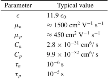
Properties of silicon at room temperature
Parameter Typical value
ǫ 11.9ǫ0
μn ≈1500 cm2V−1s−1
μp ≈450 cm2V−1s−1 Cn 2.8×10⁻³¹cm6/ s Cp 9.9×10⁻³² cm6/ s
τn 10−6s
τp 10−5s
Table 1 – Typical values of main the constants in the model.
Relevant physical constants:
Permittivity in vacuum:ǫ0=8.85×10⁻¹⁴As V−1cm−1; Elementary charge: q =1.6×10⁻¹⁹As.
Acknowledgments. The author was partially supported by the Brazilian Na-tional Research Council CNPq, grants 305823/03-5 and 478099/04-5.
REFERENCES
[1] K. Astala, L. Päivärinta and M. Lassas, Calderón’s inverse problem for anisotropic conductivity in the plane.Comm. Partial Differential Equations,30(2005), 207–224.
[2] L. Borcea, Electrical impedance tomography.Inverse Problems,18(2002), R99–R136.
[3] A. Bukhgeim and G. Uhlmann, Recovering a potential from partial Cauchy data. Comm. Partial Differential Equations,27(2002), 653–668.
[4] M. Burger, H.W. Engl, A. Leitão and P.A. Markowich, On inverse problems for semiconductor equations.Milan Journal of Mathematics,72(2004), 273–314.
[5] M. Burger, H.W. Engl, P.A. Markowich and P. Pietra, Identification of doping profiles in semiconductor devices.Inverse Problems,17(2001), 1765–1795.
[7] S. Busenberg and W. Fang, Identification of semiconductor contact resistivity. Quart. Appl. Math.,49(1991), 639–649.
[8] S. Busenberg, W. Fang and K. Ito, Modeling and analysis of laser-beam-inducted current images in semiconductors.SIAM J. Appl. Math.,53(1993), 187–204.
[9] H.W. Engl, M. Hanke and A. Neubauer, Regularization of Inverse Problems. Kluwer Academic Publishers, Dordrecht (1996).
[10] H.W. Engl, K. Kunisch and A. Neubauer, Convergence rates for Tikhonov regularization of nonlinear ill-posed problems.Inverse Problems,5(1989), 523–540.
[11] W. Fang and E. Cumberbatch, Inverse problems for metal oxide semiconductor field-effect transistor contact resistivity.SIAM J. Appl. Math.,52(1992), 699–709.
[12] W. Fang and K. Ito, Identifiability of semiconductor defects from LBIC images. SIAM J. Appl. Math.,52(1992), 1611–1626.
[13] W. Fang and K. Ito, Reconstruction of semiconductor doping profile from laser-beam-induced current image.SIAM J. Appl. Math.,54(1994), 1067–1082.
[14] W. Fang, K. Ito and D.A. Redfern, Parameter identification for semiconductor diodes by LBIC imaging.SIAM J. Appl. Math.,62(2002), 2149–2174.
[15] F. Frühauf, O. Scherzer and A. Leitão, Analysis of regularization methods for the solu-tion of ill–posed problems involving discontinuous operators. SIAM J Numerical Analysis, 43(2005), 767–786.
[16] H. Gajewski, On existence, uniqueness and asymptotic behavior of solutions of the basic equations for carrier transport in semicinductors. Z. Angew. Math. Mech.,65(1985), 101– 108.
[17] P. Grisvard, Elliptic Problems in Nonsmooth Domains. Pittman Publishing, London, (1985).
[18] V. Isakov, Inverse problems for partial differential equations. Applied Mathematical Sciences, Springer, New York (1998).
[19] A. Leitão and O. Scherzer, On the relation between constraint regularization, level sets, and shape optimization.Inverse Problems,19(2003), L1–L11.
[20] A. Leitão, P.A. Markowich and J.P. Zubelli, On inverse doping profile problems for the voltage-current map. Inverse Problems,22(2006), 1071–1088.
[21] P.A. Markowich, The Stationary Semiconductor Device Equations. Springer, Vienna (1986).
[22] P.A. Markowich, C.A. Ringhofer and C. Schmeiser, Semiconductor Equations. Springer, Vienna (1990).
[23] A.I. Nachman, Global uniqueness for a two-dimensional inverse boundary value problem.
Ann. of Math.,143(1996), 71–96.
[25] W.R. van Roosbroeck, Theory of flow of electrons and holes in germanium and other semiconductors.Bell Syst. Tech. J.,29(1950), 560–607.