ISSN 0101-8205 www.scielo.br/cam
Target identification of buried coated objects
∗FIORALBA CAKONI and DAVID COLTON
Department of Mathematical Sciences, University of Delaware, Newark, Delaware 19716, USA
E-mails: [email protected] / [email protected]
Abstract. We consider the three dimensional electromagnetic inverse scattering problem of determining information about a buried coated object from a knowledge of the electric and magnetic fields measured on the surface of the earth corresponding to time harmonic electric
dipoles as incident fields. We assume that the buried object is a perfect conductor that is (possibly)
partially coated by a thin dielectric layer. No a priori assumption is made on the extent of the coating, i.e. the object can be fully coated, partially coated or not coated at all. We present an
algorithm based on the linear sampling method and reciprocity gap functional for reconstructing the shape of the scattering obstacle together with an estimate of the surface impedance of the
coating.
Mathematical subject classification: Primary: 35R30, 35Q60; Secondary: 35P25; 78A45.
Key words:inverse scattering, mixed boundary conditions, buried objects.
1 Introduction
The use of electromagnetic fields to detect buried objects has a long history and continues to be an active area of research [3], [7], [8]. Of particular interest is the use of such methods to detect chemical waste deposits, examine urban infras-tructure and locate landmines. However, from a practical point of view, there are two main reasons why such imagining problems remain basically unresolved. The first of these problems is the difficulty of distinguishing the scattered field
#689/06. Received: 01/IX/06. Accepted: 01/X/06.
due to the target from the scattered fields due to the earth, the antenna and, in particular, the air-earth interface. A second problem is that the material proper-ties of the target are in general unknown. For example, a landmine can be made of wood, metal or plastic whereas a rusted barrel of chemical waste deposits is typically modeled by a complicated mixed boundary value problem involving a dielectric of unknown permittivity. Due to such problems, traditional methods of imagining such as the use of weak scattering approximations and nonlinear optimization techniques remain problematic.
In recent years a new class of electromagnetic imaging techniques has been developed which has the potential of overcoming the problems mentioned in the above paragraph. These new techniques can be described as “qualitative meth-ods in inverse scattering theory” [4] and have a number of remarkable features which make them attractive for the imaging of buried objects. We will focus our attention on the most popular of these qualitative methods called the linear sampling method [6], [11], [15]. The remarkable feature of the linear sampling method is that 1) it is a linear method that does not ignore multiple scattering effects and 2) it determines the shape of a target without requiring any a pri-ori knowledge of the target’s physical properties. However, until very recently, the implementation of the linear sampling method for a nonhomogeneous back-ground media required a knowledge of the Green’s function for the backback-ground media. This is obviously an unattractive feature if it is desired to use this method for the detection of buried objects, particularly if the scattering effects due to the antenna play a significant role.
when the buried object is a perfect conductor that may be partially coated by a thin dielectric layer. The inverse scattering problem in this case is considerably more complicated than the simple case of a perfect conductor since it is unknown a priori whether or not the target is coated. In particular, the inverse problem is now to not only determine the shape of the target but also whether or not the target is coated and if so the value of the surface impedance of the coating [13]. As in [7], we will consider the case when the electric and magnetic fields are both known on the entire boundary of an absorbing homogeneous region of the background media that is known a priori to contain the target. The case of an object buried in the earth is then handled by assuming that the part of the boundary below the surface of the earth is far away from the incident sources and hence we can assume that the total electric and magnetic fields are very small on this portion of the boundary.
It gives the authors particular pleasure to present our work on the detection of buried objects using electromagnetic fields in the proceedings of a conference dedicated to the twenty fifth anniversary of Alberto Calderon’s seminal paper on the same topic [8]. As is seen by the papers in this volume, Calderon’s paper of 1980 has been a major influence not only on our own work but also on the work of many other mathematicians and scientists working in diverse disciplines. We are happy to be part of this celebration!
2 Formulation of the direct and inverse scattering problems
We consider the scattering of a time-harmonic electromagnetic field of frequency
ω by a scattering object embedded in a piecewise homogeneous background medium inR3. We assume that the magnetic permeabilityμ
0>0 of the
back-ground medium is a positive constant whereas the electric permittivity ǫ(x)
and conductivityσ (x)are piecewise constant. Moreover we assume that for |x| =r > R, for R sufficiently large, σ =0 andǫ(x)=ǫ0. Then the electric
fieldE˜ and magnetic fieldH˜ in the background medium satisfy the time-harmonic
Maxwell’s equations
After an appropriate scaling [12] and elimination of the magnetic field we now obtain the following equation for the electric fieldEin the background medium
curl curlE−k2n(x)E
=0,
where
˜ E= √1
ǫ0
E, k =ǫ0μ0ω2 and n(x)= 1 ǫ0
ǫ(x)+iσ (x) ω
.
Note that the piecewise constant function n(x) satisfies n(x) = 1 for r > R, ℜ(n) > 0 andℑ(n)≥ 0. The surfaces across which n(x)is discontinuous are assumed to be piecewise smooth and closed.
Now let D be a scattering object embedded in the above piecewise homoge-neous background such thatR3\D is connected. We suppose that the boundary ∂D of D is piecewise smooth and denote byν the outward unit normal. Fur-thermore, we assume that the boundary∂D=ŴD∪5∪ŴI is split in two open
disjoint partsŴD andŴI having5as their possible common boundary in∂D.
The domain D is the support of a perfect conductor (possibly a disconnected object) that is partially coated on a portionŴI of the boundary by a very thin
layer of dielectric material. We assume for sake of presentation that the coating is homogeneous. Let the positive constantλ >0 describe the surface impedance of the coating. The incident field is considered to be an electric dipole located at x0∈3with polarization p∈R3given by
Ee(x,x0,p,ks):= i
kscurlxcurlx p
ei ks|x−x0| 4π|x−x0|
(1)
where ks2=k2nsand3is an open surface (to be made precise later on) situated in a layer with constant index of refraction ns. We denote byG(x,x0)the free space
Green’s tensor of the background medium and define Ei(x):= Ei(x,x0,p) =
G(x,x0)p which satisfies
curl curl Ei(x)−k2n(x)Ei(x)= pδ(x−x0) in R3, (2)
whereδdenotes the Dirac distribution. Note that Ei can be written as
where Ebs = Ebs(∙, x0,p) is the electric scattered field due to the background
medium.
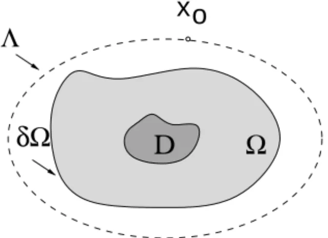
We now consider a bounded domainsuch that D is contained inand the open surface3 is contained inR3
\. Let∂denote the piecewise smooth boundary of . Note that 3 or a portion of 3 may be a subset of∂. We assume the medium inside the domaincontaining the scattering object D is homogeneous with constant index of refraction nb and define kb2 = k2nb (see
Fig. 1).
Λ
δΩ
Ω
xo
D
Figure 1 – Example of the geometry of the scattering problem.
Then the total electric field E =Es+Ei, where Es is the scattered field due to
the obstacle D, satisfies the following equation and mixed boundary conditions:
curl curl E−k2n(x)E =0 inR3\ D∪ {x0}
(4)
ν×E =0 onŴD (5)
ν×curl E−i kbλ(ν×E)×ν =0 onŴI. (6)
In addition, the scattered field Es satisfies the Silver Müller radiation condition
lim
r→∞ curlE s
×x−i kr Es=0 (7)
uniformly inxˆ =x/|x|, r = |x|.
In order to formulate precisely the above scattering problem we are concerned with throughout this paper, we need the following spaces:
H(curl,D) :=
u ∈(L2(D))3: ∇ ×u∈(L2(D))3 L2t(∂D) :=
u ∈(L2(∂D))3:ν∙u =0 on ∂D L2t(ŴI) :=
u|ŴI:u∈ L 2
We introduce the space
X(D, ŴI):= {u ∈ H(curl,D) : ν×u|ŴI ∈ L 2
t(ŴI)} (8)
equipped with the norm
kuk2X(D, Ŵ
I)= kuk 2
H(curl,D)+ kν×uk
2 L2(Ŵ
I). (9)
For the exterior domain De we define the above spaces in the same way for
every De∩BR, with BRa ball of arbitrary radius R and denote these spaces by Hloc(curl,De)and Xloc(De, Ŵ2), respectively. The tracesν×u|∂Dandν×(u× ν)|∂D of u∈ H(curl,D)(or u ∈ Hloc(curl,D)) are in the Hilbert spaces
H− 1 2
div (∂D) := n
u ∈(H−12(∂D))3, ν∙u=0, div∂
Du ∈ H− 1 2(∂D)
o
H− 1 2
curl(∂D) := n
u ∈(H−12(∂D))3, ν∙u=0, curl∂
Du ∈ H− 1 2(∂D)
o
respectively, with curl∂D denoting the surface curl. Note that by an integration
by parts we can define a duality relation between H− 1 2
div(∂D) and H
−1 2
curl(∂D)
(see [17] in the case when the boundary is smooth, and [2] in the case when the boundary is piecewise smooth). Finally, we introduce the trace space of
X(D, ŴI)onŴD by
Y(∂D) :=
(
h∈(H−1/2(ŴD))3 : ∃u∈ H0(curl,BR),
ν×u|ŴI ∈ L 2 t(ŴI)
and h =ν×u|ŴD
)
where the ball BR contains D and H0(curl,BR)is the space of functions u in H(curl,BR)satisfyingν×u|SR =0. Obviously, Y(ŴD)is a Banach space with
the norm
khk2Y(ŴD) :=inf n
kuk2H(curl,BR)+ kν×uk 2 L2t(ŴI)
o
(10)
where the infimum is taken over all functions u ∈ H0(curl,BR)such that ν× u|ŴI ∈ L
2
t(ŴI)and h=ν×u|ŴD. Y(ŴD)is also a Hilbert space and its dual space Y′(ŴD)can be precisely characterized. In particular a functionφ∈Y(ŴD)′can
be extended to a functionφ˜ ∈ H− 1 2
curl(∂D) defined on the whole boundary and
satisfyingφ˜|ŴI ∈ L 2
t(ŴI)(see [6] for details).
The direct scattering problem can be formulated as given Ei defined by (3)
Remark 2.1. It is also possible to consider the problem of objects buried in an unbounded multi-layer medium. In this case, the radiation condition and mathematical analysis of the forward problem become more complicated (see [14] for the case of two layered medium). However the following analysis of the inverse scattering problems remains the same.
In order to formulate the inverse problem we assume that both the tangential componentsν× E andν×curl E of the total electric field E = E(∙,x0,p)
and magnetic field H = i k1
bcurl E, respectively, are known on∂for all point
sources x0∈3. Furthermore, without loss of generality, we assume that3is a
closed surface surroundingsituated in a layer with index of refraction ns. By
an analyticity argument the following analysis also holds true if the point sources are located on an open analytic surface provided it can be extended to a closed (analytic) surface as above.
The inverse scattering problem we are interested in is to determine D andλ
from a knowledge of the tangential componentsν× E and ν×curl E of the total electric field E = E(∙,x0,p)and magnetic field H = i k1curl E measured
on∂for all point sources x0 ∈ 3and two linearly independent polarizations p tangent to 3 at x0. Here ν denotes the outward unit normal to ∂. We
remark that in what followsνis always the outward unit normal to the surface under consideration unless otherwise stated. We remark that by modifying the approach in [12] it is possible to prove that the above data uniquely determines
D and than the uniqueness forλfollows in the same way as in [16]. Here we are mainly concern with the solution of the inverse problem.
3 The reciprocity gap functional
Let E = E(∙,x0,p) = Es(∙,x0,p)+G(∙,x0)p and H =1/i k curl E be the
total electric and magnetic fields, respectively, corresponding to the scattering problem (4)–(7). Note that we suppress the dependence of the total field on the wave number ks of the medium where the point source is located. For any
function W ∈ H(curl, ), we can define the gap reciprocity functional by
R(E,W)= Z
∂
Since E ∈ H(curl, ), the integral is interpreted in the sense of the duality
between H− 1 2
div(∂) and H
−12
curl(∂). Note that E depends on x0 and hence so
doesR. Next, in order to connectRwith the scattering problem, we define the
subspaceH()⊂ H(curl, )by
H() :=
W ∈ H(curl, ): W⊤ ∈L2t(ŴI),
curl W⊤ ∈L2t(ŴI), curl curl W −kb2W =0
where U⊤ := (ν×U)×ν. The reciprocity gap functional restricted toH()
can be seen as an operator R:H()→L2
t(3)defined by
R(W)(x0)=R(E(∙,x0,p(x0)),W)p(x0) (12)
for all x0∈3.
In order to derive an integral equation fromR, we need to use a parametric
family of solutions inH()which satisfy certain properties to be made precise later. In particular, we consider the electric Herglotz functionHg defined by
Hg(x):= Z
S2
g(d)ei kbd∙xds(d), g∈ L2 t(S
2
) (13)
where S2is the unit sphere. Now, letting
Ee(x,z,q,kb)= i
kcurlxcurlxq8(x,z,kb), q ∈R
3 (14)
denote the electric dipole corresponding to kb, we look for a solution g ∈ L2
t(S2)of
R(E,Hg)=R(E,Ee(∙, z,q,kb)). (15)
Alternatively, we can define the single layer potential by
(Aϕ)(x):=curl curl
Z
˜
3
ϕ(y)8(x,y,kb)ds, ϕ ∈L2div(3)˜ (16) where
8(x,y,kb):= 1
4π
ei kb|x−y|
|x−y|, x 6= y,
and3˜ is a regular part of the boundary of some simply connected domain con-tainingin its interior, and look for a solutionϕ ∈ L2div(3)˜ of
Note that both{Hg, g∈ L2
t(S2)}and{Aϕ, ϕ∈ L 2
div(3)˜ }are subsets ofH(). To fix our ideas, we use in this paper only electric Herglotz functions. Hence, the reciprocity gap functional method is based on the characterization of D from the behavior of a solutionϕ of (15) for different sampling points z ∈ . We also emphasize that the background Green’s functionG(∙,x0)p does not appear
in (15).
To study the integral equation (15), which is ill-posed since R is a smoothing operator, we first study the properties of R.
Lemma 3.1. Assume thatŴI is not empty. Then the operator R : H() → L2
t(3)defined by(12)is injective.
Proof. RW = 0 meansR(E(∙,x0,p(x0)),W) =0 for all(x0,p(x0)). Since
both E and W satisfy Maxwell’s equation in\D,we have, using the boundary condition for E on∂D,
0 = −
Z
∂D
(ν×E)∙curl W −(ν×W)∙curl E ds
=
Z
ŴD
(ν×W)∙curl E ds
+
Z
ŴI
E∙ [ν×curl W −i kbλ(ν×W)×ν]
where first integral is interpreted in sense of duality between Y(ŴD)and Y(ŴD)′
while the second integral in the sense of L2
t(ŴI). Next let E be the unique˜
solution to (see [6])
curl curlE˜ −k2n(x)E˜ =0 inR3\D
ν×(E˜ −W)=0 onŴD
ν×curl(E˜ −W)−i kbλ[ν×(E˜ −W)] ×ν=0 on ŴI
lim
r→∞
curlE˜ ×x −i krE˜
Then from the above problem, the boundary conditions for the total field E =
Es +G(∙, x0)p and (18) we have that
0 =
Z
ŴI
E∙ [ν×curlE˜ −i kbλ(ν× ˜E)×ν]ds− Z
ŴD
(ν× ˜E)∙curl E ds
=
Z
∂D
(ν×E)∙curlE˜ −(ν× ˜E)∙curl E ds
=
Z
∂D
[ν×(Es +G(∙, x0)p)] ∙curlE˜ −(ν× ˜E)∙curl(Es +G(∙, x0)p)ds.
Now since EsandE are both radiating solutions to the same equation the above˜
equation simplifies to
0 =
Z
∂D
(ν×G(∙, x0)p)∙curlE˜ −(ν× ˜E)∙curlG(∙, x0)p ds
= −p∙ ˜E(x0)
(18)
Since p is an arbitrary polarization on the tangent plane to3at x0, we obtain ν × ˜E(x0) = 0 for x0 ∈ 3. Furthermore, since E is a radiating solution˜
to Maxwell’s equations outside the domain bounded by 3, we conclude by the uniqueness of the scattering problem for a perfect conductor (c.f. [12]) that E˜ = 0 outside the domain bounded by3. Then the unique continuation principle implies that E˜ = 0 outside D, whence bothν×W = 0 onŴD and ν×curl W −i kbλ(ν×W)×ν =0. Finally from the uniqueness of the interior
mixed boundary value problem for W we conclude that W = 0 which proves
the lemma.
Lemma 3.2. Assume thatŴI is not empty. Then the operator R : H() → L2
t(3)defined by(12)has dense range.
Proof. Considerβ ∈ L2t(3)and assume that
(RW, β)L2
From (12) and the bi-linearity ofRone has
(RW, β)L2 t(3) =
Z
3
R(E(∙,x0, α(x0)),W)ds(x0)=R(E,W),
where
E(x)= Z
3
E(x,x0, α(x0))ds(x0) (19)
andα =(β∙p)p. Using the second vector Green’s formula and the boundary
conditions for E one concludes that
0=R(E,W) = − Z
ŴD
(ν×W)∙curlEds
−
Z
ŴI
E∙ [ν×curl W −i kbλ(ν×W)×ν]ds
(20)
for all W ∈H(), where again the first integral is interpreted in sense of duality between Y(ŴD)and Y(ŴD)′ while the second integral in the sense of L2t(ŴI).
SinceH()contains the Herglotz wave functions given by (13), from Theorem 2.8 in [6]and the well posedness of the interior mixed boundary value problem one has that the set
ν×W|ŴD, ν×curl W −i kbλ(ν×W)×ν|ŴI, for all W ∈H
is dense in Y(ŴD)×L2(ŴI). Therefore
ν×E=0 onŴI and ν×curlE=0 onŴD.
The boundary conditions forEimply that bothν×E =0 andν×curlE =0
on∂D. This means that the extension ofEby 0 inside D satisfies Maxwell’s
equations inside the domain bounded by3with the index n set equal to nbinside D. From the unique continuation principle one has thatEis 0 inside the domain
bounded by3and outside D. Noting that
E(x)= Z
3
(Es(x,x0, α(x0))+G(x,x0)α(x0))ds(x0)
one concludes thatE×νis continuous across3. The uniqueness theorem for
3implies thatE= 0 outside the domain bounded by3as well. Finally, from
the jump relations of the vector potential across3[12] we have that
0=curlE|3+−curlE|3− = −α on 3.
Hence(β ∙p)p = 0 for all p tangential to3which implies that β =0. This
ends the proof.
Remark 3.1. It is easy to prove (see e.g. Theorem 4.8 in [4]) that the operator
R:H()→L2
t(3)is compact.
4 Solution of the inverse problem
We now investigate the solvability of
R(E,Hg)=R(E,Ee(∙, z,q,kb)) (21)
with respect to g where Ee(∙, z,q,kb) is given by (14) andHg is the electric
Herglotz function with kernel g given by (13). To this end, we recall the interior mixed boundary value problem for z∈ D
curl curl Ez−kb2Ez =0 in D (22)
ν× [Ez−Ee(∙, z,q,kb)] =0 onŴD (23)
ν×curl[Ez−Ee(∙, z,q,kb)]
−i kbλ[ν×(Ez −Ee(∙, z,q,kb)] ×ν =0 onŴI. (24)
It is shown in [6] that there is a unique solution Ez ∈ X(D, ŴI) of the above
problem. We can now prove the following result:
Theorem 4.1. Assume that ŴI 6= ∅ and let E = E(∙,x0,p) and H =
1/i k curl E be the total electric and magnetic fields, respectively, correspond-ing to the scattercorrespond-ing problem(4)–(7). Then
1. For z∈ D and a givenǫ >0, there exists a gǫ
z ∈L2t(S2)such that kR(E,Hgǫ
z)−R(E,Ee(∙, z,q,kb))kL2 t(3) < ǫ
and the corresponding electric Herglotz wave functionHgǫ
2. For a fixedǫ >0, we have that
lim
z→∂Dk Hgǫ
zkX(D,ŴI) = ∞ and lim z→∂Dkg
ǫ
zkL2t(S2)= ∞.
3. For z∈R3
\D and a givenǫ >0, every gzǫ ∈L2t(S2)that satisfies kR(E,Hgǫ
z)−R(E,Ee(∙, z,q,kb))kL2 t(3) < ǫ
is such that
lim ǫ→0k
Hgǫ
zkX(D,ŴI) = ∞ and lim
ǫ→0kg
ǫ
zkL2
t(S2) = ∞.
Proof. Let z∈ D. Since W ∈H()and Ee(∙, z,q,kb)satisfy curl curl W − kbW =0 in\D, integrating by parts and using the boundary condition for the
total field we have that
R(E,W)−R(E,Ee(∙, z,q,kb))
= −
Z
∂D
(ν×W−ν×Ee(∙, z,q,kb))∙curl E ds.
From the proof of Lemma 3.1 we see that R(E,W) = R(E,Ee(∙, z,q,kb))
has a unique solution W if and only if there exists a W ∈ H() such that
ν×W −ν×Ee(∙, z,q,kb) =0 onŴD andν×curl[Ez−Ee(∙, z,q,kb)] −
i kbλ[ν ×(Ez − Ee(∙, z,q,kb)] ×ν = 0 on ŴI which is in general not true.
However in [6], Theorem 2.8, it is proved that the family
ν×Hg|Ŵ
I, ν×curlHg−i kbλ(ν×Hg)×ν|ŴI, g ∈L 2 t(S
2)
is dense in Y(ŴD) × L2t(ŴI). Hence, for every ǫ > 0 there exists a
Her-glotz functionHgǫ
z such thatν×Hg
ǫ
z approximates ν× Ee(∙, z,q) with
re-spect to the Y(ŴD)norm andν×curlHg−i kbλ(ν×Hg)×νapproximates ν×curl Ee(∙, z,q,kb)−i kbλ(ν×Ee(∙, z,q,kb))×νwith respect to the L2t(ŴI)
norm. In particular, from (18), gǫz is an approximate solution to (21) andHgǫz
converges to the solution of (22)–(24) in the X(D, ŴI)norm asǫ →0. Next,
sinceν×Ee(∙, z,q) → ∞in the Y(ŴD)norm andν×curl Ee(∙, z,q,kb)− i kbλ(ν× Ee(∙, z,q,kb))×ν → ∞in the L2
boundary, we obtain from the well posedness of the interior mixed bound-ary value problem that, for a fixedǫ > 0, limz→∂DkHgǫzkX(D,ŴI) = ∞ and
limz→∂DkgǫzkL2t(S2) = ∞. Now we consider z ∈ \ D and let g
ǫ
z and its
corresponding Herglotz functionHgǫ
z be such that
kR(E,Hgǫ
z)−R(E,Ee(∙, z,q,kb))kL2(3) < ǫ. (25)
Note that from Lemma 3.2 we can always find such a Hgǫ
z. Assume to the
contrary that kHgǫ
zkX(D,ŴD) < C where the positive constant C is
indepen-dent of ǫ. From the trace theorems we have that the mixed trace ofHgǫ
z is
also bounded in the corresponding norms. Noting that the total field can be written as E(∙, x0,p) = Es(∙, x0,p)+G(∙,x0)p and integrating by parts, we
obtain that
R(E,Ee(x,z,q,kb)) = Z
∂
(ν×Es(x,x0,p))∙curl Ee(x,z,q,kb)dsx −
Z
∂
(ν×Ee(x,z,q,kb))∙curl Es(x,x0,p)dsx
+
Z
∂
(ν×G(x,x0)p)∙curl Ee(x,z,q,kb)dsx −
Z
∂
(ν×Ee(x,z,q,kb))∙curlG(x,x0)p dsx. Due to the symmetry of the background Green’s function, Es(x,x0,p) as a
function of x0 solves curlx0curlx0 E s(x,x
0, p)−k2n(x0)Es(x,x0,p) = 0 in
the domain bounded by3and∂D. Hence the first two integrals in the above
equation give a solution W(x0) to the same equation as the one satisfied by
Es(∙, x
0,p), whereas the last two integrals add up to−G(z,x0)p by the
Stratton-Chu formula and the fact that Ee(x,z,q,kb) is the fundamental solution of
curl curl E−k2
bE =0. On the other hand we have that
R(E,Hgǫ
z) = − Z
ŴD
(ν×Hgǫ
z)∙curl E ds
−
Z
ŴI
E∙ν×curlHgǫ
z −i kbλ(ν×Hg
ǫ
z)×ν
ds
Combining the above equalities we obtain that
R E,Hgǫ z
−R(E,Ee(∙, z,q,kb))= − Z
ŴD
ν×Hgǫ z
∙curl E ds
−
Z
ŴI
E∙ν×curlHgǫ
z −i kbλ(ν×Hg
ǫ
z)×ν
ds
− W(x0)+G(z,x0)p.
(27)
Now sincekHgǫ
zkX(D,ŴI) < C there exists a subfamily, still denoted byHg
ǫ
z,
that converges weakly to a V ∈ X(D, ŴI)asǫ→0 and thereforeν×Hgzǫand ν×curlHgǫ
z−i kbλ(ν×Hgzǫ)×νconverges weakly toν×V andν×curl V− i kbλ(ν×V)×νin the duality pairing Y(ŴD),Y(ŴD)′and L2t(ŴI), respectively.
Let us set
˜
W(x0) = lim
ǫ→0
R E,Hgǫ
z
= −
Z
ŴD
(ν×V)∙curl E(∙, x0,p)ds
−
Z
ŴI
E∙ [ν×curl V −i kbλ(ν×V)×ν]ds, x0∈3.
From (25) we now have that
˜
W(x0)=W(x0)+G(z,x0)p x0∈3. (28)
SinceW˜(x0)and W(x0)can be continued as radiating solutions to
curlx0curlx0 E s(x,x
0,p)−k2n(x0)Es(x,x0,p)=0
outside the domain bounded by 3 we deduce by uniqueness and the unique continuation principle that (28) holds true inR3
\(D∪ {z0}). We now arrive at
a contradiction by letting x0 → z. HenceHgǫz is unbounded in the X(D, ŴI)
norm asǫ →0, which proves the theorem.
Theorem 4.1 provides a characterization of the boundary∂D of the scattering
object D. Unfortunately, since the behavior ofHgǫ
z is described in terms of a
norm depending on the unknown region D,Hgǫ
zcannot be used to characterize D.
Instead, we characterize the obstacle by the behavior of gǫ
a discrepancyǫ > 0 and gǫ
z theǫ-approximate solution of (21), the boundary
of the scatterer is reconstructed as the set of points z where the L2t(S2) norm
of gǫ
z becomes large. In practice, since (21) is severely ill-posed due to the
compactness of the operator R, one uses regularization methods to obtain a solution to (21). Obviously, an important question is whether this regularized solution will exhibit the properties of theǫ-approximate solution provided by Theorem 4.1. In general, this question is still open (However, see [1] for an answer to this question in the case of the scalar problem for a perfect conductor in homogeneous background using far field data). Numerical examples for similar reconstruction methods have shown in these cases that the computed regularized solution behaves in the way that the theory predicts [7], [9], [11], [15]. Note that the method determines D without any a priori knowledge ofŴD,ŴI orλ.
Assuming now that D is known, we want to determine the surface impedance
λby making use of the approximate solution g of the equation (21). To this end let z ∈ D and Ez the unique solution of (22)–(24). Define Wz := Ez − Ee(∙, z,q,kb). Applying the second vector Green’s formula in\ D and the
boundary conditions for Wz we have that
2kbλ
Z
ŴI
|(ν×Wz))|2 ds=
Z
∂D
ν×Wz∙curl Wz−ν×Wz∙curl Wzds
=
Z
∂D
ν×Ee(∙,z,q,kb)∙curl Ee(∙,z,q,kb)
−ν×Ee(∙,z,q,kb)∙curl Ee(∙,z,q,kb)
ds
−
Z
∂D
ν×Ez∙curl Ee(∙,z,q,kb)−ν×Ee(∙,z,q,kb)∙curl Ez
ds
−
Z
∂D
ν×Ee(∙,z,q,kb)∙curl Ez−ν×Ez∙curl Ee(∙,z,q,kb)ds.
(29)
One can easily see that if E ∈ H(curl,D)and H = i kb1 curl E is a solution of Maxwell’s equations and z∈ D we have that
ν×Ee(y,z,q,kb)∙curlyE(y) = −
i kb
and
ν×E(y)∙curlyEe(y,z,q,kb)=i kbq∙curlz8(y,z)(ν×E(y))
and therefore from the Stratton-Chu formula
Z
∂D
ν×Ee(y,z,q,kb)∙curlyE(y)−ν×E(y)∙curlyEe(y,z,q,kb)
=i kbq ∙E(z).
(30)
Furthermore, using again the second Green’s formula in \ D for
Ee(∙,z,q,kb)and Ee(∙,z,q,kb)we obtain that
Z
∂D
ν×Ee(∙,z,q)∙curl Ee(∙,z,q,kb)
−ν×Ee(∙,z,q,kb)∙curl Ee(∙,z,q,kb)
ds
=
Z
∂
ν×Ee(∙,z,q,kb)∙curl Ee(∙,z,q)
−ν×Ee(∙,z,q,kb)∙curl Ee(∙,z,q,kb)
ds
− 2 Im k2b Z
\D
|Ee(y,z,q,kb)|2 d y
(31)
Finally, using (31) and the identity (30), (29) becomes
2kbλ Z
ŴI
|(ν×Wz))×ν|2 ds
= −2 Im k2b
Z
\D
|Ee(y,z,q,kb)|2 d y−2kbq∙Re(Ez(z))
+
Z
∂
ν×Ee(∙,z,q,kb)∙curl Ee(∙,z,q,kb)
−ν×Ee(∙,z,q,kb)∙curl Ee(∙,z,q,kb)
ds
Noting thatν×[Ez−Ee(∙, z,q,kb)]is zero onŴD, we have proven the following
Theorem 4.2. Let z ∈ D be a fix point and Ez be the corresponding solution of(22)–(24). Then
λ=
A(z, ,kb,q)−k−b1Im k2b
Z
\D
|Ee(y,z,q,kb)|2d y−q∙Re(Ez(z))
Z
Ŵ
|ν× [Ez−Ee(∙,z,q,kb)]|2ds
(32)
where the constant A(z, ,kb,q)which depends on the chosen, z, kband the polariazation q is given by
A(z, ,kb,q) = Z
∂
ν×Ee(∙,z,q,kb)∙curl Ee(∙,z,q,kb)
−ν×Ee(∙,z,q,kb)∙curl Ee(∙,z,q,kb)
ds.
Note that (32) provides a formula for calculatingλsince Ezcan be approximated
by the Herglotz functionHgwhere g is the approximate (regularized) solution
of (21).
We end the paper with two remarks.
Remark 4.1. All the above analysis can be done if instead ofHg one uses
single layer potentials Aϕ and the same results hold for the solutionϕ of (17). In fact there are many choices of the parameterization of the gap reciprocity functional R(E,W) in terms of W := Fψ where Fψ ∈ H()with density functionψ in a Hilbert space H . The only requirement is that{Fψ, ψ ∈ H}
forms a dense subset ofH().
Remark 4.2. The above analysis for solving the equation (21) requires the measured tangential component of the total electric and magnetic field on the whole boundary∂of. The case of an object buried in the earth is handled by assuming that the part of∂below the surface of the earth is far away from the incident sources and hence we can assume that the total electric and magnetic fields are very small on this portion of the boundary.
possible to treat the case of non constant inpedence. In this case one can only determine the essential suprimum ofλ(see [5] for the case of a homogeneous background).
REFERENCES
[1] T. Arens, Why linear sampling method works. Inverse Problems, 20 (2004), 163–173.
[2] A. Buffa and P. Jr. Ciarlet, On traces for functional spaces related to Maxwell’s equations. Part I: An integration by parts formula in Lipschitz polyhedra. Math. Meth. Appl. Sci.,
24 (2001), 9–30.
[3] C. Baum, Detection and Identification of Visually Obscured Targets. Taylor and Francis, London, 1999.
[4] F. Cakoni and D. Colton, Qualitative Methods in Inverse Scattering Theory. Springer, Berlin, 2006.
[5] F. Cakoni and D. Colton, The determination of the surface impedance of a partially coated obstacle from far field data. SIAM J. Appl. Math., 64 (2004), 709–723.
[6] F. Cakoni, D. Colton and P. Monk, The electromagnetic inverse scattering problem for partly coated Lipschitz domains. Proc. Royal Soc. Edinburgh, 134A (2004), 661–682.
[7] F. Cakoni, M.B. Fares and H. Haddar, Analysis of two linear sampling methods applied to electromagnetic imagining of burried objects. Inverse Problems, 22 (2006), 845–867.
[8] A.P. Calderon, On an inverse boundary value problem, in Seminar on Numerical Analysis and its Applications to Continuum Physics, Soc. Brasileira de Matematica, Rio de Janeiro, 1980, 67–73.
[9] F. Collino, M.B. Fares and H. Haddar, Numerical and analytical studies of the linear sampling method in electromagnetic scattering problems. Inverse Problems, 19 (2003) 1279–1299.
[10] D. Colton and H. Haddar, An application of the reciprocity gap functional to inverse scattering theory. Inverse Problems, 21 (2005), 383–398.
[11] D. Colton, H. Haddar and P. Monk, The linear sampling method for solving the electromag-netic scattering problem. SIAM J. Sci. Comp., 24 (2002), 719–731. 383–398.
[12] D. Colton and R. Kress, Inverse Acoustic and Electromagnetic Scattering Theory, 2nd Edn. Springer Verlag, 1998.
[13] D. Colton and P. Monk, Target identification of coated objects, IEEE Trans. Antennas Prop.,
54 (2006), 1232–1242.
[14] P. Cutzach and C. Hazard, Existence, uniqueness and analyticity properties for electromag-netic scattering in a two layered medium. Math. Meth. Appl. Sci., 21 (1998), 433–461.
[16] R. Kress, Uniqueness in inverse obstacle scattering for electromagnetic waves in Proceed-ings of the URSI General Assembly Maastricht, 2002, Downloadable from the web site http://www.num.math.uni-goettingen.de/kress/researchlist.html.