www.atmos-chem-phys.org/acp/6/109/ SRef-ID: 1680-7324/acp/2006-6-109 European Geosciences Union
Chemistry
and Physics
Seasonal cycles and variability of O
3
and H
2
O in the UT/LMS
during SPURT
M. Krebsbach1, C. Schiller1, D. Brunner2, G. G ¨unther1, M. I. Hegglin2, D. Mottaghy3, M. Riese1, N. Spelten1, and H. Wernli4
1Institute for Chemistry and Dynamics of the Geosphere: Stratosphere, Research Centre J¨ulich GmbH, J¨ulich, Germany 2Institute for Atmospheric and Climate Science, Federal Institute of Technology, Zurich, Switzerland
3Applied Geophysics, RWTH Aachen University, Aachen, Germany 4Institute for Atmospheric Physics, University of Mainz, Mainz, Germany
Received: 13 July 2005 – Published in Atmos. Chem. Phys. Discuss.: 22 August 2005 Revised: 17 November 2005 – Accepted: 15 December 2005 – Published: 24 January 2006
Abstract. Airborne high resolution in situ measurements of a large set of trace gases including ozone (O3) and total wa-ter (H2O) in the upper troposphere and the lowermost strato-sphere (UT/LMS) have been performed above Europe within the SPURT project. SPURT provides an extensive data cov-erage of the UT/LMS in each season within the time period between November 2001 and July 2003.
In the LMS a distinct spring maximum and autumn mini-mum is observed in O3, whereas its annual cycle in the UT is shifted by 2–3 months later towards the end of the year. The more variable H2O measurements reveal a maximum during summer and a minimum during autumn/winter with no phase shift between the two atmospheric compartments.
For a comprehensive insight into trace gas composition and variability in the UT/LMS several statistical methods are applied using chemical, thermal and dynamical vertical coordinates. In particular, 2-dimensional probability distri-bution functions serve as a tool to transform localised air-craft data to a more comprehensive view of the probed at-mospheric region. It appears that both trace gases, O3 and H2O, reveal the most compact arrangement and are best cor-related in the view of potential vorticity (PV) and distance to the local tropopause, indicating an advanced mixing state on these surfaces. Thus, strong gradients of PV seem to act as a transport barrier both in the vertical and the horizon-tal direction. The alignment of trace gas isopleths reflects the existence of a year-round extra-tropical tropopause tran-sition layer. The SPURT measurements reveal that this layer is mainly affected by stratospheric air during winter/spring and by tropospheric air during autumn/summer.
Correspondence to:M. Krebsbach ([email protected])
Normalised mixing entropy values for O3and H2O in the LMS appear to be maximal during spring and summer, re-spectively, indicating highest variability of these trace gases during the respective seasons.
1 Introduction
Several data sets of satellite instruments have been anal-ysed to infer seasonal distributions of ozone and water vapour in the LMS as well as connected transport mecha-nisms. From SAGE II measurements, Pan et al. (1997) in-ferred ozone and water vapour distributions in the LMS and compared them to MLS and ER-2 measurements (Pan et al., 2000). MLS water vapour data was further investigated by Stone et al. (2000) regarding climatological aspects as well as spatial and temporal variability. Randel et al. (2001) and Park et al. (2004) used HALOE data to derive seasonal variation of water vapour in the LMS. Furthermore, ozone and water vapour data in the UT and LMS from POAM III measure-ments were analysed by Prados et al. (2003) and Nedoluha et al. (2002), respectively. Satellite observations are thus a powerful tool for a global data coverage of the whole atmo-sphere. Nevertheless, there are several disadvantages and re-strictions given by nature and technology, in particular, the limited spatial resolution. Due to the restrictions and the lack of satellite data in the UT/LMS, the tropopause region is rather under-sampled. Highly accurate and resolved ob-servations of the UT/LMS can only be achieved with in situ measurements. For instance, Strahan (1999) analysed ozone data from ER-2 flights in the potential temperature region between 360 K and 530 K. Aircraft measurements are com-monly quite sporadically distributed in time and space. For such purposes, projects like MOZAIC (e.g. Marenco et al., 1998), NOXAR (e.g. Brunner et al., 1998) or CARIBIC (e.g. Brennikmeijer et al., 2005) use commercial and passenger aircraft to routinely measure chemical species, but thereby only the lower part of the LMS is reached.
Within the very successful aircraft project SPURT (Ger-man: SPURenstofftransport in der Tropopausenregion, trace gas transport in the tropopause region) in the European sec-tor (30◦E to 30◦W, 30◦N to 80◦N) an extensive high quality data coverage of the UT/LMS in each season was obtained. Using a Learjet 35A a total of eight campaigns, evenly dis-tributed in time between November 2001 and July 2003, were performed, resulting in a total number of 36 flights of on average 4 h duration. Each season (autumn, winter, spring, and summer, corresponding to the months SON, DJF, MAM, and JJA) was investigated with two campaigns. De-pending on meteorological conditions, the aircraft’s ceiling altitude is about 14 km and thus allows for sampling in the LMS during all seasons, even at subtropical latitudes. The SPURT measurements between the 280 K and 380 K isen-tropes thus contribute significantly to the data coverage in the whole extra-tropical LMS above Europe. A description of the project strategy, its aims, performance and instrumen-tation is given in an overview paper by Engel et al. (2005).
The purpose of this work is to analyse the seasonality and variability of ozone (O3) and total water (H2O) in the UT/LMS as measured during the SPURT project. After a short description of these trace gas measurements, the sea-sonal cycles of O3and H2O are discussed. Several statistical perspectives are used to investigate trace gas variability and
implications for the trace gas distribution in the probed at-mospheric region.
2 The SPURT O3and H2O data
During the SPURT campaigns, O3was measured with UV absorption by the JOE instrument (J¨ulich Ozone Experi-ment, Mottaghy, 2001). For most flights, i.e. from the third campaign on, O3was additionally measured by a chemilu-minescence detector ECO-Physics CLD 790-SR (Hegglin, 2004). Inter-comparison of both instruments results in high consistency with a 6.4% difference which is in the uncer-tainty range of both instruments (Hegglin, 2004; Engel et al., 2005). However, in the presented analyses here the JOE data is preferably considered and ECO data are only used if no JOE data are available. Total water, i.e. the sum of vapour and vaporised ice, was measured with the photofragment-fluorescence technique by the FISH instrument (Fast In situ Stratospheric Hygrometer, Z¨oger et al., 1999). The instru-ments JOE, ECO and FISH have a time resolution of 10, 1, 1 s, and an accuracy of 5, 5, 6%, respectively. Due to the different integration times of the single instruments the mea-surement data was analysed as 5 s data. Thereby, the JOE data was interpolated to the centre interval, measurements with a higher sampling rate were averaged over each 5 s. For an average aircraft flight speed of 150 to 200 m s−1this re-sults in a mean spatial resolution of 0.75 to 1.00 km. For a complete listing of the Learjet payload, data availability, and for details about the processing of the whole SPURT data set see Engel et al. (2005).
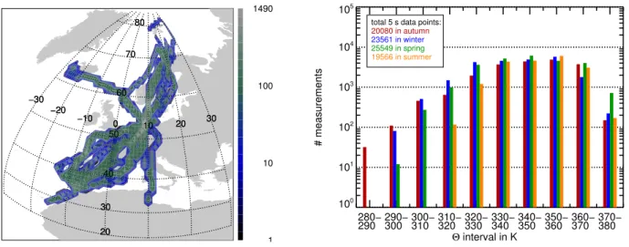
Figure 1 gives an impression of the obtained coverage of O3 (and H2O) measurements during SPURT in the ge-ographical and potential temperature space. The map in the left panel reflects the number of measurements in a 1◦longitude×1◦latitude bin. Each campaign consisted of a minimum of 2 flight days. On one day southbound and on the other day northbound flights were performed from and back to the Learjet basis Hohn (9.53◦E, 54.31◦N, northern Ger-many). The contours clearly accentuate the basis in north-ern Germany as well as the two main inter-stations, Faro in southern Portugal for the southbound flights and Tromsø in Norway for the northbound flights. Slow ascents and de-scents in these regions result in a large number of measure-ments there.
−30 −20
−10
0 10 20 30
20 30 40
50 60
70 80
−30 −20
−10
0 10 20 30
20 30 40
50 60
70 80
1 10 100 1490
280−
290 290−300 300−310 310−320 320−330 330−340 340−350 350−360 360−370 370−380 Θ interval in K
100 101 102 103 104 105
# measurements
total 5 s data points: 20080 in autumn 23561 in winter
25549 in spring
19566 in summer
Fig. 1. Distributions of obtained O3measurements during SPURT. Approximately the same distribution is valid for H2O (cf. Table A1 in
the Appendix). In the map (left), the number of 5 s data points in a 1◦longitude×1◦latitude grid is displayed. The colour bar reflects the number of data points in each geographical bin. The right chart shows frequency distributions of the same data in the potential temperature space, binned in 10 K steps. By this approach, a seasonal separation is performed (autumn, winter, spring, and summer, corresponding to red, blue, green, and orange, respectively). The total number of merged data points within the considered2range in each season is given in the upper left corner.
280 K and 310 K is a result of sampling, since the inlet of the FISH instrument was only opened at altitudes higher than a pressure value of≈400 hPa. Similarly, the JOE instrument provides high qualitative data at pressure altitudes above that pressure level (i.e.p<400 hPa). The frequency distributions in the2space reflect the SPURT concept of the flight pro-files. Slow ascents and descents allowed for accurately re-solved slant vertical profiles. Within each mission two flight legs at rather constant pressure altitude were performed, one near and the other above the tropopause (cf. numbers of data points within 320 K and 340 K and 350 K and 370 K, respec-tively). Due to fuel consumption and thus lower mass of the aircraft, at the end of each mission a climb to maximum al-titude (>370 K) was performed to sample generally undis-turbed stratospheric background air. The altitude flight pro-file was mirrored on the return flight to Hohn to sample the meteorological condition in two different height regimes.
To place the measurements in a meteorological con-text, ECMWF (European Centre for Medium-Range Weather Forecasts) analyses with a time resolution of 6 h interpolated to a 1◦×1◦grid in longitude and latitude on 21 pressure lev-els between 1000 and 1 hPa are used. Each analysis data set was further interpolated to 25 isentropic surfaces located be-tween 280 K and 400 K in steps of 5 K. On these isentropes potential vorticity (PV) is obtained by spatial and temporal interpolation to the flight tracks. The diagnosis of PV from meteorological data fields is affected by errors (e.g. Beek-mann et al., 1994; Good and Pyle, 2004). The procedure of data assimilation will remove obvious observational er-rors (Hollingsworth and L¨onneberg, 1989). The accuracy
in calculating PV is sensitive to the horizontal and vertical resolution and, in particular, small-scale meteorological fea-tures like tropopause folds are hardly represented in detail in the meteorological analyses. In contrast, in situ measure-ments have a much finer resolution and can therefore resolve small-scale features. This has to be considered when cor-relating model derived quantities with in situ measurements (cf. Sect. 4).
3 Seasonal cycles of O3and H2O in the UT and LMS
J
02 03F M 03A 02M J 03J 02A S 02O 01N D month and year
0 100 200 300 400 500 600 700 800
O3
in ppbv
1079 596 391 629 582 177 226 1097
1132684 691768 1388 15582070 1265 907 1308953 1429 321468 711407
2097 2321 1595 1811 1900 896 1702 1222
1229 934 1714 1929 1507 823 1654 1049
0− 1 PVU 2− 3 PVU
4− 5 PVU
6− 7 PVU 8− 9 PVU
max
min median
25 per 75
Fig. 2.Annual cycles of ozone mixing ratios in ppbv in the region of the UT and LMS as derived from the SPURT measurements. The observations are displayed as box plots in terms of potential vor-ticity, non-continuously incremented by 1 PVU due to facility of inspection (colour coding for 0–1, 2–3, 4–5, 6–7, 8–9 PVU), as in-dicated in the upper right corner. The median in each PV interval is represented by a dot, the box reflects the 25 and 75 percentiles, and the whiskers indicate minimum and maximum O3VMRs. Note the
month-year relation given by the labelling of the abscissa. The num-ber of data points considered in each box plot is given colour coded in the top row. The light and dark grey shadings display 3rd order polynomials fitted to the quartiles of O3data in the 0–1 PVU and
7–9 PVU range, to approximate the tropospheric and stratospheric seasonal cycles of O3as observed during SPURT, respectively.
3.1 O3in the UT and LMS
In Fig. 2 monthly median O3volume mixing ratios (VMRs) in different PV domains, characteristic for specific regions of the atmosphere, are shown as measured during SPURT. Thereby, a box plot graphing is used, showing centring (me-dian), spread (25 and 75 quartiles), and distribution (min-imum and max(min-imum). Despite the high information con-tent presented by the box plots, they can lead to misinterpre-tation or over-valuation of attributes in case of insufficient data. To provide an accurate impression of the central ten-dency and variability of O3 the number of considered data points in each box plot is additionally given in the top row, revealing that the considered amount of data in a PV domain should mainly be large enough to infer robust information from the box plots. Considering the complete data set, the seasonal variation of O3 in the UT shows a minimum dur-ing the winter and a broad maximum durdur-ing the sprdur-ing and summer measurements. This is highlighted by the light grey shading, representing 3rd order polynomial fits to the quar-tiles of O3measurements in the 0–1 PVU range.
There exists a number of regions showing a broad sum-mer maximum in tropospheric ozone. The existence of such a maximum is often associated with photochemical produc-tion (e.g. Logan, 1985). Thereby, O3 is formed by reac-tions involving volatile organic compounds and nitrogen ox-ide (NOx), driven by solar radiation. Many of these re-gions are continental and influenced by pollution (e.g. Lo-gan, 1989; Scheel et al., 1997). Also in the free tropo-sphere, a broad spring to summer maximum was observed (e.g. Logan, 1985; Schmitt and Volz-Thomas, 1997). Based on ozone sonde data from Observatoire de Haute-Provence (OHP) Beekmann et al. (1994) showed that the seasonal vari-ation of tropospheric O3is characterised by a large maximum during spring and summer. Furthermore, LIDAR and ozone sonde measurements from OHP from 1976 to 1995 give evi-dence for a shift from a spring maximum to a spring/summer maximum in the free troposphere (Ancellet and Beekmann, 1997). The observed broad spring/summer O3 maximum during SPURT in the UT with a slight shift towards spring is furthermore in accordance with results from Brunner et al. (2001).
Most variable O3VMRs were observed during the spring campaigns. During this season the influence of the large-scale downward motion is most prominent (Appenzeller et al., 1996). Also the net O3flux across the extra-tropical tropopause has a peak during spring to early summer, pri-marily affected by the outward O3flux of the LMS through the tropopause (Logan, 1999). Thus, the already enhanced tropospheric O3VMRs during spring seem to be effected by the downward transport of O3-rich stratospheric air during that season.
In PV domains >3 PVU, in the LMS, a clear maxi-mum during the spring and a minimaxi-mum around the autumn measurements is evident with a peak-to-peak amplitude of ≈400 ppbv O3within the PV range of 8–9 PVU. The quar-tiles of O3measurements in the 7–9 PVU range are fitted by 3rd order polynomials, assigned by the dark grey shading, to highlight the seasonal cycle of O3measured in the LMS. The ozone build-up in this atmospheric region occurs during winter as a consequence of poleward and downward trans-port, since the lifetime of O3is long with respect to chemical loss (e.g. Holton et al., 1995) and is largely controlled by dynamics (Logan, 1999). The observed spring maximum in the LMS over Europe during SPURT is most probably due to the downward advection of high O3VMRs by the strato-spheric winter/spring Brewer-Dobson circulation, in accor-dance with e.g. Logan (1985), Austin and Follows (1991), Oltmans and Levy II (1994), Haynes and Shepherd (2000), Prados et al. (2003). Ozone VMRs fall off from April/May to October with a strong average decrease rate in the 6– 9 PVU range of≈−78 ppbv/month. Much of this decrease is presumably caused by the change in tropopause height and transport mechanisms. On the basis of observations of SAGE II, Pan et al. (1997) and Wang et al. (1998) assumed that isentropic cross-tropopause inflow of tropospheric air into the LMS influences the seasonal cycle of O3(and H2O, see Sect. 3.2) in that atmospheric region, especially dur-ing summer. A maximum of quasi-isentropic inflow into the LMS during summer was also identified in model stud-ies by Chen (1995, 2-dimensional) and Eluszkiewicz (1996, 3-dimensional). Enhanced content of tropospheric air in September compared to May was identified by Ray et al. (1999) from balloon-borne chlorofluorocarbons and water vapour measurements, which was also thought to be owing to quasi-isentropic in-mixing of tropospheric air. The seasonal cycle of O3in the extra-tropics therefore differs between the UT and the LMS. The transition region between the UT and LMS (1–3 PVU) is rather influenced by the troposphere. Just above the tropopause layer (4–5 PVU) the stratospheric sig-nal becomes dominant.
Amplitudes of O3 VMRs grow with increasing PV. Re-garding the progression of O3VMRs through surfaces of in-creasing PV, the most prominent increase is apparent during winter and spring, whereas during summer and autumn the gradients are comparably weak. Since in Fig. 2 rather dy-namically similar air parcels are considered and PV exhibits a transport barrier, the lower O3gradients with respect to PV surfaces during summer and autumn suggest an intensified transport of tropospheric air into the LMS during these sea-sons (cf. Sect. 3.2). Towards higher PV ranges (>3 PVU), i.e. deeper in the LMS, tropospheric influence decreases which results in an increase in the slope (dO3/dPV). The ob-served variation of the slope has a maximum of about 60– 90 ppbv/PVU in April and a minimum of 10–30 ppbv/PVU in October. The results are comparable with findings from Beekmann et al. (1994) and Zahn et al. (2004).
3.2 H2O in the UT and LMS
As ozone, water vapour shows a distinct vertical gradient at the extra-tropical tropopause. Due to the temperature lapse rate and the decrease in pressure, water vapour VMRs de-crease exponentially with height from the troposphere up to the tropopause region. Calculated averages of measurements that span the transition region between the UT and the LMS are dominated by moist air from below the tropopause.
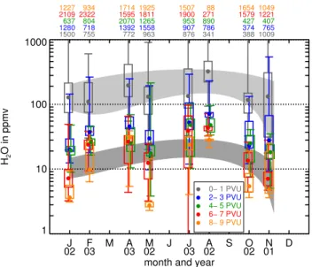
In Fig. 3 monthly values of H2O measured during SPURT are depicted in the same manner as for O3 (cf. Fig. 2). It is to note that the box plots in Figs. 2 and 3 are not dis-played chronologically in time (see labelling of abscissas). Based on the annual cycle of tropopause temperatures (e.g. Hoinka, 1999) and resulting ice saturation VMRs, maximum H2O VMRs in the tropopause region are expected during the summer, lowest during the winter months. In the PV range 0–1 PVU maximum H2O VMRs were measured dur-ing the campaign in August 2002. Alongside, the sprdur-ing campaign in April 2003 shows a second tropospheric max-imum, whereas during May 2002 and July 2003 comparably low H2O VMRs are apparent. This reflects the high variabil-ity of H2O in the probed atmospheric region, but is likely also sensitive to sampling (opening and closure altitude of the FISH inlet during ascents and descents). A tendency of higher VMRs during summer and lower ones during winter is present, which is evident from the accordant box plots in the 1–2 PVU (not shown) and 2–3 PVU range. As in Fig. 2, 3rd order polynomials are fitted to the measurements in the 0– 1 PVU range (light grey shading), to approximate the annual cycle of H2O in the UT. Across the tropopause the strong gradients in H2O are apparent. Considering northbound and southbound flights separately, the tropopause region at lower latitudes is slightly dryer than further north. This is probably due to the stronger influence of the dryer subtropical regions (see for instance Hoinka, 1999; Krebsbach, 2005).
J
02 03F M 03A 02M J 03J 02A S 02O 01N D month and year
1 10 100 1000
H2
O in ppmv
1500 755 772 963 876 341 388 1009
1280637 718804 1392 15582070 1265 907953 786890 374427 765407
2109 2322 1595 1811 1900 271 1579 1221
1227 934 1714 1925 1507 88 1654 1049
0− 1 PVU 2− 3 PVU
4− 5 PVU
6− 7 PVU 8− 9 PVU
Fig. 3.As Fig. 2, but for total water mixing ratios (in ppmv).
The measurements in February and April 2003 show higher H2O VMRs in the LMS than in May 2002, which probably indicates significant inter-annual variability but can also be influenced by sampling. The major part of flight legs during the southbound measurements in May 2002 were sit-uated in the vicinity of the tropopause. The meso-scale dy-namics indicates presence of subtropical air in the southern measurement region, i.e. lower in H2O and O3compared to mid and high latitude air (e.g. Hoinka, 1999; Krebsbach, 2005). In contrast, the aircraft extends deep into the strato-sphere on the northbound missions (cf. number of data in the 6–7 and 8–9 PVU ranges). This results in the established distribution of lower H2O VMRs in May compared to April 2003 in the 4–7 PVU range and thus largely affects the course of the approximated polynomials near MAM.
Air in the so called “overworld” (Hoskins, 1991) is de-hydrated as it is transported through the tropical cold trap. However, for a large extent of the performed SPURT cam-paigns H2O VMRs are considerably enhanced compared to stratospheric background values of about 2–6 ppmv (e.g. Hintsa et al., 1994). In the upper considered PV bins (>7 PVU) median values of observed H2O VMRs during the summer campaigns are about 20–30 ppmv and are moreover even measured in February and April 2003. These VMRs are much higher than could solely be explained by entry of air into the (lowermost) stratosphere in the tropics (e.g. Foot, 1984; Nedoluha et al., 2002). Values substantially larger than ≈6 ppmv are evidence for transport mechanisms of air into the LMS across the extra-tropical tropopause, and this signa-ture is carried deep into the lower stratospheric region.
Although there is no indication for a measurement arti-fact, the enhanced H2O VMRs observed in the LMS evoke consideration of instrument problems, e.g. cabin air leak, but which most likely can be excluded for several reasons. For instance, the campaign in February 2003 started with the
southbound flights where H2O VMRs of 20–30 ppmv con-comitant with 400–700 ppbv O3 were measured. On the northbound flights on the next day, H2O VMRs <6 ppmv were observed at O3VMRs of 600–750 ppbv, indicating that FISH was able to measure low stratospheric H2O VMRs, in particular, no changes were performed on the FISH in-strumentation during the whole campaign. The H2O VMRs measured during spring 2003 are also enhanced at PV levels above≈6 PVU. This campaign started on 27 April with the northbound flights where beside H2O VMRs<7 ppmv ex-ceptional enhanced H2O VMRs of about 20–35 ppmv were observed at O3 VMRs>600 ppbv. During the southbound flights, no such “abnormal” stratospheric conditions were en-countered. Fortunately, an added flight for inter-comparison of NOy instruments on the next day headed northward, al-lowing to measure once more in the region probed two days before. Again H2O VMRs of 25 ppmv concomitant with O3VMRs >600 ppbv were measured, which provides evi-dence for the correctness of data and debilitate instrument problems with leakage. Moreover, the SPURT flight con-cept, where most of the outbound flight legs were mirrored on the return flights to the campaign base, albeit at different altitudes, allows to cross-check the sampling on these south-bound and northsouth-bound flights. Thereby, the H2O distribu-tions are largely affirmed by both flights, suggesting robust-ness of the measured data.
Although enhanced H2O VMRs in the LMS are excep-tional, such conditions were encountered in all seasons dur-ing SPURT and thus seem not to be unlikely. Hegglin et al. (2004) discussed such an event probed during November 2001, and related it to the effect of recent convection with high reaching tropospheric injections during that time pe-riod. Also Tuck et al. (2003) reported about ER-2 flights near 60◦N in February 1989 with similar observations. Compara-ble high amounts of H2O accompanied with high O3VMRs were discussed recently by Dessler and Sherwood (2004) for the summer season and are also consistent with trace gas analyses by Ray et al. (2004b). Alongside, comparisons by G¨unther et al. (2004) of the SPURT observations with e.g. air mass spectra derived from model studies with the Chemi-cal Lagrangian Model of the Stratosphere demonstrate good agreement.
Another possible explanation for the encountered en-hanced H2O VMRs is provided by trajectory calculations. These occasionally suggest that air during troposphere-to-stratosphere transport processes is not generally freeze-dryed to its saturation value, by reason that e.g. the time for an ef-fective sedimentation and thus removal of ice water is too short. Saturation is rare in the LMS, allowing H2O-rich air to persist for a very long time period there. These aspects are currently investigated in more detail.
Combining the measurements of both campaigns in each season, the seasonal variability of H2O for observations in the tropopause region and in the LMS increases from SON/DJF towards JJA (see also Sect. 4). Note that the low variability of H2O in the PV bins above 6 PVU for the cam-paign in August 2002 is affected by the reduced amount of data, as mentioned earlier. The increase in variability to-wards summer suggests that the potential for transport of wa-ter through the tropopause is more effective and thus more important and significant during this season. This is espe-cially relevant for long-term transport which is the combined effect of mass transport and the efficiency of freeze-drying. Hence, as already derived from the O3data, the LMS seems to be more influenced by the troposphere during summer than during winter which is in agreement with the discussed sea-sonal variability of water vapour in the LMS by e.g. Pan et al. (2000).
Whereas the O3maximum measured in the UT is approx-imately in phase with the observed H2O maximum, it oc-curs about 2–3 months later (earlier) in the year as the O3 maximum (minimum) in the LMS. A similar time lag was found by Pan et al. (1997) and Prados et al. (2003). Due to the large debate, especially concerning the often observed spring O3maximum at some northern hemisphere stations, it is necessary to further investigate to what extent the corre-lation and/or anti-correcorre-lation of both trace gases could be at-tributed to dynamics or to chemistry. The seasonal cycles of O3and H2O obtained during the SPURT campaigns under-line the influence of two competing processes in the UT/LMS region: (i) subsidence of dry air from the overworld, which is primarily determined by the low tropical tropopause temper-atures and transported by the large-scale Brewer-Dobson cir-culation (e.g. Holton et al., 1995), and (ii) direct transport of moist air of tropical, subtropical or mid-latitude origin across the extra-tropical tropopause (e.g. Dessler et al., 1995; Hintsa et al., 1998). Whereas much of the air in the LMS has proba-bly been transported into the stratosphere by the former pro-cess, it is likely that local vertical transport processes play a much larger role in determining H2O in the UT/LMS. As is apparent in Fig. 3, in contrast to the O3VMRs, the observed seasonal cycles of H2O in the UT and LMS are roughly in phase with each other. This same seasonal course in both atmospheric compartments is a priori not clear, for instance due to integral effects. In particular, there is a strong decrease in H2O from August (maximum) where only measurements on southbound flights between 33–54◦N are available, to Oc-tober 2002. During August–OcOc-tober, the monsoons proba-bly enrich the LMS with tropospheric air. This air could be dryer than air transported into the LMS at mid-latitudes dur-ing summer and would thus lead to a relative strong decrease of H2O in the mid-latitude LMS. The observed lower H2O VMRs in October 2002 (and November 2001) thus suggests a significant contribution of upper tropospheric (sub)tropical air which previously has entered the LMS (cf. also results of Hoor et al., 2005; Hegglin et al., 2005).
4 O3and H2O in a view from different coordinates
The SPURT measurements covered a broad latitude range with different meteorological situations, often associated with small-scale phenomena (e.g. tropopause folds) and large-scale meridional advection of polar and/or subtropical and/or tropical air. The different dynamical impacts result in discontinuities and changes in the tropopause height, par-ticularly in the vicinity of regions with high wind velocities, the jet streams, in the literature often referred to as the region of the “tropopause break”. In order to get a comprehensive insight into distribution, spread, range, and variability of the measured trace gases in the SPURT region, 2-dimensional probability distribution functions (PDFs) are determined by using chemical, thermal, and dynamical vertical coordinates. Moreover, it is interesting to investigate which coordinate is best correlated with a trace gas and where the most compact correlation appears. An accurate correlation helps to deduce and to assess transport processes and provides the possibility for transformation into related quantities (see e.g. Krebsbach et al., 20061).
4.1 Probability distribution functions
In several SPURT flights, distinct cross-tropopause exchange events and characteristic features for specific meteorologi-cal situations could be identified. To obtain a compact view of the probed atmospheric region, PDFs are a tool to cen-tralise the large number of measurements. As an advantage of the PDFs, all measurement data is considered, and aver-aging is minimised. Thus, outliers become more visible and the prominent structures and features are revealed (Ray et al., 2004a).
In Fig. 4, PDFs of O3(left) and H2O (right) as a function of the thermal vertical coordinate potential temperature for the spring season are depicted. For the distributions obtained for the other seasons it is referred to Krebsbach (2005). Ozone is binned by 20 ppbv, H2O by 2 ppmv, and potential temper-ature by 5 K. The trace gas distributions are normalised to every bin of the thermal coordinate. This means, the colour coding reflects the probability in percent to measure a cer-tain trace gas VMR at a cercer-tain potential temperature. In addition, the mean and median value in each2bin is rep-resented by the solid and dashed coloured line, respectively. While the mean is an appropriate measure of the central ten-dency for roughly symmetric distributions, it is misleading when applied to skewed distributions since it can greatly be influenced by extremes. In contrast, the median is less sen-sitive to outliers and may be more informative and repre-sentative for skewed distributions. All seasonal means and medians are displayed to compare to each other (red, blue, 1Krebsbach, M., Schiller, C., Spelten, N., and G¨unther, G.:
280 300 320 340 360 380 Θ in K
0 200 400 600 800
O3
in ppbv
280 300 320 340 360 380
Θ in K 0
200 400 600 800
O3
in ppbv
MAM
280 300 320 340 360 380
Θ in K
0 50 100 150
H2
O in ppmv
280 300 320 340 360 380
Θ in K
0 50 100 150
H2
O in ppmv
0.3 1.0 3.0 10.0 30.0
Fig. 4.Seasonal 2-dimensional probability distribution functions of O3(left) and H2O (right) as a function of the thermal coordinate2for the spring measurements. The bin size is 20 ppbv for O3, 2 ppmv for H2O, and 5 K for2. The normalisation is performed to each2bin, i.e.
the probability (colour coding) reflects the percentage of an observed trace gas VMR in a single2interval. In both panels the mean and the median trace gas mixing ratios in each2interval are given by the solid and dashed lines, respectively, and are seasonally compared to each other (red, blue, green, orange corresponding to autumn, winter, spring, summer). In addition, the amount of seasonal data points considered in each2bin are presented in Table A1.
green, and orange for autumn, winter, spring, and summer, respectively). From a statistical perspective it is desirable to acquire as much information as possible. The chosen bin sizes of trace gases and the reference coordinate result from sensitivity studies of bin widths, in order to resolve specific characteristics and to reduce smoothing while considering an accurate amount of data in each grid box. The sensitivity studies were performed for each reference coordinate con-sidered in the following discussion. The seasonal number of data points in each2interval is displayed in Table A1 in the Appendix.
High probabilities, reflected by the light grey/green shad-ings, are very scattered throughout the O3distribution and, although both parameters, 2and O3, can be considered as vertical coordinates, no clear correlation is apparent. There is no symmetry around the mean or median values and mul-tiple modes can be noted. Generally, an increase of O3 VMRs with increasing2(height) is present, but the spread of O3VMRs on levels with constant potential temperature, the isentropes, is considerably large. The remarkable scatter and spread in the O3distributions is expected, since O3VMRs are largely dependent upon the location of the tropopause. The single flight missions extended over a large latitude range. Therefore, the variability of potential temperature at the tropopause location during each deployment along the flight path was sometimes quite large. For instance, on a flight from Hohn to Tromsø on 17 May 2002, the thermal tropopause (determined according to the WMO definition, WMO, 1986) was located at 304 K in the vicinity of Tromsø and at 328 K near the campaign base Hohn, which is a varia-tion of 24 K (see Krebsbach, 2005). However, also at higher isentropes, i.e. further away from the local tropopause, the spread in O3VMRs is considerably high.
The H2O PDF shown here as well as the distributions for the other seasons (see Krebsbach, 2005) exhibit similar characteristics as those for O3. The large variation of the tropopause location is apparent in the high amounts of H2O VMRs below≈340 K, with several local maxima and min-ima in the course of means (and partly of the medians) be-tween 300 and 320 K. A more compact distribution is only apparent above ≈340 K, with the higher variability during the summer season. Considering the largest seasonal dif-ferences of means and medians, i.e. between summer and winter, and shifting the mean H2O VMRs above≈330 K for the summer PDF by ≈20 K towards lower isentropes, the shape of the mean line (orange) is quite similar to the mean line for the winter season (blue). As illustrated by the num-ber of considered data points in Table A1, the SPURT mea-surements are mainly concentrated in the atmospheric region above isentropes of≈330 K. Strongest tropospheric influ-ence during summer, as already mentioned in the previous section, is thus in agreement with the seasonally integrated mass flux through troposphere-to-stratosphere transport by Sprenger and Wernli (2003, their Fig. 3b).
The shapes of the O3PDFs for the winter and spring mea-surements are quite different from the distributions obtained for summer and autumn (see Krebsbach, 2005). Whereas the former distributions show a more compact shape with a steady rise in O3VMRs with increasing2, the latter are less compact with a relatively weak and partly even no increase in O3 VMRs towards higher isentropes. This indicates an enhanced amount of air of recent tropospheric origin in the LMS compared to winter and spring. The large variabil-ity of trace gas VMRs, especially at higher isentropes (e.g.
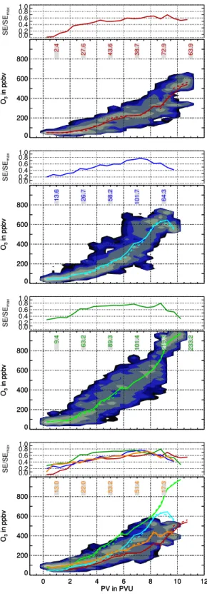
The picture drawn on the basis of2changes significantly when shifting the thermal coordinate to a dynamic coor-dinate, namely PV. The corresponding trace gas PDFs are shown for all seasons in Fig. 5 with PV incremented in 0.5 PVU steps. As is directly evident, O3is much stronger correlated with PV than with2, which is rather an accu-rate height or correlation parameter in the undisturbed strato-sphere. The range of O3VMRs on surfaces of PV is con-siderably suppressed when compared to the spread on isen-tropes and a general increase of O3with typically increasing height (PV) is now even apparent in the autumn and sum-mer distributions. The highest probabilities are mostly cen-tred in the distributions and symmetrically arranged around the mean or median O3 VMRs. In the PDFs, the slopes of the trace gas versus PV are calculated (see top numbers in Fig. 5). Hereby, a linear fit was performed within 2 PVU in-tervals to point out the essential character. The slopes are sig-nificantly stronger within 2–4 PVU than within the 0–2 PVU interval. The means and medians show commonly a change in increase in this range, indicating 2 PVU as a good proxy for the dynamically defined extra-tropical tropopause during the SPURT missions. Of course, the slope is weaker during summer, owing to the annual cycle of O3in the UT and in the LMS. The distinct seasonal cycles of O3in both atmospheric compartments, the UT and LMS, are clearly apparent in the PDFs.
For H2O, the spread in the PDFs is also reduced with PV as the reference coordinate. The sharp local minima and max-ima in the mean and median values in the2space (cf. Fig. 4 between 300 and 320 K), which are due to the varying lo-cation of the local tropopause, are significantly reduced or even absent when related to PV. Also above 2–3 PVU, i.e. within the tropopause region, the variation of H2O VMRs on PV surfaces is significantly reduced. However, during sum-mer the H2O derived distribution appears to be more compact when related to2. As is apparent from the structure as well as from the mean and medians, the seasonal cycles of H2O in the UT and LMS are reflected in the PDFs, with certainly higher VMRs measured during the summer campaigns in the UT and in the LMS.
The trace gas VMRs show a more compact distribution in a dynamical sense. In contrast to the spread and distribution of several high probabilities on isentropic surfaces, Fig. 5 re-veals that trace gas VMRs are more uniformly distributed and the probabilities vary less on PV surfaces. This indicates a more pronounced mixing state of trace gases on these sur-faces rather than on isentropic sursur-faces.
A further coordinate system to look at the trace gas dis-tributions and their variability is a coordinate system centred at the tropopause. Unfortunately, there was no instrument aboard the Learjet 35A measuring temperature profiles con-tinuously along the flight track from which the tropopause al-titude could be determined after the WMO definition (WMO, 1986). Nonetheless, as demonstrated earlier, the
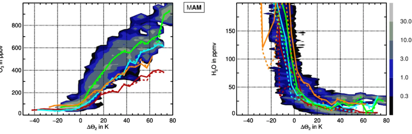
extra-tropical tropopause during SPURT can be derived dynami-cally from a PV threshold value, i.e. 2 PVU. The actual dis-tance in K of the aircraft’s location to the local dynamical tropopause (denoted as△2) is derived from the afore de-scribed ECMWF analyses by taking a certain PV surface as the extra-tropical tropopause. Note, the data resulting from processing of the ECMWF analyses (e.g. PV, △2) are not identical to the data presented in Hoor et al. (2004), where higher resolved T511L60 ECMWF data were used. Inter-comparisons for each campaign provide evidence for a clear agreement with correlation coefficients of>0.98 and slopes of 0.995 (±0.018). To account for the strong gradient of PV in the tropopause region, several PV threshold values were chosen as the dynamical extra-tropical tropopause, ranging from 2 to 6 PVU in 0.5 PVU steps. Through the different threshold values the character of the PDFs, i.e. location of high probabilities, spread and trace gas variability, does not change seriously. Thus, for representativeness, the O3 and H2O distribution related to the distance to the 2 PVU sur-face (△22) for the SPURT measurements during spring are shown in Fig. 6. For the distributions obtained during the other seasons as well as with△24as the reference coordi-nate it is referred to Krebsbach (2005).
The PDFs with respect to the distance to a threshold value of PV and the course of means and medians highlight the strong change in trace gas composition near 2 PVU. The dis-tributions are similar to those obtained in the PV space, al-beit the use of△2exhibits a slightly more compact shape, in particular for the campaigns in the winter and spring months (see also Sect. 4.3). The fact that the PDFs resemble in shape and distribution of probabilities in the view of PV and△2
suggests an advanced mixing state of these trace gases on surfaces aligned to the local tropopause. Each air parcel in the atmosphere can be thought of as being labelled by its PV, controlling or restraining the air parcels’ range of motion. A relatively huge degree of freedom is given in regions of uni-form PV (Sparling and Schoeberl, 1995). Thus, spatial gra-dients of PV might account for the dynamical affected trace gas distributions and not solely its absolute values. And this is exactly what the PDFs for different PV threshold values for the dynamically defined extra-tropical tropopause show, since the shape and the spread of distributions remain to the largest extent the same. This implies that the extra-tropical transition layer follows surfaces of PV or surfaces relative to the shape of the local tropopause, if defined by PV, rather than isentropic surfaces, in consistence with the results of Hoor et al. (2004).
4.2 Mixing entropy
0.0 0.2 0.4 0.6 0.8 1.0 SE/SE max 0 200 400 600 800 O3 in ppbv 0 200 400 600 800 O3 in ppbv
2.4 27.6 43.6 38.7 72.9 63.9
SON 0.0 0.2 0.4 0.6 0.8 1.0 SE/SE max 0 50 100 150 H2
O in ppmv
0 50 100 150
H2
O in ppmv
−161.5 −39.1 −5.0 −3.8 −2.0 −2.1
0.0 0.2 0.4 0.6 0.8 1.0 SE/SE max 0 200 400 600 800 O3 in ppbv 0 200 400 600 800 O3 in ppbv
13.6 26.7 58.2 101.7 64.3
DJF 0.0 0.2 0.4 0.6 0.8 1.0 SE/SE max 0 50 100 150 H2
O in ppmv
0 50 100 150
H2
O in ppmv
−123.3 −3.1 −5.1 1.3 8.8
0.0 0.2 0.4 0.6 0.8 1.0 SE/SE max 0 200 400 600 800 O3 in ppbv 0 200 400 600 800 O3 in ppbv
9.4 63.2 89.3 101.4 219.3 233.2
MAM 0.0 0.2 0.4 0.6 0.8 1.0 SE/SE max 0 50 100 150 H2
O in ppmv
0 50 100 150
H2
O in ppmv
−105.8 −12.2 −3.3 −1.7 13.1 −3.2
0.0 0.2 0.4 0.6 0.8 1.0 SE/SE max
0 2 4 6 8 10 12 PV in PVU
0 200 400 600 800 O3 in ppbv
0 2 4 6 8 10 12 PV in PVU
0 200 400 600 800 O3 in ppbv
13.0 22.0 53.2 51.4 17.3
JJA 0.0 0.2 0.4 0.6 0.8 1.0 SE/SE max
0 2 4 6 8 10 12
PV in PVU 0
50 100 150
H2
O in ppmv
0 2 4 6 8 10 12
PV in PVU 0
50 100 150
H2
O in ppmv
0.3 1.0 3.0 10.0 30.0
−154.5 −26.2 −3.1 −8.4 4.6
−40 −20 0 20 40 60 80
∆Θ2 in K
0 200 400 600 800
O3
in ppbv
−40 −20 0 20 40 60 80
∆Θ2 in K
0 200 400 600 800
O3
in ppbv
MAM
−40 −20 0 20 40 60 80
∆Θ2 in K
0 50 100 150
H2
O in ppmv
−40 −20 0 20 40 60 80
∆Θ2 in K
0 50 100 150
H2
O in ppmv
0.3 1.0 3.0 10.0 30.0
Fig. 6.As Fig. 4, but related to the distance to the local tropopause in K, considered as the 2 PVU surface. The bin size for△22is 5 K, the number of considered data points in each△22bin is given in Table A3.
respectively. Using these moments, the PDF is described by a relation to a single reference value, like the mean. This is probably inaccurate for a multi-modal distribution, where there is no symmetry around the reference (Sparling, 2000). A measure for the information content in a PDF for a trace gasµprovides Shannon’s entropy which is given as
SE= −
N
X
i=1
pi · ln pi (1)
(e.g. Srikanth et al., 2000), with ln as the natural logarithm. Concerning a PDF withDtotal observed data points of trace gasµandNbins of width△µ, the fraction of observation in theith cell (pi) is the number of observations within this cell
(Ni) divided byD, andPNi=1pi=1. The information content
is therefore solely dependent upon a given probability distri-bution and does not directly relate to the content or meaning of the underlying events, i.e. the quantity of the binned trace gas. Only the probability of the occurring events is impor-tant, not the events themselves. SE is zero if the distribu-tion has a maximum concentradistribu-tion, e.g. chemical homogene-ity within one bin. For a uniform spatial distribution, i.e.
pi=1/N ∀i, the considered trace gas field has a maximum
variability (any observed value can be placed in any one of theNbins) and the entropy is maximal (SE=SEmax=lnN). A maximum entropy implies indistinguishability of the air parcels. Moreover, they have an unrestricted free range of motion. In reality, PV constrains the air parcels’ range of motion. Thus, a maximum entropy value is not to be ex-pected (Sparling and Schoeberl, 1995). The maximum en-tropy is dependent upon the number of bins (see comment in Sect. 4.1). For a better comparison of different entropy val-ues, a normalisation to the maximum entropy is performed, resulting in
SE
SEmax
= −
N
X
i=1
pi · logN pi ≤1. (2)
The normalised mixing entropy is illustrated for O3and H2O with PV as the reference coordinate above each seasonal PDF in Fig. 5. In the O3 PDFs the normalised mixing entropy values enlarge with an increase in the coordinate value, i.e. height. Below PV values of ≈2 PVU the normalised mix-ing entropy is considerably small, indicatmix-ing only small-scale and low trace gas variability. A low mixing entropy value indicates a rather homogeneous air mass. This seems coun-terintuitive, since a well-mixed state, as an equilibrium state, should have maximum entropy. It should be noted thatSE
is distinct from the thermodynamical entropy. Thus, the en-tropy here is considered in the “chemical space” in contrast to the “physical space” (Sparling, 2000). The PDFs show high-est entropy values in the LMS for O3and in the troposphere as well as in the extra-tropical transition layer for H2O. The corresponding trace gas variability is maximal in these re-gions, implying the occurrence of different mixing states.
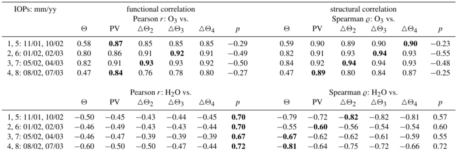
Table 1.Pearson’sr(left) and Spearman’s rank̺(right) correlation coefficients for O3(top) and H2O (bottom) versus potential temperature
(2), potential vorticity (PV), distance to the local dynamically defined tropopause (i.e. 2, 3, 4 PVU surface,△22,△23,△24, respectively),
and pressure (p). The coefficients of the eight single SPURT campaigns (IOP 1–8) are given for the two campaigns in each season, as indicated by the corresponding month and year (mm/yy). Best correlation coefficients (negative or positive) are highlighted in bold.
IOPs: mm/yy functional correlation structural correlation Pearsonr: O3vs. Spearman̺: O3vs.
2 PV △22 △23 △24 p 2 PV △22 △23 △24 p
1, 5: 11/01, 10/02 0.58 0.87 0.85 0.85 0.85 −0.29 0.59 0.90 0.89 0.90 0.90 −0.23 2, 6: 01/02, 02/03 0.80 0.86 0.91 0.92 0.91 −0.49 0.82 0.91 0.93 0.94 0.93 −0.55 3, 7: 05/02, 04/03 0.82 0.91 0.93 0.93 0.92 −0.50 0.84 0.92 0.94 0.94 0.93 −0.48 4, 8: 08/02, 07/03 0.47 0.84 0.76 0.78 0.80 −0.27 0.47 0.89 0.80 0.84 0.87 −0.25
Pearsonr: H2O vs. Spearman̺: H2O vs.
2 PV △22 △23 △24 p 2 PV △22 △23 △24 p
1, 5: 11/01, 10/02 −0.50 −0.45 −0.43 −0.44 −0.45 0.70 −0.79 −0.72 −0.82 −0.82 −0.81 0.57 2, 6: 01/02, 02/03 −0.46 −0.49 −0.43 −0.43 −0.44 0.70 −0.55 −0.60 −0.56 −0.54 −0.54 0.60 3, 7: 05/02, 04/03 −0.46 −0.47 −0.39 −0.39 −0.39 0.67 −0.67 −0.62 −0.62 −0.61 −0.59 0.55 4, 8: 08/02, 07/03 −0.60 −0.50 −0.50 −0.47 −0.44 0.72 −0.81 −0.64 −0.75 −0.72 −0.66 0.72
3 orders of magnitude, also for H2O above≈0–1 PVU. The strong increase inSE/SEmaxfrom 0–1 PVU for H2O is due to some data gaps in the selected bin widths and the result of the strong variation in H2O in the tropopause region with differentpis.
There are also strong gradients inSE/SEmaxfor H2O, e.g. near 8 PVU. They result (i) from the compact relationship between the trace gas and the reference coordinate in that re-gion (cf. PDFs) and/or (ii) from a bimodal distribution above ≈8 PVU, both decreasingSE/SEmax. During spring the O3 variability is highest in the LMS, probably due to the en-hanced downward motion. The O3entropy values are hence maximal during this season. The same arises for the en-hanced H2O content and its variability in the LMS during the summer months. Due to the most compact H2O PDF for the observations in autumn, the normalised mixing entropy values result in the lowest values in the range 6–8 PVU. The seasonal trace gas cycles are therefore reflected by the sea-sonal course of the mixing entropies.
Despite the comprehensive data coverage in the UT/LMS obtained during the SPURT project, it should be mentioned that to derive a more valuable statement from the mixing en-tropy, considerably more measurements are required, in par-ticular in the upper LMS.
4.3 Functional and structural correlations
A common measure for a relation between ordinal or contin-uous variables is the product-moment coefficient. Pearson’s correlation coefficient (r) reflects the degree of linear rela-tionship between two variables, sayx andy, of dimension
N. The functional correlation is defined as
rxy= N
P
i=1
(xi − ¯x)(yi− ¯y)
s
N
P
i=1
(xi− ¯x)2
s
N
P
i=1
(yi − ¯y)2
, (3)
withx¯ (y¯) as the mean of thexi’s (yi’s). It can range from
−1 to+1, inclusive, i.e. from a perfect negative to a per-fect positive correlation, wherebyr=0 indicates thatxandy
are uncorrelated. To decide, whether a correlation is signif-icantly stronger than another, Pearson’sr is not an accurate measure, since the individual distributions ofxandyare not considered.
A more structural measure for the relationship between two variables provides Spearman’s correlation coefficient (̺), which is a non-parametric or rank correlation. The com-putation is performed by replacing the value of eachxiby the
value of its rank, i.e. the smallest value of variablex is con-verted to rank 1, the highest to rankN. The same applies for theyi values. An outstanding advantage of the rank
correla-tion is that a non-parametric correlacorrela-tion is more robust than a linear correlation, in the same sense as the median is more robust than the mean (Press et al., 1997). After converting the numbers to ranks the Spearman correlation coefficient is calculated according to Eq. (3).
association between two parameters reveal the conclusion drawn from the PDFs. Trace gas isopleths of O3 seem to be orientated along surfaces of PV rather than along isen-tropes. The differences betweenrand̺for PV and the△2s are only small. In contrast, the correlations of O3with pres-sure are comparatively insignificant, nevertheless exhibiting larger structural negative coefficients during some winter and spring campaigns.
The correlation coefficients for H2O versus different pa-rameters are listed in Table 1 (bottom). When calculating Pearson’sr, H2O is best correlated with pressure. Both,p
and H2O, decrease very rapidly with height in a rather log-arithmic manner. Thus, the good correlation is to be ex-pected. This is especially evident during the summer cam-paigns (IOP 4 and IOP 8). Spearman’s̺is independent on the mode or shape of the distribution, and it renders unnec-essary to make assumptions on the functional relationship (Press et al., 1997). For this measure, H2O shows, as O3, a high degree of correlation when related to2,△2and PV.
5 Conclusions
The unique, continuous and high resolution O3 and H2O measurements, obtained during the SPURT campaigns be-tween November 2001 and July 2003, allow for a compre-hensive view of the UT/LMS region above Europe. In the first part, seasonal cycles of O3 and H2O in the UT and LMS have been analysed. As indicated by extensive stud-ies of vertical profiles obtained during ascents and descents (see Hoor et al., 2004; Krebsbach, 2005), the tropopause lo-cation, i.e. the noticeable boundary between the troposphere and the stratosphere, coincides well with the 2 PVU surface. Different analyses of the trace gas measurements reveal that the seasonal cycle of O3in the UT shows a spring to sum-mer maximum, most probably affected by in situ photochem-istry (cf. also Hegglin et al., 2005). In the LMS the sea-sonal O3cycle is more pronounced and shifted in phase by about 2–3 months earlier in the year, exhibiting a distinct spring time maximum. In the upper part of the LMS, a pro-nounced O3maximum is established during spring, whereas the lower part of the LMS still contains large contributions of rather O3-poor tropospheric air during winter and early spring. Only around April (2003) the O3maximum is also es-tablished in the lower part. This is the effect of the large-scale stratospheric winter/spring Brewer-Dobson circulation (see also Hegglin et al., 2005; Krebsbach et al., 2006). Induced by breaking Rossby waves and strong diabatic subsidence (the downward control principle, Haynes et al., 1991) aged and O3-rich stratospheric air is transported downward into the LMS (e.g. Austin and Follows, 1991; Beekmann et al., 1994; Logan, 1999). Thus, during spring a contribution of stratospheric O3due to stratosphere-to-troposphere transport is likely to affect tropospheric O3.
In contrast to the O3seasonal cycles, H2O shows no phase shift between the UT and the LMS. In a seasonal view, max-imum H2O VMRs were observed during the summer cam-paigns close to the tropopause in the UT as well as in the LMS. Lowest H2O VMRs were measured during the winter and autumn deployments, the latter indicating a temporally link with the subtropics/tropics (cf. Hoor et al., 2005, Heg-glin et al., 2005, Krebsbach et al., 2006b2). The reason for this seasonality is twofold. First, since H2O is strongly in-fluenced by heterogeneous processes, it follows the tempera-ture variation at the tropopause, i.e. the air is widely freeze-dried during its transport into the LMS (see also Krebsbach et al., 2006b). Second, whereas downward transport of dry air from the overworld into the LMS is dominant during win-ter, the barrier for quasi-isentropic transport of moist air over the tropopause deep into the LMS is weaker during summer. To examine the distribution, spread, and variability of both trace gases, especially 2-dimensional probability distribu-tions were used. Moreover, from these distribudistribu-tions, effects of transport and mixing processes can be inferred. Consid-ering several chemical, thermal, and dynamical coordinates, the measured trace gases are most compact arranged and best correlated when related to potential vorticity and to distance to the dynamically defined tropopause. Using various PV threshold values for the extra-tropical tropopause, the distri-butions show almost the same shape. The trace gas isopleths follow surfaces of PV or the shape of the tropopause, in ac-cordance with results from Hoor et al. (2004). This suggests an advanced mixing state in the LMS on surfaces relative to the shape of the tropopause.
The mixing entropy is assigned to characterise the PDFs and to estimate trace gas variability. Mixing entropy values for O3and H2O in the LMS appear to be maximal during spring and summer, respectively. This indicates highest vari-ability of these trace gases during the respective seasons with greater impact of stratospheric air during spring and tropo-spheric air during summer. Notwithstanding the extensive SPURT data set, still more data are necessary to derive more robust statements from the mixing entropy.
Despite the large seasonal and spatial data coverage, SPURT alone can obviously not provide a climatology but it reduces the lack of measurements in the UT/LMS, in par-ticular above Europe. The SPURT measurements can only provide instantaneous representations of the atmosphere en-countered during the single flights. To derive annual trace gas cycles, SPURT data from different years are assembled which are likely affected by inter-annual variability and/or by sampling. It must thus be emphasised that the results pre-sented here only apply for the SPURT region and have to be confirmed by further investigations and measurements.
2Krebsbach, M., Schiller, C., G¨unther, G., and Wernli, H.:
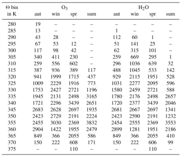
Table A1.Number of seasonal data points in each considered2bin in Fig. 4.
2bin O3 H2O
in K aut win spr sum aut win spr sum
280 19 – – – – – – –
285 13 – – – 1 – – –
290 43 28 – – 112 60 1 –
295 67 53 12 – 51 141 25 –
300 117 98 42 – 62 315 101 –
305 340 411 230 – 259 669 295 1 310 259 556 602 – 296 1036 639 32 315 387 936 389 117 488 1045 533 142 320 941 1999 1715 437 929 2115 1951 528 325 1009 2229 1916 773 1031 2277 2095 596 330 1753 2427 2721 1196 1580 2459 2721 588 335 1945 2131 2498 3165 1780 2176 2498 2657 340 1721 2296 3439 2651 1720 2377 3439 2046 345 2683 2628 2697 1935 2681 2667 2697 1341 350 2423 2729 2191 2224 2423 2590 2191 1232 355 2455 3030 2369 3832 2454 2555 2369 3553 360 2904 1422 1955 2479 2899 1281 1951 2186 365 849 366 2055 586 849 366 2055 410 370 150 222 608 171 150 222 606 99
375 – – 110 – – – 110 –
Table A2. Number of seasonal data points in each considered PV bin in Fig. 5.
PV bin O3 H2O
in PVU aut win spr sum aut win spr sum
0.0 327 855 544 198 348 1299 996 432 0.5 996 820 476 561 1049 956 739 785 1.0 1307 746 930 495 1420 961 927 408 1.5 1186 1187 975 823 1165 1298 988 730 2.0 643 1228 1559 844 652 1340 1563 488 2.5 389 595 1387 1371 487 658 1387 1205 3.0 703 620 832 862 690 703 832 684 3.5 573 683 1268 1399 558 741 1268 1177 4.0 467 512 1316 1180 449 562 1316 880 4.5 408 940 2019 1202 385 879 2019 963 5.0 428 1676 745 1277 416 1293 744 982 5.5 730 1362 1189 1087 694 1288 1189 800 6.0 954 1831 1587 1747 927 1827 1587 1437 6.5 1970 2587 1819 1049 1873 2604 1819 734 7.0 2119 3872 2416 1393 1858 3993 2416 833 7.5 2245 1628 2069 1454 2184 1533 2068 1089 8.0 1503 1510 2805 1920 1503 1508 2801 1378 8.5 1200 653 838 410 1200 653 838 217 9.0 871 183 446 251 871 183 446 173 9.5 225 70 214 42 223 70 214 16
10.0 426 – 110 – 423 – 110 –
10.5 378 – – – 378 – – –
Especially, the observed high amounts of H2O accompa-nied with stratospheric O3VMRs need further investigations and supporting model studies. Analyses of Arctic measure-ments near the northern SPURT area by Pfister et al. (2003) show no such occurrences. In contrast, these conditions have been encountered several times during SPURT, both on southbound and northbound flights, and it is not clear if these appearances can be attributed to climate trend or to geograph-ical conditions, e.g. wave breaking zone.
Table A3.Number of seasonal data points in each considered△22
bin in Fig. 6.
△22bin O3 H2O
in K aut win spr sum aut win spr sum
−45 3 – – – – – – –
−40 12 5 – – – – – –
−35 14 23 – – – – – 19
−30 14 35 – 66 26 – 2 78 −25 78 79 – 66 54 75 61 105 −20 162 155 26 131 173 208 152 194 −15 840 355 396 168 819 655 590 316 −10 825 1188 714 544 949 1483 996 669 −5 1969 1769 2077 1200 2059 2081 2138 1037
0 800 1767 2797 2218 845 1921 2800 1613 5 1023 1432 2278 1737 1027 1602 2278 1051 10 884 1220 3064 3713 837 1310 3064 3211 15 736 1185 1451 2260 695 1139 1451 1858 20 1188 2423 2391 2073 1091 1955 2391 1503 25 1968 1620 1973 1633 1715 1626 1972 967 30 1440 2142 796 1911 1377 2167 796 1475 35 1314 1165 1522 931 1313 1234 1522 811 40 839 1960 1997 241 839 1972 1994 179 45 1086 1391 968 164 1085 1334 968 80 50 1869 1014 772 151 1867 957 772 92 55 1214 1337 505 272 1212 1337 505 67 60 893 1044 636 86 893 1044 635 86
65 719 239 476 – 719 239 475 –
70 158 10 259 – 158 10 259 –
75 – – 384 – – – 384 –
Appendix: Number of data points considered in the PDFs
To provide an additional information for the robustness of the PDFs (Figs. 4–6), the number of data points considered in each bin of the reference coordinate are shown seasonally separated in Tables A1–A3.
Acknowledgements. SPURT is an AFO 2000 project and has been funded by the German BMBF (German: Bundesministerium f¨ur Bildung und Forschung) under contract No. 07ATF27 and addi-tionally supported by the SNF (Swiss National Fund). The authors acknowledge the ECMWF (European Centre for Medium-Range Weather Forecasts) for usage of meteorological data. We are also grateful to enviscope GmbH (Frankfurt a. M., Germany) for pro-fessional technical support and propro-fessional organisation. Further thanks are due to the pilots and the GFD (German: Gesellschaft f¨ur Flugzieldarstellung) for the excellent operation of the Learjet 35A.
Edited by: A. Stohl
References
Ancellet, G. and Beekmann, M.: Evidence for changes in the ozone concentrations in the free troposphere over southern France from 1976 to 1995, Atmos. Environ., 31, 2835–2851, 1997.
Appenzeller, C., Holton, J. H., and Rosenlof, K. H.: Seasonal vari-ation of mass transport across the tropopause, J. Geophys. Res., 101, 15 071–15 078, 1996.
Beekmann, M., Ancellet, G., and M´egie, G.: Climatology of tro-pospheric ozone in southern Europe and its relation to potential vorticity, J. Geophys. Res., 99, 12 841–12 853, 1994.
Brennikmeijer, C. A. M., Slemr, F., Koeppel, C., Scharffe, D. S., Pupek, M., Lelieveld, J., Crutzen, P., Zahn, A., Sprung, D., Fis-cher, H., Hermann, M., Reichelt, M., Heintzenberg, J., Schlager, H., Ziereis, H., Schumann, U., Dix, B., Platt, U., Ebinghaus, R., Martinsson, B., Ciais, P., Filippi, D., Leuenberger, M., Oram, D., Penkett, S., van Velthoven, P., and Waibel, A.: Analyzing At-mospheric Trace Gases and Aerosols Using Passenger Aircraft, EOS, 86, 2005.
Brunner, D., Staehelin, J., and Jeker, D.: Large-Scale Nitrogen Oxide Plumes in the Tropopause Region and Implications for Ozone, Science, 282, 1305–1309, 1998.
Brunner, D., Staehelin, J., Jeker, D., Wernli, H., and Schumann, U.: Nitrogen oxides and ozone in the tropopause region of the Northern Hemisphere: Measurements from commercial aircraft in 1995/1996 and 1997, J. Geophys. Res., 106, 27 673–27 699, 2001.
Chen, P.: Isentropic cross-tropopause mass exchange in the extrat-ropics, J. Geophys. Res., 100, 16 661–16 673, 1995.
Derwent, R. G., Simmonds, P. G., Seuring, S., and Dimmer, C.: Ob-servation and interpretation of the seasonal cycles in the surface concentrations of ozone and carbon monoxide at Mace Head, Ire-land from 1990 to 1994, Atmos. Environ., 32, 145–157, 1998. Dessler, A. E. and Sherwood, S. C.: Effect of convection on the
summertime extratropical lower stratosphere, J. Geophys. Res., 109, D23301, doi:10.1029/2004JD005209, 2004.
Dessler, A. E., Hintsa, E. J., Weinstock, E. M., Anderson, J. G., and Chan, K. R.: Mechanisms controlling water vapor in the lower stratosphere: “A tale of two stratospheres”, J. Geophys. Res., 100, 23 167–23 172, 1995.
Eluszkiewicz, J.: A three-dimensional view of the stratosphere-to-troposphere exchange in the GFDL SKYHI model, Geophys. Res. Lett., 23, 2489–2492, 1996.
Engel, A., B¨onisch, H., Brunner, D., Fischer, H., Franke, H., G¨unther, G., Gurk, C., Hegglin, M., Hoor, P., K¨onigstedt, R., Krebsbach, M., Maser, R., Parchatka, U., Peter, T., Schell, D., Schiller, C., Schmidt, U., Spelten, N., Szabo, T., Weers, U., Wernli, H., Wetter, T., and Wirth, V.: Highly resolved observa-tions of trace gases in the lowermost stratosphere and upper tro-posphere from the SPURT project: an overview, Atmos. Chem. Phys. Discuss., 5, 5081–5126, 2005,
SRef-ID: 1680-7375/acpd/2005-5-5081.
Foot, J. S.: Aircraft measurements of the humidity in the lower stratosphere from 1977 to 1980 between 45◦N and 65◦N, Quart. J. Roy. Meteor. Soc., 110, 303–319, 1984.
Good, P. and Pyle, J.: Refinements in the use of equivalent latitude for assimilating sporadic inhomogeneous stratospheric tracer ob-servations, 1: Detecting transport of Pinatubo aerosol across a strong vortex edge, Atmos. Chem. Phys., 4, 1823–1836, 2004, SRef-ID: 1680-7324/acp/2004-4-1823.
G¨unther, G., Schiller, C., Konopka, P., and Krebsbach, M.: Sim-ulation of Transport Processes in the Tropopause Region dur-ing SPURT usdur-ing a Lagrangian Model, Geophys. Res. Abstr., 6, 02609, 2004.
Haynes, P. and Shepherd, T.: Report on the SPARC Tropopause Workshop, Bad T¨olz, Germany, 17–21 April 2001, SPARC newsletter N. 17, 2000.
Haynes, P. H., Marks, C. J., McIntyre, M. E., Sheperd, T. G., and Shine, K. P.: On the “downward control” of extratropical diabatic circulations by eddy-induced mean zonal forces, J. Atmos. Sci., 48, 651–678, 1991.
Hegglin, M. I.: Airborne NOy-, NO- and O3-measurements
dur-ing SPURT: Implications for atmospheric transport, Ph.D. the-sis, Swiss Federal Institute of Technology Z¨urich, Diss. ETH No. 15553, 2004.
Hegglin, M. I., Brunner, D., Wernli, H., Schwierz, C., Martius, O., Hoor, P., Fischer, H., Parchatka, U., Spelten, N., Schiller, C., Krebsbach, M., , Weers, U., Staehelin, J., and Peter, Th.: Tracing troposphere-to-stratosphere transport above a mid-latitude deep convective system, Atmos. Chem. Phys., 4, 741–756, 2004, SRef-ID: 1680-7324/acp/2004-4-741.
Hegglin, M. I., Brunner, D., Peter, Th., Hoor, P., Fischer, H., Stae-helin, J., Krebsbach, M., Schiller, C., Parchatka, U., and Weers, U.: Measurements of NO, NOy, N2O, and O3during SPURT:
implications for transport and chemistry in the lowermost strato-sphere, Atmos. Chem. Phys. Discuss., 5, 8649–8688, 2005, SRef-ID: 1680-7375/acpd/2005-5-8649.
Hintsa, E. J., Weinstock, E. M., Dessler, A. E., Anderson, J. G., Loewenstein, M., and Podolske, J. R.: SPADE H2O
measure-ments and the seasonal cycle of stratospheric water vapor, Geo-phys. Res. Lett., 21, 2559–2562, 1994.
Hintsa, E. J., Boering, K. A., Weinstock, E. M., Anderson, J. G., Gary, B. L., Pfister, L., Daube, B. C., Wofsy, S. C., Loewenstein, M., Podolske, J. R., Margitan, J. J., and Bui, T. P.: Troposhere-to-stratosphere transport in the lowermost Troposhere-to-stratosphere from mea-surements of H2O, CO2, N2O and O3, Geophys. Res. Lett., 25,
2655–2658, 1998.
Hoinka, K. P.: Temperature, Humidity, and Wind at the Global Tropopause, Mon. Wea. Rev., 127, 2248–2265, 1999.
Hollingsworth, A. and L¨onneberg, P.: The verification of objective analyses: Diagnostics of analysis system performance, Met. At-mos. Phys., 40, 3–27, 1989.
Holton, J. R., Haynes, P. H., McIntyre, M. E., Douglass, A. R., Rood, R. B., and Pfister, L.: Stratosphere-troposphere exchange, Rev. Geophys., 33, 403–439, 1995.
Hoor, P., Gurk, C., Brunner, D., Hegglin, M. I., Wernli, H., and Fischer, H.: Seasonality and extent of extratropical TST derived from in-situ CO measurements during SPURT, Atmos. Chem. Phys., 4, 1427–1442, 2004,
SRef-ID: 1680-7324/acp/2004-4-1427.
Hoor, P., Fischer, H., and Lelieveld, J.: Tropical and extratrop-ical tropospheric air in the lowermost stratosphere over Eu-rope: A CO-based budget, Geophys. Res. Lett., 32, L07802, doi:10.1029/2004GL022018, 2005.
Hoskins, B. J.: Towards aP V −θview of the general circulation, Tellus, 43AB, 27–35, 1991.
Hoskins, B. J., McIntyre, M. E., and Robertson, A. W.: On the use and significance of isentropic potential vorticity maps, Quart. J. Roy. Meteor. Soc., 111, 877–946, 1985.
Hough, A. M.: Development of a two-dimensional global tropo-spheric model: Model chemistry, J. Geophys. Res., 96, 7325– 7362, 1991.