Seasonal observations of OH and HO₂ in the remote tropical marine boundary layer

www.atmos-chem-phys.net/12/2149/2012/ doi:10.5194/acp-12-2149-2012

© Author(s) 2012. CC Attribution 3.0 License.

Chemistry

and Physics

Seasonal observations of OH and HO

2

in the remote tropical marine

boundary layer

S. Vaughan1, T. Ingham1,2, L. K. Whalley1,2, D. Stone1,3, M. J. Evans3, K. A. Read4,5, J. D. Lee4,5, S. J. Moller2,3, L. J. Carpenter4, A. C. Lewis4,5, Z. L. Fleming6,7, and D. E. Heard1,2

1_{School of Chemistry, University of Leeds, Woodhouse Lane, Leeds, UK} 2_{National Centre for Atmospheric Science, University of Leeds, Leeds, UK}

3_{School of Earth and Environment, University of Leeds, Woodhouse Lane, Leeds, UK} 4_{Department of Chemistry, University of York, York, UK}

5_{National Centre for Atmospheric Science, University of York, York, UK} 6_{Department of Chemistry, University of Leicester, Leicester, UK}

7_{National Centre for Atmospheric Chemistry, University of Leicester, Leicester, UK} Correspondence to:D. E. Heard (d.e.heard@leeds.ac.uk)

Received: 23 June 2011 – Published in Atmos. Chem. Phys. Discuss.: 28 July 2011 Revised: 21 January 2012 – Accepted: 26 January 2012 – Published: 27 February 2012

Abstract. Field measurements of the hydroxyl radical, OH, are crucial for our understanding of tropospheric chemistry. However, observations of this key atmospheric species in the tropical marine boundary layer, where the warm, hu-mid conditions and high solar irradiance lend themselves favourably to production, are sparse. The Seasonal Oxidant Study at the Cape Verde Atmospheric Observatory in 2009 allowed, for the first time, seasonal measurements of both OH and HO2in a clean (i.e. low NOx), tropical marine en-vironment. It was found that concentrations of OH and HO2 were typically higher in the summer months (June, Septem-ber), with maximum daytime concentrations of ∼9×106 and 4×108molecule cm−3, respectively – almost double the values in winter (late February, early March). HO2was ob-served to persist at∼107molecule cm−3 through the night, but there was no strong evidence of nighttime OH, consis-tent with previous measurements at the site in 2007. HO2 was shown to have excellent correlations (R2_∼0.90) with both the photolysis rate of ozone,J(O1D), and the primary production rate of OH,P(OH), from the reaction of O(1D) with water vapour. The analogous relations of OH were not so strong (R2_∼0.6), but the coefficients of the linear corre-lation withJ(O1D) in this study were close to those yielded from previous works in this region, suggesting that the chem-ical regimes have similar impacts on the concentration of OH. Analysis of the variance of OH and HO2across the Sea-sonal Oxidant Study suggested that∼70 % of the total vari-ance could be explained by diurnal behaviour, with∼30 % of the total variance being due to changes in air mass.

1 Introduction

The hydroxyl radical, OH, is the dominant daytime oxidant in the troposphere. A major pathway for its formation is via the reactions

O3+hν(λ <340 nm)→O(1D)+O2 (R1)

O(1D)₊H2O→2OH (R2)

OH is closely coupled to the hydroperoxy radical, HO2, so that they are often referred to collectively as the family HOx (= OH + HO2). The key process for the formation of HO2in this region is the reaction

OH₊CO(₊O2)→HO2+CO2 (R3)

which is also one of the main loss processes for OH in a clean environment. In the absence of NO, OH can then be reformed from HO2via the reaction

HO2+O3→OH+2O2 (R4)

2

CH3O+O2→HO2+HCHO (R7)

In environments where the levels of NO are very low, the concentration of HO2is controlled by the loss processes

HO2+HO2→H2O2+O2 (R8)

HO2+CH3O2→CH3O2H+O2 (R9) HO2can also undergo heterogeneous loss with atmospheric aerosol, and this process has been shown to be important in the MBL (see, for example, Sommariva et al., 2004; Smith et al., 2006; Sommariva et al., 2006; Whalley et al., 2010). In environments with high concentrations of NO, the reactions

HO2+NO→OH+NO2 (R10)

RO2+NO→RO+NO2 (R11)

play an active role in the local chemistry. It is worth noting that the alkoxy radical, RO, generated in Reaction (R11) can react with O2to form HO2, as in Reaction (R7).

It has also been shown that the reaction of HO2with halo-gen oxides, XO (where X = Br, I)

HO2+XO→HOX+O2 (R12)

is significant in marine environments (Bloss et al., 2005b; Smith et al., 2006; Sommariva et al., 2006; Kanaya et al., 2007). The HOI and HOBr produced from Reaction (R12) can then either be removed through heterogeneous reaction with aerosol or photolysis to produce OH and a halogen atom, X. This halogen atom can then regenerate XO via the reaction

X+O3→XO+O2 (R13)

Read et al. (2008) and Mahajan et al. (2010) showed that the inclusion of the chemistry of halogen oxides, present at only a few pptv, was vital in order for model simulations to reproduce their observations of ozone – the key precursor for OH in the remote MBL – at the Cape Verde Atmospheric Observatory (CVAO) in 2007.

The rate of primary production of OH from Reactions (R1) and (R2) is given by

P (OH)₌2f_[O3] ×J (O1D) (1)

whereJ(O1D) is the photolysis rate of ozone and

f₌ kO1D+H2O[H2O] k_O1_D+H

2O[H2O] +kO1D+N2[N2] +kO1D+O2[O2] (2)

where the rate constants k_O1_D+H

2O (2.1 × 10− 10 _cm3 molecule−1 s−1), k_O1_D+N

2 (3.1× 10

−11 _cm3 _molecule−1 s−1_)andk

O1_D+O

2 (4.0 ×10−

11 _cm3 _molecule−1 _s−1_)are for the respective reaction and quenching processes of O(1D)

(Atkinson et al., 2004) atT _∼298 K, if all other removal pro-cesses for O(1D) are insignificant. The rate of production of OH, in the absence of NO, can thus be defined as

d[OH]

dt =P (OH)+k4[HO2][O3] + X

i

viJi[i]

−X

n

kOH+Ln[Ln][OH] (3)

wherei represents the other photolytic processes that may lead to generation of OH (vi is the stoichiometry of the pro-cess) and the last term is the total loss of OH to its sinks, such as the major reactions with CO and CH4and the mi-nor contributions from reactions with other VOCs, such as acetaldehyde. For remote environments containing low con-centrations of alkenes and other non-methane hydrocarbons, such as at the CVAO, the production of OH from the reaction of O(1D) with water vapour has been shown to dominate the production of OH. Using theMaster Chemical Mechanism, Whalley et al. (2010) performed a rate of production analysis for OH for this site and calculated thatP(OH) constitutes at least 75 % of the total rate of production of OH. Assuming that that the rate of OH production is dominated byP(OH) leads to the following steady-state expression:

[OH_{] =}PP (OH) n

kOH+n[n]=

P (OH)_×τOH (4)

whereτOHis the lifetime of OH with respect to its loss to all sinks. For a constant lifetime, a plot of [OH] againstP(OH) should be linear with slopeτOH. This equation can also be rewritten in terms ofJ(O1D) as

[OH] =(a_×J (O1D)b)₊c (5)

wherearepresents the influence of all chemical sources and sinks, b accounts for the effect of combining all photolytic processes that produce OH (i.e. photolysis of O3 as well as NO2, HOI, H2O2, etc.) into a single power function of J(O1D) (see Ehhalt and Rohrer, 2000), andcis the contribu-tion from all light-independent processes. Equacontribu-tions (4) and (5) have been used successfully to explain the variability of OH in different chemical schemes (e.g. Creasey et al., 2002, 2003; Berresheim et al., 2003; Smith et al., 2006).

In the absence of NO, the rate of production of HO2 is given by

d_[HO2]

dt =k3[OH][CO] −2k8[HO2] 2

−k_4[HO2][O3]

−k_9[HO2][CH3O2] (6)

As the rate of Reaction (R4) is slow compared to Reactions (R8) and (R9), and the rate of loss of CH3O2through reaction (R6) is slow compared to the rate of production, the steady-state concentration of HO2can be expressed as

[HO2]= s

k3_[CO][OH] 2k5+k7α =

s

k3_[CO] 2k5+k7α×

p

whereα= [CH3O2]/[HO2]. For constant values of [CO],α andτOH, a plot of [HO2] against√P (OH)should be linear.

As can be seen in Eqs. (1) and (2), the rate of production of OH is controlled by the concentration of water vapour and J(O1D). Thus, the high solar irradiance and the warm, hu-mid conditions in the tropics lend themselves favourably to OH generation. OH can then react rapidly with the many trace VOCs found in the troposphere, initiating their oxida-tion and, ultimately, the removal of these species from the atmosphere. This process is of particular importance when considering the role of OH in constraining the atmospheric budget of methane, the third most abundant greenhouse gas and second only to CO2of the long-lived greenhouse gases in terms of radiative forcing (Forster et al., 2007). Lawrence et al. (2001) used a global model to estimate that_∼75 % of atmospheric methane is oxidized between 30◦_{N and 30}◦_S. Bloss et al. (2005a) used the GEOS-CHEM model to esti-mate that 80 % of methane is removed in the tropical tropo-sphere through OH-initiated oxidation, with as much as 25 % of the total occurring in the MBL. Therefore, reliable mea-surements of OH in tropical areas are of crucial importance for understanding the global oxidizing capacity of the tropo-sphere and future climate change.

Simultaneous measurements of OH and HO2in the trop-ical boundary layer are still relatively sparse compared to the number of studies at mid-latitudes in the Northern Hemi-sphere, for example (see Heard and Pilling, 2003, and refer-ences therein). In recent years, the number of measurement campaigns in the tropics has increased, and Table 1 provides a brief summary of the results of previous studies in tropi-cal and remote MBL regions. Ground-based measurements of OH have been made at the Mauna Loa Observatory in Hawaii (Tanner and Eisele, 1995; Hoell et al., 1996; Eisele et al., 1996), although that station is∼3.5 km above sea level and, as such, the conditions are closer to free tropospheric than typical of the boundary layer. Airborne measurements of HOxwere made during the Pacific Exploratory Missions (PEM) (Hoell et al., 1999; Mauldin et al., 1999; Raper et al., 2001; Tan et al., 2001; Mauldin et al., 2001) and the Trans-port and Chemical Evolution over the Pacific (TRACE-P) campaign (Jacob et al., 2003; Mauldin et al., 2003; Cantrell et al., 2003; Olson et al., 2004), but measurements in the tropical boundary layer in both studies were limited. HOx -measurements have also been made over the tropical At-lantic Ocean and the pristine Amazon rainforests of Suri-name, Guyana and French Guiana (Lelieveld et al., 2008); on two separate campaigns in the Mexico City Metropolitan Area (Shirley et al., 2006; Dusanter et al., 2009a); at the Pearl River Delta, China (Hofzumahaus et al., 2009); over West-ern Africa as part of the African Monsoon Multidisciplinary Analyses (AMMA) campaign (Commane et al., 2010; Stone et al., 2010); and in Malaysian Borneo as part of the Oxidant and Particle Photochemical Processes (OP3) project (Hewitt et al., 2010; Pugh et al., 2010; Whalley et al., 2011; Stone et al., 2011a). However, these studies were predominantly in or

over either forested or polluted regions, so that the chemistry of HOxwas heavily influenced by processes other than Re-actions (R1)–(R12). There have been several studies in the remote MBL outside of the tropics – for example, at Cape Grim, Tasmania, as part of the Southern Ocean Photochem-istry Experiment (SOAPEX-2) (Creasey et al., 2003), and on remote Japanese islands (see Kanaya and Akimoto, 2002 and the references therein; Kanaya et al., 2007). However, measurements of OH and HO2in the remote tropical MBL are still very limited. Concentrations of OH were measured using Differential Optical Absorption Spectroscopy (DOAS) onboard the R/V Polarstern in the tropical Atlantic as part of the Air Chemistry and Lidar Studies of Tropospheric and Stratospheric Species on the Atlantic Ocean (ALBATROSS) project in late 1996 (Brauers et al., 2001). In that study, it was found that OH followed a clear diurnal cycle, with max-imum concentrations of about 7_×106molecule cm−3_at lo-cal noon, within the range observed above the tropilo-cal Pa-cific during the PEM. Also, [OH] and [HO2] was measured by Whalley et al. (2010) at the CVAO as part of the Re-active Halogens in the Marine Boundary Layer Experiment (RHaMBLe) in 2007 – the maximum daytime concentrations of OH and HO2 were 9×106 and 6×108molecule cm−3, respectively.

S.

V

aughan

e

t

al.:

Seasonal

obser

v

ations

of

OH

and

HO

Table 1.Summary of measurement campaigns of HOxin tropical and remote marine regions; studies that included measurements in the tropical MBL are shown in bold.

Campaign Location Environment Platform HOx Comments Reference

PEM-Tropics A

Pacific Ocean 30◦N–30◦S 75–165◦W

Marine Aircraft [OH]midday=6–8×106molecule

cm−3in boundary layer

Mainly higher altitudes (i.e. above 2 km). Dry season.

Hoell et al. (1999) Mauldin et al. (1999)

OKIPEX Oki Dogo Island, Japan 36.3◦N, 133.2◦E

Clean marine Ground HO2,peak∼9 pptv

HO2,night∼0–3 pptv

Good agreement between model and daytime HO2for some days, factor of 2 difference other

days.

Kanaya et al. (1999) Kanaya et al. (2000)

ALBATROSS Atlantic Ocean 5◦N–37◦S, 26–36◦W

Clean marine Ship up to [OH]∼107 molecule cm−3 in clean air

Model overpredicts OH by 16 % Brauers et al. (2001)

ORION99 Okinawa Island, Japan 26.9◦N, 128.3◦E

Clean marine Ground [OH]peak∼4×106molecule cm−3

HO2,peak∼17 pptv

HO2,night∼2–5 pptv

[HO2]:[OH]∼76; model underestimated

day-time HO2 by ∼20 % and cannot reproduce

nighttime HO2

Kanaya et al. (2001a) Kanaya et al. (2001b)

PEM-Tropics B

Pacific Ocean 36◦S–38◦N 76◦E–148◦W

Marine Aircraft [OH]midday=6–8×106molecule

cm−3in boundary layer (CIMS)

FAGE showed good agreement during inter-comparison flight.

Wet season.

Raper et al. (2001) Mauldin et al. (2001) Eisele et al. (2001) Aircraft OHmean∼0.1 pptv (<2 km)

HO2,mean∼10 pptv (<2 km)

Low altitudes – model overpredicts OH and HO2; HOxpredicted to be larger in spring

than autumn; OH seasonal changes due to changes in [O3], [H2O] andJ(O1D)

Tan et al. (2001) Davis et al. (2001) Olson et al. (2001)

RISOTTO 1999–2000

Rishiri Island, Japan 45.1◦N, 141.1◦E

Clean marine, semi-forested

Ground HO2,peak∼10 pptv

HO2,night∼0–8 pptv

Model underpredicts nighttime HO2and

over-predicts daytime HO2by∼70 %, but inclusion

of iodine chemistry improves agreement.

Kanaya et al. (2002a, b)

SOAPEX-2 Cape Grim, Tasmania 40.7◦S, 144.7◦E

Clean marine, semi-polluted and polluted

Ground [OH]peak=3.5×106molecule cm−3

[HO2]peak=2×108molecule cm−3

Good correlations between concentrations of both OH and HO2 with J(O1D), P(OH). Steady-state calculations overestimate [OH] in clean air by 20 %.

Creasey et al. (2003)

TRACE-P Pacific Ocean 14–33◦N 137.5◦E–146◦W

Marine Aircraft HO2up to 30 pptv (<1 km)

OH up to 0.4 pptv (<1 km)

HO2overpredicted and

OH underestimated at low altitudes. Dis-crepancy of∼50 % in intercomparison mea-surements of OH and HO2between two

in-struments on different aircraft.

Jacob et al. (2003) Mauldin et al. (2003) Cantrell et al. (2003) Eisele et al. (2003) Olson et al. (2004)

MCMA2003 Mexico City

19.4◦N, 99.1◦W (2.2 km altitude)

Urban polluted Ground [OH]peak=8–13×106molecule

cm−3

[HO2]peak=5–20×108molecule

cm−3

HO2,night=0.8–32 pptv

strong HOx scavenging during rush hour; τOH∼120 s−1; typical [HO2]:[OH]∼120;

val-ues of [OH] and [HO2] reported here have been

adjusted by factor of 1.6 from those reported in Shirley et al. (2006) as recommended by Mao et al. (2010)

Shirley et al. (2006)

Chem.

Ph

ys.,

12,

2149–

2172

,

2012

www

.atmos-chem-ph

ys.net/

V

aughan

et

al.:

Seasonal

obs

er

v

ations

of

OH

and

HO

2

2153

Table 1.Continued.

Campaign Location Environment Platform HOx Comments Reference

– Rishiri Island, Japan 45.1◦N, 141.1◦E

Clean marine, semi-forested

Ground [OH]peak∼2.7×106molecule cm−3 HO2,peak∼5.9 pptv

[OH]night=(0.7–5.5) ×106molecule cm−3 HO2,night∼0.5–4.9 pptv

Model overpredicts by 89 % and 35 % daytime HO2and OH, respectively.

Kanaya et al. (2007)

GABRIEL Amazon forest Atlantic Ocean 3–6◦N, 50–60◦W

Marine and forested

Aircraft [OH]mean,ocean=9.0×106 molecule cm−3

[OH]mean,forest=5.6×106 molecule cm−3

[HO2]mean,ocean=6.7×108 molecule cm−3

[HO2]mean,forest=10.5×108 molecule cm−3

Boundary layer concentrations; results sug-gest recycling of HOxover forest through ox-idation of isoprene

Lelieveld et al. (2008) Martinez et al. (2008)

MCMA2006 MILAGRO

Mexico City 19.4◦N, 99.1◦W (2.2 km altitude) (different site to MCMA2003)

Urban polluted Ground [OH]peak=2–15×106molecule cm−3

median [OH]peak∼5×106 molecule cm−3

[HO2]peak=0.6–6.5×108molecule cm−3

median [HO2]peak∼2×108 molecule cm−3

average diurnal HO2 peaks one hour after OH; [OH] correlates poorly withJ(O1D) and J(HONO); [HO2]:[OH] lower than in 2003; model underestimates both [OH] and [HO2]

Dusanter et al. (2009a, b)

INTEX-B Mexico City and Pacific Ocean 15–65◦N, 90–170◦W

Urban polluted and marine

Aircraft OHmedianup to 0.2 pptv (<2 km) HO2,medianup to∼15 pptv <(2 km)

Simultaneous with MILAGRO; levels of OH and HO2overpredicted by model below 2 km

Mao et al. (2009) Singh et al. (2009) Emmons et al. (2010)

PRiDE-PRD2006

Pearl River Delta, China

23.5◦N, 113.0◦E

Rural polluted Ground average diurnal peak values [OH]peak=13×106molecule cm−3 [HO2]peak=17×108molecule cm−3

Model severely underpredicts OH and HO2=> regeneration pathway independent of NO

Hofzumahaus et al. (2009)

AMMA West Africa 4–18◦N, 8◦W–4◦E

Marine and forested

Aircraft OH_∼0.2 pptv HO2∼15 pptv

Median mixing ratios at_≤0.5 km;

[HO2]:[OH]∼80; up to 10 pptv of HO2 ob-served at night; model gives good agreement for HO2 but overestimates OH by factor of 2.5

Commane et al. (2010) Stone et al. (2010)

RHaMBLe Cape Verde Atmo-spheric Observatory 16.9◦N, 24.8◦W

Remote marine

Ground [OH]peak=9×106molecule cm−3 [HO2]peak=6×108

molecule cm−3

HO2∼0.6 pptv measured on two nights

Good agreement with model predictions, es-pecially for OH; [HO2] strongly dependent on aerosol losses

Whalley et al. (2010)

.atmos-chem-ph

ys.net/12/

2149/2012/

Atmos.

Chem.

Ph

ys.,

12,

2149–

2172

,

2 T able 1. Continued. Campaign Loca tion En vironment Platform HO x Comments Reference OOMPH Atlantic Ocean 28–57 ◦ S, 46 ◦ W –34 ◦ E Remote marine Ship [OH] peak ∼ 6 × 10 6 molecule cm − 3 HO 2 , peak ∼ 15 pptv Good agreement with simple steady-state model for both species Hosaynali Be ygi et al. (2011) OP3 Danum V alle y, 5.0 ◦ N, 117.8 ◦ E (425 m a.s.l.) F orested Ground av erage diurnal peak v alue [OH] ∼ 2 × 10 6 molecule cm − 3 [OH] max =7.2 × 10 6 molecule cm − 3 Model o v erpredicts HO 2 and und erpredicts OH Whalle y et al. (2011) Malaysian Bor neo 4–7 ◦ N,114–120 ◦ E Marine and for ested Air craft [OH] mean =2.3 × 10 6 molecule cm − 3 [HO 2_] mean =3.3 × 10 8 molecule cm − 3 Boundary lay er ( < 2 km) Stone e t al. (2011) N AMBLEX Mace Head, Ireland 53.32 ◦ N, 9.90 ◦ W Remote marine Ground Range of noon-v alues [OH] max = 3–8 × 10 6 molecule cm − 3 [HO 2 ] max = 0.9–2.1 × 10 8 molecule cm − 3 Significant influence of halogen oxide chemistry on HO 2 concentrations Smith et al. (2011) Sommari v a et al. (2006) 2 Experimental

2.1 Measurement of OH and HO2radicals

HO2. Thus, there are typically 240 online and 60 offline one-second data points for HO2. The fluorescence signals are then normalised with respect to the laser power entering each detection cell (typically 10–30 mW in the OH cell, 3– 6 mW in the HO2cell).

The observed fluorescence signal,SOH(count s−1mW−1), were related to [OH] by

SOH₌COH_{× [}OH_] (8)

where COH is the sensitivity of the instrument (count s−1mW−1molecule−1cm3)with respect to OH and can be defined empirically by the expression

COH=D×TOH×fgate×8f (9)

whereD is a function of pressure-independent parameters (e.g. laser power, collection efficiency of the optics, quantum yield of detector),TOHis the transmission of OH within the instrument,fgateis the fraction of light sampled within the timing gate and8f is the fluorescence quantum yield from excited OH. The equations linkingSHO2, CHO2 and [HO2] are analogous to Eqs. (8)–(9). The sensitivity at a given cell pressure and water vapour concentration was calibrated by measuring the observed fluorescence of OH and HO2 gen-erated in a flow of air from the photolysis of a known con-centration of water vapour atλ= 184.9 nm (see Commane et al. (2010) for more details). Calibrations were performed regularly under the same conditions (i.e. laser power, instru-ment pressure) as for ambient sampling when possible and verified in the laboratory after the campaign.

The mixing ratio of ambient water vapour during the mea-surement periods (2–3 %) was greater than could be achieved in a field calibration (∼1.2 %). Hence, the calibrated sen-sitivities were corrected for the quenching of the OH fluo-rescence by water vapour using known rate parameters that contribute to the termsfgateand8f

fgate₌e−Ŵt1_−e−Ŵt2 ₍₁₀₎

8f₌τ −1

Ŵ (11)

where τ is the radiative lifetime of the excited OH state (A26+)in the absence of quenchers (688 ns; German, 1975), Ŵ is the total rate of removal of excited OH via radiative and quenching processes (calculated using the quenching rate constants of N2, O2 and water vapour at T ∼293 K reported in Bailey et al. (1997) and Bailey et al., 1999) andt1 andt2 are the start and cut-off times for the photon-sampling gates, respectively. By comparing the relative values of fgate and 8f for the conditions of the calibra-tion and atmospheric sampling, one can correct the sen-sitivity of the instrument to OH and HO2. These cor-rections lowered the instrument sensitivity by 10–30 %, raising the calculated [OH] and [HO2] by the same rela-tive proportion. The quenching-corrected instrument sen-sitivity (ct s−1mW−1molecule−1cm3) with respect to OH

was found to decrease through SOS, from _∼1.5_×10−7 _to ∼0.6_×10−7_{, possibly because of reduced transmission of} OH through the instrument or contamination/aging of the op-tics. The uncorrected sensitivity towards HO2 was gener-ally consistent at∼1.9×10−7ct s−1mW−1molecule−1cm3 throughout the campaigns, but increasing concentrations of water vapour from SOS1–3 led to effective instrument sen-sitivities (ct s−1mW−1molecule−1cm3)of ∼1.8×10−7 in SOS1 to ∼1.3×10−7 in SOS3. Recent work by Fuchs et al. (2011) has highlighted a possible interference to-wards HO2-detection by LIF from the chemical conversion of alkene- and aromatic-derived peroxy radicals to OH by NO which is added inside the fluorescence cell, with alkane-derived peroxy radicals exhibiting negligible interference. The concentrations of alkenes such as ethene and propene at the CVAO have been observed to be only a few pptv (see Car-penter et al. (2010) and Table 2). It is therefore expected that peroxy radicals derived from such alkenes generate only a very small HO2interference. Calculations using a box model incorporating the fullMaster Chemical Mechanismand con-strained using the VOC measurements at the site (Table 2) show that∼90 % of the RO2species are HO2 and CH3O2, with other significant species being CH3C(O)O2(5 %) and C2H5O2 (0.9 %), all of which showed no HO2interference during laboratory experiments. The RO2species OHC2H4O2 (0.6 % of RO2 total) and OHC3H6O2(0.6 %), derived from ethene and propene, respectively, do give some HO2 inter-ference (measured in the laboratory as 40 % with the exper-imental configuration used here), but their very low abun-dance leads to only a very small HO2interference. However, for other environments, such as forested or urban, where the concentrations of alkenes and aromatics may be considerably higher, HO2interferences from such RO2species may need to be taken into account.

The limits of detection (LOD) of OH and HO2, were de-fined as

LOD=S/N C_·P ·

s

1 m+

1 n

·σb (12)

2

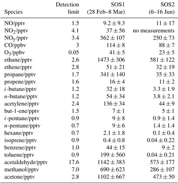
Table 2. Summary of the mean and standard deviations of NO,

NO2, NOy, CO, O3 and VOCs at the CVAO during the HOx

-measurement periods of SOS1 and 2. Note that the NO, NO2and

NOydata coverage was sporadic across these periods.

Detection SOS1 SOS2

Species limit (28 Feb–8 Mar) (6–16 Jun)

NO/pptv 1.5 9.2_±9.3 11_±17

NO2/pptv 4.1 37±56 no measurements

NOy/pptv 3.4 562±107 250±73

CO/ppbv 3 114±8 88±7

O3/ppbv 0.05 41±5 23±5

ethane/pptv 2.6 1473_±306 581_±122

ethene/pptv 2.8 51±21 32±19

propane/pptv 1.7 341±140 35±33

propene/pptv 1.6 16±4 11±2

i-butane/pptv 1.2 32±18 3.3±1.9

n-butane/pptv 1.2 54_±34 3.8_±2.1

acetylene/pptv 2.4 136±34 44±9

but-1-ene/pptv 1.5 7±1 5±1

i-pentane/pptv 0.9 9±8 0.9±1.4

n-pentane/pptv 0.7 9±6 1.4±1.4

hexane/pptv 0.7 2.1_±1.8 0.1_±0.4

isoprene/pptv 0.9 0.4±0.8 0.04±0.22

benzene/pptv 1.0 44±15 9±2

toluene/pptv 0.9 199±560 0.04±0.21

acetaldehyde/pptv 17.6 1142_±383 573_±177

methanol/pptv 7.0 690_±623 286_±107

acetone/pptv 2.8 1102±667 473±50

the square root of the sum of squares of the errors in the con-tributing variables, and was estimated to be∼32 % for both species.

The CVAO is located on the island of Sao Vicente (16.86◦N, 24.87◦W), approximately 10 m above sea level and about 50 m from the coastline; a full description of the site is given in Carpenter et al. (2010). Levels of NO are typically a few pptv (Lee et al., 2009), so the observatory is an ideal location for monitoring atmospheric composition in a clean, remote tropical MBL. The laser system and data-acquisition electronics were located inside an air-conditioned standard shipping container. The sampling inlet of the instru-ment was on the roof of this container inside an insulated alu-minium box, to protect against sea salt and water. To reduce the amount of scattered light detected, and also improve the transmission of OH and HO2through the instrument, a tube made of black nylon was placed inside the inlet between the sampling pinhole and the detection cell for OH, thus improv-ing both the sensitivity of the instrument and the limit of de-tection.

2.2 Ancillary measurements

The photolysis rate of ozone to produce O(1D),J(O1D), was measured using a 2π-filter radiometer mounted on the roof of the container, about 2 m from the FAGE inlet, and was

at no time in the shade of local influences (e.g. other instru-ments or structures at the CVAO). The signal from the ra-diometer was recorded as a voltage on the PC used to con-trol the FAGE instrument and was later converted to a pho-tolysis rate (s−1)using the parameters (including factors to correct for solar zenith angle, ozone column density and tem-perature) obtained during the intercomparison study in Julich (Bohn et al., 2008). These data showed almost 1:1 agreement (slope = 1.02;R2₌0.97) with the output of the University of Leicester’s spectral radiometer, which was positioned within a few metres at the same altitude, when the two radiometers were running simultaneously during SOS3.

Other ancillary measurements were made at the site, in-cluding those of NOx(i.e. NO and NO2), CO, O3, VOCs (in-cluding short-chain alkanes and alkenes, acetaldehyde, ace-tone, methanol), relative humidity and wind direction, to al-low characterisation of the atmospheric composition at the site. The majority of these measurements are part of a long-term dataset that has been running since 2006. Further de-tails of the relevant instrumentation can be found in Carpen-ter et al. (2010). Table 2 shows average measured values and standard deviations of important species for the periods with simultaneous measurements of OH and HO2 during SOS1 and 2.

2.3 Analysis of the data

The data were filtered for unfavourable meteorological con-ditions (e.g. heavy rainfall, as experienced during SOS3) and obvious influence of local pollution sources. Figure 1 shows examples of how pollution sources, such as the site power generator or passing fishing boats, distort the HO2:OH ra-tio on short timescales because of the conversion of HO2to OH by NO. Data were filtered out if the concurrent wind direction and speed data suggested that the sampled air mass was from an obviously polluted source, such as generator ex-haust fumes. The fast (i.e. 1 s) NOxdata would be required to allow identification of short pollution episodes from other sources, such as fishing boats; unfortunately, that data were not available for the bulk of the HOx-measurement period. The predominant wind direction was NE from the open At-lantic ocean (∼94 % of the time), with the generator located southerly to the HOx-instrument, so the wind direction (i.e. between 100◦ and 300◦) could be used to identify data af-fected by local pollution influences and then removed from the final analysis.

Fig. 1.[OH] (black) and [HO₂] (red) recorded at 1 Hz showing influences of pollution from passing boats on 16 June 2009 (left) and the site

power generator on 5 September 2009 (right); the green line in the left-hand panel is the 10 s running average of the OH data. The HO2data

in the right-hand panel have been offset by +2×108molecule cm−3for clarity.

Fig. 2. Plots showing two examples of measured HO2signals (black line) without(a)and with(b)significant variation in the laser

wave-length, observed as the response of the scaled reference cell signal (red line). The corrected HO₂-signals are represented by the green

lines.

power, instrument and reference cell pressures andJ(O1D) were constant (albeit for instrument noise) within each run and the early peaks in the reference signal correspond to where the laser wavelength was scanned to find the maxi-mum of the OH fluorescence. Figure 2a shows a run where the laser wavelength appears to be stable, as can be seen by the flat profile of the reference signal after_∼100 s. Fig-ure 2b clearly shows that the HO2signal appeared to follow the same pattern as the reference signal, such that the linear correlation between the two signals was reasonably strong (R2₌0.80). Because there was no evidence of significant changes inJ(O1D), laser power or the pressures inside the instrument and the reference cell, this effect was most likely as a result of small fluctuations in the laser wavelength. By normalising the OH- and HO2-signals to the reference sig-nal, one is able to correct for the small variations inλ, as can be seen by the green line in Fig. 2b. A similar correction ap-plied to the data in panel (a) suggested little change. Thus, this correction for small changes in wavelength, applied to the raw signals for both species, allowed data to be included in the analysis that may have otherwise been excluded.

3 Results

3.1 Summary of data and synoptic conditions

2

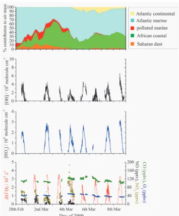
Fig. 3.Time-series of OH, HO₂and supporting measurements for SOS1. Top panel: source-region percentage contributions to air mass from Atlantic continental (yellow area), Atlantic marine (blue area), polluted marine (red area), African coastal (green area) and Saharan dust (brown area). Middle panels: observed concentrations

of OH (five-minute average) and HO2(four-minute average).

Bot-tom panel: five-minute averagedJ(O1D) (red line), and the average

mixing ratios of CO (green dots), O3(blue dots), NO (black dots)

and NO2(dark yellow dots); for clarity only the supporting data that

are simultaneous with HOx-measurements are shown.

noted that gaps in the time-series are either because the mea-suring instruments were not operational, the meteorological conditions were highly unfavourable during those times (e.g. heavy rainfall, very calm wind or strong wind from the direc-tion of local polludirec-tion sources), or the HOx-data failed cer-tain tolerances (e.g. laser instability, lack of NO flow). There were no measurements of NOxfrom 5–8 March, 11–16 June and no data for either NOx or CO for the whole of SOS3. It can be seen that HOxwas observed for 8, 11 and 14 days for SOS1, 2 and 3, respectively, and that both OH and HO2 followed clear diurnal cycles.

3.1.1 SOS1 (28 February–8 March 2009)

The conditions during the HOx-measurements for SOS1 (28 February–8 March) were warm (T _∼294 K) with very little rainfall. The average relative humidity was ∼77 %, corresponding to a concentration of water vapour of∼4.7×1017molecule cm−3. Winds were typically

north-Fig. 4. Time-series of OH, HO₂and supporting measurements for SOS2. Top panel: source-region percentage contributions to air mass from Atlantic continental (yellow area), Atlantic marine (blue area), polluted marine (red area), African coastal (green area) and Saharan dust (brown area). Middle panels: observed concentrations

of OH (five-minute average) and HO2(four-minute average).

Bot-tom panel: five-minute averagedJ(O1D) (red line), and the

aver-age mixing ratios of CO (green dots), O3(blue dots) and NO (black

dots); for clarity only the supporting data that are simultaneous with

HOx-measurements are shown.

Fig. 5.Time-series of OH, HO2and supporting measurements for SOS3. Top panel: source-region percentage contributions to air mass from Atlantic continental (yellow area), Atlantic marine (blue area), polluted marine (red area), African coastal (green area) and Saharan dust (brown area). Middle panels: observed concentrations

of OH (five-minute average) and HO2(four-minute average).

Bot-tom panel: five-minute averagedJ(O1D) (red line), and the average

mixing ratio of O3(blue dots); for clarity only the supporting data

that are simultaneous with HOx-measurements are shown.

Very few measurements of [HO2] were made on 6 March be-cause the supply for the injection of NO was closed to con-firm that the cylinder was not in any way a contaminating source of NO at the site.

3.1.2 SOS2 (6–16 June 2009)

The HOx-measurement period for SOS2 was characterised by warmer (T _∼297 K), with very few periods of cloud cover or rainfall. The mean relative humidity was_∼82 %, so that the average concentration of water vapour was ∼5.6_×1017molecule cm−3_{. As for SOS1, winds were} typ-ically north-easterly with speeds more than 4 m s−1_{. This} period experienced the cleanest conditions, with Atlantic marine air as the main source of the sampled air mass for the whole period, although coastal African air contributed up to ∼40 % on some days. There was little contribution from polluted marine air, Saharan dust or Atlantic continen-tal air. The noontime peak inJ(O1D) was quite consistent at∼3.7×10−5s−1for the whole period. CO and O3were

higher, at_∼100 and_∼30 ppbv, respectively, from 7–10 June compared to the rest of SOS2. These dates correspond to the highest peak [OH] and [HO2] for SOS2 of∼8×106and ∼4×108molecule cm−3, respectively. From 11 June to the end of SOS2, there was∼80 ppbv of CO and∼20 ppbv of ozone, and the daytime peak [OH] and [HO2] were rela-tively constant at∼5×106and∼2.7×108molecule cm−3, respectively.

3.1.3 SOS3 (1–15 September 2009)

2

and 3–4_×108molecule cm−3_{, respectively. The wind speed} dropped below 2 m s−1_{in the late afternoon of the 12th and} remained low through the 13th, similar to the conditions of the 5th, with the relative humidity rising to∼92 %. How-ever, there was no evidence of ambient HO2-OH conver-sion. Heavy rainfall again prevented measurements of OH and HO2on the 14th and most of the 15th.

3.2 Seasonal behaviour

Figure 6 shows the median half-hourly averaged diurnal pro-files of OH, HO2andP(OH) for SOS. The error bars repre-sent the 1σ day-to-day variability in the half-hour averaged data and, although the diurnal profiles for the three measure-ment periods do agree within the combined 1σ limits, the data around local noon (i.e. 10:00 to 14:00) for SOS1 is sta-tistically different (at 95 % confidence limit of a Student’s t-test) to the data in the same timeframe for both SOS2 and 3. The peak values of both [OH] and [HO2] followed the trend SOS1<SOS2∼SOS3, consistent with the trends in J(O1D) and water vapour concentration. Similar qualita-tive trends were observed for the sum of [HO2] and [RO2] recorded by the University of Leicester’s PERCA instrument (see Carpenter et al., 2010). However, P(OH) appears to fol-low the opposite trend (i.e. SOS1>SOS2∼SOS3) because the decrease in [O3] from SOS1 is larger than the combined increases inJ(O1D) and water vapour concentration. Possi-ble reasons for this discrepancy will be discussed in Sect. 4.1. The median ratio [HO2]/[OH] around local noon (10:00 to 14:00) was_∼75 for all three periods. During daylight, it may be expected for this ratio to vary inversely with [NO] because of conversion of HO2to OH via Reaction (R4). Simultane-ous coverage of [NO] (15 min averaging), [HO2] and [OH] was limited to only 22 % of the total HOxcoverage – 4 days in SOS1, 5 days in SOS2, with no NOx measurements in SOS3. Nevertheless, by taking half-hour averages of concur-rent [NO], [OH] and [HO2] between 08:00 and 17:00, it was found that [HO2]/[OH] was∼112 in air containing less than 5 pptv of NO and∼74 for greater than 5 pptv of NO. This trend is consistent with behaviour observed in other environ-ments (e.g. Carslaw et al., 2001; Creasey et al., 2002; Kanaya et al., 2001b), although it must be noted that the dataset in this case is limited to only 92 half-hour averages.

4 Discussion

4.1 Dependence of [OH] and [HO2] onJ(O1D) and

P(OH)

Figures 7 and 8 show [OH] and [HO2] as functions of J(O1D) andP(OH) for each of the three measurement pe-riods. Data from SOS1–3 are represented by black, red and green dots, respectively, and the blue lines represent the re-sults of the non-linear fits

Fig. 6. Half-hourly averaged median diurnal profiles of OH (top

panel), HO2 (middle panel) and primary production rate of OH,

P(OH) (bottom panel); SOS1–3 are represented by the black, red

and green lines, respectively. The error bars represent the 1σ

day-to-day variability of the data.

Fig. 7.Plots of five-minute averaged [OH] as a function ofJ(O1D)

(upper) andP(OH) (lower). Data from SOS1–3 are represented by

black, red and green squares, respectively, and the blue lines are the results of the non-linear fits to the complete datasets.

a change in the relative importance of HOx-sinks. It is worth noting that the values ofR2were virtually the same for the two types of fitting conditions. For ease of comparison with other studies, the following discussion will focus only on the results of the forced fits.

The results show that [HO2] has excellent correlations withpJ (O1_D)and√_{P (OH), for each measurement period} (R2₌0.88–0.95) and the whole SOS (R2₌0.88 and 0.87, respectively), suggesting that∼90 % of the variability of that species can be explained by a balance between its production from the reaction of OH and CO and its loss through self-reaction and self-reaction with CH3O2. These results also imply that the behaviour of HO2at the CVAO can be broadly de-scribed by the equations

Fig. 8. Plots of four-minute averaged [HO₂] as a function of

J(O1D) (upper) andP(OH) (lower). Data from SOS1–3 are

rep-resented by black, red and green squares, respectively, and the blue lines are the results of the non-linear fits to the complete datasets.

[HO2]/molecule cm−3=4.7×1010× q

J (O1_D)/s−1 ₍₁₄₎

[HO2]/molecule cm−3=1.2×105 ×

q

P (OH)/molecule cm−3s−1 ₍₁₅₎ A linear fit of [HO2] to √P (OH)τOH (see Eq. 7), where τOH is the lifetime of OH for each individual SOS cam-paign calculated from the linear fit of [OH] toP(OH), im-proves the correlation coefficient slightly (R2₌0.93). There is no further improvement in R2 when relating [HO2] to √

P (OH)τOH[CO].

2

Table 3.Results of the analytical fits of Eq. (13) forJ(O1D) to the observed five-minute averaged [OH] and four-minute averaged [HO2].

The units of a are molecule cm−3s (forb=1) and molecule cm−3s1/2(forb=0.5), for OH and HO2, respectively. The units ofcare

molecule cm−3. For ease of comparison, the values displayed in bold are those for forced fits ofb=1 andb=0.5 for [OH] and [HO2],

respectively; the values in parentheses are the results of unforced fits together with the standard errors onb. The values of R2 are virtually

the same for the respective forced and unforced fits.

OH HO2

a/1011 b c/106 R2 a/1010 b c/106 R2

SOS1 0.90 1(1.36±0.12) 0.39(0.46) 0.62 4.10 0.5(0.54±0.02) 5.6(10.6) 0.90

SOS2 1.09 1(0.71±0.08) 1.18(0.91) 0.56 4.76 0.5(0.42±0.02) 11.8(-3.8) 0.88

SOS3 1.30 1(0.91_±0.07) 0.25(0.17) 0.64 4.88 0.5(0.58_±0.02) ₋0.3(9.3) 0.90

All data 1.19 1(0.98±0.05) 0.48(0.50) 0.59 4.72 0.5(0.53±0.02) 3.4(7.5) 0.88

Table 4.Results of the analytical fits of Eq. (13) to the observed five-minute averaged [OH] and four-minute averaged [HO2] usingP(OH).

The units ofaares(forb₌1) and molecule1/2cm−3/2s1/2(forb₌0.5), for OH and HO₂, respectively. The units ofcare 106molecule

cm−3. For ease of comparison, the values displayed in bold are those for forced fits ofb=1 andb=0.5 for [OH] and [HO2], respectively;

the values in parentheses are the results of unforced fits together with the standard errors onb. The values ofR2are virtually the same for

the respective forced and unforced fits.

OH HO₂

a b c R2 a b c R2

SOS1 0.45 1(1.27_±0.13) 0.31(0.44) 0.59 0.91 0.5(0.55_±0.03) 5.6(10.6) 0.89

SOS2 0.82 1(0.89±0.07) 1.10(1.00) 0.68 1.30 0.5(0.47±0.02) 9.2(4.5) 0.95

SOS3 0.89 1(0.88_±0.08) 0.21(0.11) 0.64 1.29 0.5(0.57_±0.03) 1.1(9.7) 0.92

All data 0.70 1(0.79±0.05) 0.58(0.40) 0.53 1.18 0.5(0.48±0.02) 5.9(3.6) 0.87

can be slightly better described by a linear relation with J(O1D) (R2₌0.59) rather thanP(OH) (R2₌0.53). Sim-ilarly, averaging the data across longer time-periods only slightly improves the fit of Eq. (13) to the complete OH dataset. Also, the parametersa,b andcfor the raw 5-min data and the increased averaging agree within the standard errors of the fits; for example, two-hour averaging of the OH data results in fit parameters ofb₌0.94 (±0.14),c₌ 0.43 (±0.19)×106molecule cm−3andR2₌0.62, where the values in parentheses are the standard errors on the results of the fit. Thus, the fit results to [OH] suggest that 50–70 % of the variability of OH in each measurement period can be explained by the primary production process (R1–R2).

Comparing the three campaigns, the values ofa do not agree within the standard errors of the fits (for clarity, these are not shown in Tables 3 and 4) and follow the general trend SOS1<SOS2≤SOS3 for both OH and HO2, suggest-ing that the sources of HOxare greater and/or the sinks are less in the summer months than in winter. In fact,ais equal to the lifetime of OH for a linear fit of [OH] toP(OH). Thus, the results suggestτOH in the winter (∼0.45 s) is approxi-mately half that in the summer, implying that the sinks of OH

were stronger in SOS1 compared to SOS2 and 3. In terms of the relationship between HO2andP(OH) (Eq. 7) in a low-NOx environment, the parametera provides information of the mean ratio of [CH3O2] to [HO2],α, i.e.

aHO2−P (OH)= s

k_3[CO] 2k5+k7α×

√

τ (16)

Using average values of [CO] of 2.7 (SOS1) and 2.2 (SOS2) ×1012molecule cm−3 and the rate con-stantsk3= 2.3×10−13cm3molecule−1s−1,k5= 6.4 (SOS1) and 6.9 (SOS2)×10−12cm3molecule−1s−1 (the values are different because of the dependence of k5 on the concentration of water vapour and temperature) and k7= 5.3×10−12cm3molecule−1s−1, calculated using the recommendations in Atkinson et al. (2004) and Atkinson et al. (2006), provides values ofαof ∼4.1 and 2.1 for SOS1 and 2, respectively. These results suggest that HO2 could constitute up to 20 % of the total budget of peroxy radicals in winter compared to up to a third in the summer, if CH3O2is the dominant organic peroxy radical.

One possibility would be that the trend is a result of errors in the field calibrations – for example, the true sensitivity of the instrument for OH and HO2during SOS1 would have to be lower than that from derived from the calibration. The in-strument was calibrated by observing the signal from known concentrations of OH and HO2generated by the photolysis of water atλ= 184.9 nm using light from a mercury pen-ray lamp. An error or deviation in the calibration of the flux from that lamp would lead to a systematic error in the observed in-strument sensitivity. However, two different pen-ray lamps were used in the field, and the results of the instrument cal-ibrations were in good agreement. The field calcal-ibrations of the fluxes of these lamps at λ= 184.9 nm also agreed well with laboratory tests. These observations would suggest that the difference in the trends of [OH], [HO2] andP(OH) was not a result of errors in the instrument calibration.

The most likely explanation would be that there is season-ality in the sinks of HOx. Long-term measurements at the CVAO show that there is a tendency in the levels of VOCs to be higher in winter than in summer months, as shown in Table 2 (see also Read et al., 2009; Carpenter et al., 2010), which may explain, to some extent, the lower OH observed in February compared to June and September. However, one would still expect the reactions with methane and CO to be the dominant sinks for OH, and modelling studies suggest that CO represents 36.7 % and 38.1 % of the total OH loss during SOS1 and SOS2, respectively, while CH4represents 14.2 % and 18.0 % of the total OH loss during SOS1 and SOS2, respectively. It is known that the export of Saharan dust across the Atlantic Ocean exhibits strong seasonal be-haviour (see, for example, Schepanski et al., 2009). In win-ter, the dust layer is transported within the trade-wind layer in a south-west direction and at near-surface levels, frequently depositing in the region of the Cape Verde archipelago, while in the summer, the dust remains elevated above the boundary layer and is transported westwards (i.e. there is little deposi-tion to Cape Verde). Figures 3–5 show there was a small but significant contribution to the air mass from Saharan dust for SOS1 (up to∼15 %) and 3 (up to∼30 %), but little in SOS2. Also, aerosol sampling measurements at the CVAO revealed approximately half the samples were of high mass concen-tration (i.e. greater than 60 µg m−3) in the winter months compared to very few (∼5 %) in the summer months (see Carpenter et al., 2010). Whalley et al. (2010) used models to show that heterogeneous loss of HO2 on aerosols is an im-portant process in this region, constituting_∼23 % of the total loss of HO2 at noontime and leading to a reduction in day-time HO2of∼30 % compared to the modelled scenario with no aerosol uptake. Those authors also showed that the halo-gen oxides, IO and BrO, were important instantaneous sinks for HO2(∼19 %), despite being present at only a few pptv, and that the combined effects of heterogeneous losses and halogen oxide chemistry reduced modelled daytime HO2by ∼50 % compared to the modelled scenario without such pro-cesses; it should be noted, however, that the impact on OH

was only a few percent. It is conceivable, therefore, that the observed winter-summer trends observed in HO2in this study may be influenced by the seasonality of the concentra-tions of both aerosols and halogen oxides. Unfortunately, no measurements of halogen oxides were possible during SOS. The measurements by Mahajan et al. (2010) at the CVAO in 2007 suggested that the concentrations of both IO and BrO were relatively consistent throughout the year, although Whalley et al. (2010) suggested that the day-to-day variabil-ity in their measurements of OH and HO2could be explained by variability in concentrations of halogen oxides. A detailed modelling study is required to fully assess the chemical in-fluences on the seasonal behaviour of OH and HO2, and that will be the focus of a future paper.

4.2 Comparison with other measurements

2

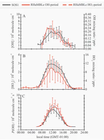
Fig. 9.Plots of the hourly-averaged median diurnal profiles of OH

(A), HO₂(B)andP(OH) (C)for SOS2 (June 2009; black lines)

and RHaMBLe (May–June 2007; solid red OH-measuring period,

dashed red HO2-measuring period). The error bars represent the 1σ

day-to-day variability in the hourly-averaged data. For clarity, the

error bars onP(OH) for the OH-measuring period are not shown.

It was found that the linear correlation between hourly-averaged values of [OH] and J(O1D) was poor in 2007 (a₌1.5×1011molecule cm−3s−1,c₌1.1×106molecule cm−3,R2₌0.35 forb set to 1; Furneaux, 2009), although it should be remembered that instrument difficulties led to only 5 days of OH measurements. No assessment of the relationship between [HO2] and J(O1D) or P(OH) was made. The ship-based measurements of [OH] over the trop-ical Atlantic ocean during ALBATROSS correlated quite well with J(O1D) (a₌1.4_×1011molecule cm−3s−1, c₌ 0.2×106molecule cm−3,R2₌0.72 forbfixed to 1; Brauers et al., 2001). The values of a from these two studies are close the average SOS value, suggesting that the effects of the chemical processing during the three different campaigns – separated by 13 yr – produced similar dependences of [OH] onJ(O1D). By taking an average of thea-values, the contri-bution to OH in the tropical Atlantic MBL from photolytic processes may be described by the expression

[OH_]/molecule cm−3₌1.3_×1011_×J (O1D)/s−1 (17)

However, the results shown in Table 3 suggest that there ap-pears to be a seasonal dependence of OH on J(O1D), so this expression should only be used as a crude approxima-tion when examining the long-term influence of OH in the tropical MBL.

4.3 Nighttime measurements of OH and HO2

Measurements of OH and HO2 at night (here defined as J(O1D)<10−7s−1, typically before 06:00 a.m. and after 06:00 p.m. local time) were limited, and a prolonged study of nighttime OH and HO2was only possible during one night of the SOS – 7 September 2009. The solid black lines in Fig. 10 represent the time-series of OH and HO2 for that night, the dashed line the respective LODs and the red line representsJ(O1D). It can be clearly seen that HO2persists into the night above the LOD, with an average concentra-tion of _∼107molecule cm−3_{. The values of [OH] for the} night of 7 September 2009 are normally distributed about ∼8_×104molecule cm−3_{, with a standard deviation close to} the five-minute LOD, suggesting that OH does not persist at measurable levels at least for that night.

Whalley et al. (2010) were not able to perform night-time measurements of OH at CVAO in 2007, so no comparison can be made. However, they did observe ∼107molecule cm−3of HO2at night, similar levels to those observed on the night of 7 September 2009. In fact, the mean concentration of HO2 when J(O1D)<10−7s−1 was ca. 107molecule cm−3 for SOS1–3, above the aver-aged LOD, suggesting that there was some persistence of HO2 at night in each of the three measurement periods. It is worth noting that 6(RO2+ HO2) was also observed to persist through the night at levels of almost 10 pptv (ca. 2.5_×108molecule cm−3_{)(see Carpenter et al., 2010).}

Whalley et al. (2010) observed that HO2 followed the nighttime profile of O3, suggesting that entrained air during the night was providing the source of radicals. On the night of 7 September 2009, O3remained constant at∼23 ppbv, so it was impossible to identify a link between [HO2] and ozone levels in this study. Whalley et al. (2010) also suggested that the source was the decomposition of peroxyacetyl ni-trate (PAN) and used a box model to show that∼100 pptv of PAN was sufficient to reproduce their nighttime levels of HO2. Nighttime levels of NOy, which would include PAN, of the order of hundreds of pptv were measured, so that pro-cess may have been an important source of nighttime HO2 during the SOS.

4.4 Seasonal variance analysis

Rohrer and Berresheim (2006) assessed which factors influ-enced the variability of OH over five years by calculating the contributions toVOH, the mean of the variances in [OH] divided into a range of timebins. For example, for a 5-yr dataset divided into timebins of 24 h,VOHwas calculated as the average of the daily variances of [OH]. Those authors then suggested that this total variance was a combination of three individual variances, such that

VOH₌(VOH_×R2(JO1D))₊Vinst₊Vother (18)

Fig. 10.The time-series of the five-minute averaged [OH] and

four-minute averaged [HO2] (solid black lines) and one-secondJ(O1D)

(red line) for the night of 7 September 2009; the dashed black lines

represents the five-minute and four-minute LODs (S/N=1) for OH

and HO2, respectively.

where the first term in this expression represents the mean variance of OH common toJ(O1D), whereR2(JO1D) is the square of the correlation coefficient for a power fit of [OH] to J(O1D) (i.e. Eq. 5),Vinstis the mean variance due to instru-ment noise, andVotheris the remaining variance due to other sources, including chemical influences. On subtractingVinst fromVOH, Rohrer and Berresheim found that the variance of OH across five years was dominated by the diurnal link to J(O1D) (76 %) and the seasonal cycle (23 %). It was shown that there was no observable long-term trend, such that there was a strong degree of seasonal stability in the relationship between [OH] andJ(O1D) across the five-year study. This behaviour suggested that competing chemical processes in-fluencing the fit parameters in Eq. (5) were compensating for each other across the seasons. This simple relationship was also shown to better describe the observed [OH] than a de-tailed chemical mechanism.

2

Fig. 11. The mean variances of 1 s(A), 30 s(B), 20 min(C)and one hour(D)averaged [OH] (left-hand panels) and [HO2] (right-hand panels) during SOS as a function of binsize; the different coloured lines correspond to the total variance (black), the variance due to instrument

noise (red), the variance due toJ(O1D)-dependence (blue) and the contribution from other sources (green). The dashed vertical black line

represents the timescale of individual measurement runs (i.e. five minutes).

the whole dataset was calculated. The difference between the mean total variance and the sum of the mean variances due to instrument noise and dependence onJ(O1D), is the variance due to unattributed sources, be that from factors influencing instrument noise not accounted for byVinstor chemistry con-trolling OH and HO2.

The results of the analysis are shown in Fig. 11. As would be expected, the influence ofJ(O1D) becomes more appar-ent at timebins where its value shows more variation (for in-stance, above 3 h). The variance of [OH] on a 1 s timescale is dominated by instrument noise (up to 75 % at 5-min binning), unsurprising given that the low concentration of this species leads to fluorescence signals just above the offline signal due

days. Nevertheless, the averaging has now made the tem-poral variability of [OH] across different timeframes more apparent; for instance, one can now clearly see that the vari-ance in [OH] across a day is a factor of∼3 more than across 5 min. Averaging across 20 min reduces the contribution of noise further, and it can be seen that the variances tend to more constant values with increasing time-averaging and that the variance of [OH] becomes more clearly controlled byJ(O1D).

The variance due to undefined sources,Vother, which in-cludes the variability in the chemical parameters control-ling OH and HO2 other than J(O1D), gradually increases with timebin-length for OH, but remains relatively constant for timebins greater than 6 days for HO2, suggesting that timescale as the order of which the air mass is changing. This result may not be unreasonable given the changes in O3, CO and air mass contribution observed during the SOS (see Figs. 3–5), and is particularly evident for SOS2. The day-to-day diurnal profiles ofJ(O1D) were very similar for this period. Figure 4 clearly shows that the levels of OH and HO2were relatively constant from 7–10 June, when the mix-ing ratios of CO and O3were also reasonably consistent at ∼100 ppbv and∼30 ppbv. The air mass was different for the remaining days of SOS2, with a smaller contribution from air originating from the African coast and lower levels of CO and O3, and the levels of OH and HO2are reduced compared to 7th–10th.

After subtracting the effects of instrument noise, the analy-sis suggests that_∼70 % of the variance of both OH and HO2 across the SOS can be explained by diurnal behaviour, and about 30 % from changing air mass and seasonal behaviour. It must be remembered that the SOS data are from three short, discrete periods, as opposed to the continuous 5-yr dataset of Rohrer and Berresheim. The sharp rises in vari-ances at the order of 2–3 days may be a result of using a non-continuous dataset containing measurements that were fre-quently only practical between 06:00 a.m. and 09:00 p.m. lo-cal time. Although not shown here, similar variance analysis within each of the three SOS measurement periods showed similar patterns as those seen in Fig. 11. Continuous, long-term measurements at the CVAO would provide better evi-dence of the existence of any genuine seasonal trends in [OH] and [HO2] and the relative contributions to the variance in those two species from diurnal and seasonal behaviour.

5 Conclusions

The Leeds aircraft-FAGE system, in its ground configuration, was successfully used to measure the concentrations of OH and HO2radicals at the Cape Verde Atmospheric Observa-tory for a total of 33 days over three periods of 2009 as part of the Seasonal Oxidant Study. This study was the first time that both OH and HO2have been measured in a tropical location in order to assess the seasonal variability of these species.

The concentrations of both OH and HO2followed the trend September_∼June>February–March, with maximum con-centrations of_∼9_×106and 4_×108molecule cm−3_, respec-tively, observed in the summer months, almost double the observations in winter, when increased levels of dust may act as an enhanced sink for HOx. The diurnal profiles of the June campaign agreed well with observations at the CVAO two years previously (Whalley et al., 2010). HO2was observed to persist into the night at levels of 107molecule cm−3, again consistent with the earlier work of The concentrations of both OH and HO2showed good correlations with J(O1D) andP(OH) were observed, particularly for HO2, with some differences in behaviour observed for summer and winter months. It was found that∼60 % and 90 % of the respective variabilities in observed OH and HO2, respectively, could be described by a simple steady-state approximation based on the primary production of OH from the photolysis of ozone and subsequent reaction of O(1D) with water vapour. The co-efficients yielded from a linear fit of [OH] toJ(O1D) are sim-ilar to those yielded from two previous studies in the tropical Atlantic MBL (Whalley et al., 2010; Brauers et al., 2001), possibly suggesting that the behaviour of OH in this region may be predicted using a simple expression. A variance anal-ysis of the data suggested that 30 % of the variance in [OH] and [HO2] across the study may be attributable to changes in the air mass, although it is recommended that a more com-plete dataset of observations would lend strength to this con-clusion.

The seasonal behaviour of OH observed in this study could have important implications for our understanding of the ox-idizing capacity of the Earth’s troposphere. However, the observed seasonal trend in OH observed during SOS does not fit with the simple chemistry scheme adopted here. A study of the ability of two atmospheric models to reproduce the observed behaviour in OH and HO2– and hence a test of the current understanding of tropospheric chemistry – is the subject of a future paper.

Appendix A

Methodology of variance analysis

2

900 one-second values for the 30 s, twenty minute and one hour averages, respectively (corresponding to 50 % of a full array for 30 s and 25 % for both 20 min and one hour aver-aging, a smaller fraction required for the latter two because these averaging times were longer than a typical run time, for which the instrument would only be online for 5 out of ∼8 min). The average values of each of those arrays was calculated and placed in a two-dimensional array that also contained the corresponding average Julian day for each ar-ray (ti)– for example, an hour is∼0.042 of a day, so that the corresponding array for the hourly-averaged OH data would begin

_t

i=1,ti=2,ti=3,...,ti=n [OH_]i=1,[OH]i=2,[OH]i=3,...,[OH]i=n

=

58.021,58.063,58.105,... [OH_]i=1,[OH]i=2,[OH]i=3,...

(A1) assuming that each of the original arrays contained sufficient one-second data to be included in the analysis.

The timebins that were chosen for the variance analysis were 5 min, 30 min, one hour, 11_{/2h, 2 h, 3 h, 4 h, 6 h,} 12 h, one day, 11_{/2days, 2 days, 3 days, 4 days, 6 days, 30} days and 200 days. These lengths of timebins were chosen to give the greatest spread in the variability ofJ(O1D) – and hence [OH] and [HO2] – within each timebin (i.e. very little across 5 and 30 min compared to across several hours and days). The timebin of 30 days was chosen so that the average variance would be the average of the variances of each of SOS1–3. The timebin of 200 days was used to calculate the variances across the whole of the SOS.

The variance analysis was carried out on each timebin length sequentially. Thus, the first variance analysis was per-formed using a timebin of five minutes. The campaign, start-ing at midnight 28 February 2009 and endstart-ing at midnight 16 September 2009, was divided into lengths of time equal to the value of the timebin. For example, there were approxi-mately 57 000 bins of five minutes. The variances of [OH] and [HO2],VOHandVHO2, within each timebin were calcu-lated by using the values of the appropriate array (A1) that fall within each timebin. Then, a non-linear fit of the equa-tion

[OH] =(a_×J (O1D)b)₊c (A2)

was made to the data in each timebin, and theR2value for that fit was multiplied by the value ofVOH orVHO2 for that timebin. Finally, the variance in [OH] or [HO2] due to instru-ment noise,Vinst, within each timebin was calculated using the following technique. The values of [OH] and [HO2] mea-sured at Cape Verde are calculated from

HOx(t )₌ Sig(t )

PD(t )_×C (A3)

where HOxrepresents either OH or HO2, not the sum of OH and HO2, Sig(t )is the raw HOxsignal (count s−1)at timet,

PD(t )is laser power (mW) andCis the instrument sensitivity (count s−1_mW−1_cm3_molecule−1_).V

inst, which is equal to σ2_HO

x, can thus be defined by _σ

HOx HOx

2 =_C12

_σSig Sig 2 + _σ PD PD 2

−2σSigσPD Sig×PDR

! (A4)

whereRis the correlation coefficient for a linear fit of PD(t ) to Sig(t ). The first (signal) term in the large parentheses represents the relative noise of the recorded fluorescence signal. The noise on the signal is defined as shot noise (i.e.σSig= Sig0.5), and the total raw signal before correction for background (i.e. total fluorescence + background counts per second) must be used. The second (PD) term in the large parentheses represents the relative noise of the recorded laser power (typically less than 5 %).Thus, Eq. (A4) simplifies to _σ

HOx HOx

2 =_C12

1 Sig+ _σ PD PD 2

−2σSigσPD Sig×PDR

!

(A5)

so that

V_inst=σ_HO2 x=

HOx 2

C2 × 1 Sig + σPD PD 2

−2σSigσPD Sig×PDR

! (A6)

Therefore, the contribution of instrument noise to the vari-ances in [OH] and [HO2] can be calculated from this equa-tion for each timebin. If the data are first averaged overx sec-onds, then the instrument noise is given by

σ_HO2 x=

1 x×

HOx 2

C2 × 1 Sig + _σ PD PD 2

−2σSigσPD Sig×PDR

! (A7)

Acknowledgements. The authors would like to thank A. Goddard, P. Edwards and staff in the mechanical and electrical workshops at the School of Chemistry, University of Leeds, for their technical assistance and logistical support throughout the course of this study. We thank R. Leigh of the University of Leicester for providing

J(O1D) data for comparisons of the two radiometers. We would

also like to thank B. Faria, L. Mendes and G. Duarte for their logistic assistance in Cape Verde. This project was funded by the NERC (NE/E011403/1), with support of the CVAO by the National Centre for Atmospheric Science (NCAS) and the SOLAS project.

Edited by: A. Hofzumahaus

References

Atkinson, R., Baulch, D. L., Cox, R. A., Crowley, J. N., Hamp-son, R. F., Hynes, R. G., Jenkin, M. E., Rossi, M. J., and Troe, J.: Evaluated kinetic and photochemical data for atmospheric

chem-istry: Volume I – gas phase reactions of Ox, HOx, NOxand SOx

species, Atmos. Chem. Phys., 4, 1461–1738, doi:10.5194/acp-4-1461-2004, 2004.