Modeling of 2008 Kasatochi volcanic sulfate direct radiative forcing: assimilation of OMI SO<sub>2</sub> plume height data and comparison with MODIS and CALIOP observations

(1)

www.atmos-chem-phys.net/13/1895/2013/ doi:10.5194/acp-13-1895-2013

Atmospheric

Chemistry

and Physics

Geoscientiic

Modeling of 2008 Kasatochi volcanic sulfate direct radiative forcing:

assimilation of OMI SO

2

plume height data and comparison with

MODIS and CALIOP observations

J. Wang1, S. Park1, J. Zeng1, C. Ge1,6, K. Yang2,4, S. Carn3, N. Krotkov4, and A. H. Omar5 1_{Department of Earth and Atmospheric Sciences, University of Nebraska, Lincoln, NE, USA} 2_{Department of Atmospheric and Oceanic Science, University of Maryland, College Park, MD, USA}

3_{Department of Geological and Mining Engineering and Sciences, Michigan Technological University, Houghton, MI, USA} 4_{Atmospheric Chemistry and Dynamics Laboratory, NASA Goddard Space Flight Center, Greenbelt, MD, USA}

5_{Science Directorate, NASA Langley Research Center, Hampton, VA, USA}

6_{State Key Laboratory of Atmospheric Boundary Layer Physics and Atmospheric Chemistry, Institute of Atmospheric}

Physics, Chinese Academy of Sciences, Beijing, China

Correspondence to:J. Wang (jwang7@unl.edu)

Received: 18 August 2012 – Published in Atmos. Chem. Phys. Discuss.: 5 October 2012 Revised: 29 January 2013 – Accepted: 4 February 2013 – Published: 19 February 2013

Abstract.Volcanic SO2column amount and injection height

retrieved from the Ozone Monitoring Instrument (OMI) with the Extended Iterative Spectral Fitting (EISF) technique are used to initialize a global chemistry transport model (GEOS-Chem) to simulate the atmospheric transport and lifecycle of volcanic SO2 and sulfate aerosol from the 2008 Kasatochi

eruption, and to subsequently estimate the direct shortwave, top-of-the-atmosphere radiative forcing of the volcanic sul-fate aerosol. Analysis shows that the integrated use of OMI SO2 plume height in GEOS-Chem yields: (a) good

agree-ment of the temporal evolution of 3-D volcanic sulfate dis-tributions between model simulations and satellite obser-vations from the Moderate Resolution Imaging Spectrora-diometer (MODIS) and Cloud-Aerosol Lidar with Orthog-onal Polarisation (CALIOP), and (b) an e-folding time for volcanic SO2that is consistent with OMI measurements,

re-flecting SO2oxidation in the upper troposphere and

strato-sphere is reliably represented in the model. However, a con-sistent (∼25 %) low bias is found in the GEOS-Chem sim-ulated SO2burden, and is likely due to a high (∼20 %) bias

of cloud liquid water amount (as compared to the MODIS cloud product) and the resultant stronger SO2 oxidation in

the GEOS meteorological data during the first week after eruption when part of SO2 underwent aqueous-phase

oxi-dation in clouds. Radiative transfer calculations show that

the forcing by Kasatochi volcanic sulfate aerosol becomes negligible 6 months after the eruption, but its global aver-age over the first month is −1.3 Wm−2, with the majority of the forcing-influenced region located north of 20◦N, and with daily peak values up to−2 Wm−2on days 16–17. Sen-sitivity experiments show that every 2 km decrease of SO2

injection height in the GEOS-Chem simulations will result in a∼25 % decrease in volcanic sulfate forcing; similar sen-sitivity but opposite sign also holds for a 0.03 µm increase of geometric radius of the volcanic aerosol particles. Both sen-sitivities highlight the need to characterize the SO2 plume

height and aerosol particle size from space. While more re-search efforts are warranted, this study is among the first to assimilate both satellite-based SO2plume height and amount

into a chemical transport model for an improved simulation of volcanic SO2and sulfate transport.

1 Introduction

(2)

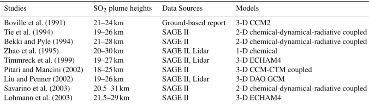
Table 1.Volcanic SO2plume modeling studies for the 1991 Pinatubo eruption.

Studies SO2plume heights Data Sources Models

Boville et al. (1991) 21–24 km Ground-based report 3-D CCM2

Tie et al. (1994) 19–26 km SAGE II 2-D chemical-dynamical-radiative coupled Bekki and Pyle (1994) 21–28 km SAGE II 2-D chemical-dynamical-radiative coupled Zhao et al. (1995) 20–30 km SAGE II, Lidar 1-D chemical

Timmreck et al. (1999) 19–27 km SAGE II, Lidar 3-D ECHAM4

Pitari and Mancini (2002) 18–25 km SAGE II 3-D CCM-CTM coupled Liu and Penner (2002) 19–26 km SAGE II, Lidar 3-D DAO GCM

Savarino et al. (2003) 20.5–31 km SAGE II 2-D chemical-dynamical-radiative coupled Lohmann et al. (2003) 21.5–29 km SAGE II 3-D ECHAM4

significant (Seinfeld and Pandis, 2006; IPCC, 2007; Wang et al., 2008). In contrast, stratospheric sulfate aerosols result-ing from volcanic eruptions can have lifetimes of 1–3 yr, and hence have more distinct but irregular (or sporadic) effects on global atmospheric chemistry and Earth’s radiative en-ergy budget (Budyko, 1977; Hofmann and Solomon, 1989; Deshler et al., 2006). Indeed, oxidation of volcanic SO2gas

by OH and H2O2 is a major pathway for producing

strato-spheric sulfate aerosols, which are highly scattering and in-crease planetary albedo in the UV and visible, and this in turn leads to radiative cooling of the Earth’s troposphere and surface (Robock, 2000). Through heterogeneous reac-tions, volcanic sulfate aerosols may also affect chlorine (such as ClO) and nitrogen (such as HNO3) chemical cycles in

the stratosphere, impacting ozone production and destruc-tion mechanisms (Hofmann and Solomon, 1989; Russell et al., 1996; Solomon, 1999). Solomon et al. (2011) showed that stratospheric aerosols have increased in abundance in the last decade, likely due to a series of moderate volcanic erup-tions (Vernier et al., 2011), resulting in a radiative forcing of

∼ −0.1 Wm−2_{in average, counteracting the positive forcing}

due to anthropogenic CO2.

Since the Nimbus 7 Total Ozone Mapping Spectrom-eter (TOMS) detected the SO2 clouds from the El

Chi-chon eruption in 1982 (Krueger, 1983), satellite measure-ments have been an indispensable tool for characterizing the spatio-temporal distribution of global volcanic SO2

emis-sions. These measurements use the strong SO2 absorption

band at 305–330 nm for retrieval of the total column amount of SO2. Carn et al. (2003) derived a long-term record of

vol-canic SO2 emissions from the TOMS satellites that were

in operation nearly continuously from 1978 to 2005. This data record is now being continued and improved with the OMI data (Levelt et al., 2006), and supplemented by so-lar backscatter ultraviolet (SBUV) measurements from the Global Ozone Monitoring Experiment (GOME) (Burrows et al., 1999) and GOME-2 (Munro et al., 2006), and by infrared (IR) measurements from the Moderate Resolution Imaging Spectroradiometer (MODIS) (Watson et al., 2004), Atmospheric Infrared Sounder (AIRS) (Prata and Bernardo, 2007), Infrared Atmospheric Sounding Interferometer (IASI)

(Karagulian et al., 2010) and Advanced Spaceborne Thermal Emission Spectrometer (ASTER) (Pieri and Abrams, 2010). However, while satellite-based SO2emission inventories

provide climate models with a unique description of the spatio-temporal distribution of volcanic SO2, they provide

limited information on the SO2 vertical distribution.

Con-sequently, current practice is to specify the SO2 injection

height using the volcanic explosivity index (VEI) of the erup-tion, which is assigned based on many observable parameters available from ground-based reports and is not necessarily an accurate indicator of volcanic SO2injection height (Spiro et

al., 1992; Simkin and Siebert, 1994; Andres and Kasgnoc, 1998; Robock, 2000). Indeed, in the TOMS SO2retrieval

al-gorithm, the SO2is assumed to be homogenously distributed

below either 5 km or 20 km altitude (Krueger et al., 1995, 2000). Hence, the lack of observation-based characterization of SO2plume height has led to various discrepancies in

quan-tification of the climatic effect of volcanic sulfate aerosols. As an example, Table 1 shows a list of different volcanic SO2

plume heights used in various modeling studies of the 1991 Pinatubo eruption; some studies derived the SO2 injection

height based on the same SAGE (The Stratospheric Aerosol and Gas Experiment) aerosol product, but obtain different es-timates. We note that volcanic sulfate aerosols are the result of oxidation of SO2, and hence, the difference in

gravita-tional settling velocity of SO2 gas and aerosol particles as

well as the vertical variation of atmospheric oxidation ca-pacity can yield discrepancies between the shapes of vertical profiles of volcanic aerosols and SO2plumes. Hence, while

aerosol vertical profiles can be a good proxy for SO2plume

injection heights, the direct retrieval of SO2 plume height

from satellite measurements is highly advantageous and is expected to improve modeling of the temporal variation and climatic effects of volcanic aerosols.

In recent years, new-generation satellite instruments such as the polar-orbiting hyperspectral UV sensors (e.g., OMI) and advances in retrieval techniques have expanded our abil-ity to measure volcanic emissions (Clarisse et al., 2008; Eck-hardt et al., 2008; Yang et al., 2009, 2010; Rix et al., 2012) beyond the total SO2 column amount. In particular, Yang

(3)

fitting (EISF) technique to simultaneously retrieve both SO2

amount and SO2 altitude from OMI measurements. They

found that EISF retrievals of SO2plume height were in good

agreement with other observations, and their estimate of SO2

amount has higher accuracy than those derived from the (op-erational) OMI linear fit retrieval algorithm (Yang et al., 2007).

To demonstrate the value of these advances in remote sens-ing of SO2 plumes for climate studies, in this paper we

use EISF SO2column and altitude retrievals (as in Yang et

al., 2009, 2010) to constrain a 3-D global chemical trans-port model (CTM; GEOS-Chem) simulation of the volcanic aerosol distribution and direct radiative forcing following the August 2008 eruption of Kasatochi (Aleutian Islands). Kravitz et al. (2010) illustrated the importance of 2008 Kasatochi volcanic aerosol forcing on a regional scale, al-though the climate effect on a global scale appeared insignif-icant; they assumed a total SO2 emission of 1.5 Tg which

was evenly distributed in three model layers (10–16 km) of a GCM. This study differs from prior modeling studies in that: (a) the CTM is initialized with the direct retrieval of the amount and injection altitude of volcanic SO2 from OMI,

(b) the CTM results are evaluated, and likely causes of un-certainties in the simulation of the volcanic SO2 lifecycle

from transport to sink terms in the atmosphere are diagnosed, with data from multiple A-Train satellite sensors including MODIS aerosol products, MODIS cloud products, additional OMI SO2data that are not used to initialize the CTM

simula-tion, and aerosol extinction profiles from the Cloud-Aerosol Lidar with Orthogonal Polarization (CALIOP), (c) a sensitiv-ity study is conducted to analyze the volcanic aerosol forcing as a function of SO2injection height specified in the CTM.

We describe the satellite data in Sect. 2, the configuration of the GEOS-Chem CTM and the method for calculating vol-canic aerosol radiative forcing in Sect. 3, present results of the baseline simulation in Sect. 4 and sensitivity simulations in Sect. 5, and finally summarize the paper in Sect. 6.

2 Satellite data

SO2data retrieved from OMI with the EISF algorithm (Yang

et al., 2009, 2010) are used in this study to initialize and validate the SO2distribution in the model. The EISF

tech-nique takes full advantage of the hyper-spectral BUV mea-surements from OMI to improve the accuracy of SO2column

retrievals and simultaneously determine the effective altitude of the SO2plume. It was designed to address the following

two disadvantages of earlier algorithms: (a) a priori assump-tion of the SO2vertical distribution that sometimes results in

large errors in the retrieved SO2amount; (b) underestimation

of SO2burdens, especially during large eruptions, because

the relationship between BUV radiance and atmospheric SO2

column increments is assumed to be linear whereas it actu-ally becomes non-linear as the SO2burden increases. In the

EISF algorithm, the SO2 vertical distribution is assumed to

be Quasi-Gaussian (with a fixed half width of 2 km in this study), and hence, the EISF retrievals provide an SO2amount

and effective plume altitude for each OMI footprint (24 km

×13 km at nadir).

The MODIS aerosol optical depth (AOD) product is used to validate our simulation of volcanic sulfate aerosol. The MODIS instruments aboard NASA’s Terra and Aqua satel-lites provide near daily global coverage at their local equato-rial overpass times of 10:30 a.m. and 1:30 p.m., respectively (Remer et al., 2005). Since MODIS AOD is a columnar quan-tity that has limited information about the aerosol chemical composition and aerosol vertical distribution, a direct com-parison between MODIS AOD and the modeled volcanic sulfate AOD is not straightforward, in particular when other types of aerosols dominate in the atmospheric column. How-ever, over remote regions where background AOD is gen-erally low, the spatial distribution of high MODIS AOD is still expected to be a good indicator of the transport path or distribution of volcanic aerosol. Hence, we use MODIS AOD for the evaluation of model-simulated transport pathways and distributions (instead of the absolute amount) of volcanic sul-fate aerosol. For this purpose, we use the MODIS level 3 AOD product (from both Terra and Aqua) with a spatial res-olution of 1◦×1◦and an uncertainty of±0.05 AOD±0.03 over the ocean and±0.20 AOD±0.05 over the land (Remer et al., 2005).

Since in-cloud oxidation is a major sink for volcanic SO2,

the MODIS(MOD08) level 3 cloud product (King et al., 2003) is used to evaluate the accuracy of cloud liquid wa-ter and cloud fraction in the GEOS-Chem model, which then provides a basis for the interpretation of any differences be-tween the GEOS-Chem simulated and OMI-observed SO2

(4)

the MODIS liquid water path data overall overestimates the counterpart retrieved from space-borne microwave (AMSR-E) instrument, although significant underestimation can also occur especially for broken clouds. While quantifying the un-certainties in MODIS liquid water path product in our study region and time period is challenging, all past studies sup-port that summation or averaging of MODIS liquid water path over a large spatial domain often reduce the uncertainty (Seethala and Horv´ath, 2010; Min et al., 2012), which is also the strategy used in this study during the intercomparison of MODIS and GEOS-5 liquid water path (Sect. 4.1).

To evaluate the model simulation of volcanic aerosols in the vertical direction, we compare model results with data from the Cloud-Aerosol Lidar with Orthogonal Polarization (CALIOP) instrument, aboard the Cloud-Aerosol Lidar and Infrared Pathfinder Satellite Observation (CALIPSO) satel-lite launched in 2006. CALIOP is a two-wavelength (532 and 1064 nm), polarization-sensitive (at 532 nm) lidar that measures atmospheric backscatter with a single-shot verti-cal and horizontal resolution of 30 m and 333 m, respectively. An extinction-to-backscatter ratio, also referred to as lidar ra-tio, is needed to convert the aerosol backscatter to extinction. The CALIPSO aerosol algorithm selects a “best-match” lidar ratio after a series of steps. (1) a cloud aerosol discrimina-tion (CAD, Liu et al. 2009) algorithm based upon probabil-ity distribution functions (PDFs) of layer averages of 532 nm backscatter, attenuated total color ratio, the midlayer altitude z, and the depolarization ratio is used to separate clouds from aerosols, and to differentiate layers of non-spherical dust par-ticles from layers of spherical parpar-ticles (e.g., liquid sulfate); (2) based upon the geolocation and season of CALIPSO ob-servations as well as the CAD in step (1), the aerosol type and the lidar ratio are selected from a look-up table that is gener-ated from cluster analysis of AERONET data and in situ ob-servations (Omar et al., 2005; Winker et al., 2009; Winker et al., 2010). To fulfill feature finding and layer classification re-quirements, the current CALIOP level-2 version 3 algorithm yields an aerosol profile product at a horizontal resolution of 5 km and vertical resolution of 60 m under 20 km altitude. In this study, the quality control flag in the CALIOP level-2 product is used to ensure high quality CALIOP retrievals of aerosol layers for comparing volcanic sulfate aerosols from the GEOS-Chem simulations.

3 Methodology

3.1 GEOS-Chem model, simulation initialization, and sensitivity experiments

A global 3-D CTM, GEOS-Chem (Bey et al., 2001), is used to simulate the evolution of volcanic SO2. The model is

driven by assimilated meteorological data from the GEOS at the NASA Global Modeling and Assimilation Office (GMAO). In this study, version 9-01-01 (http://GEOS-Chem.

org) is used at 2◦_×_2.5◦_{resolution with GEOS-5 47-level} 3-hourly meteorological fields (interpolated at every 15 min-utes to match the time step in the GEOS-Chem). Convective transport in the model is calculated from the convective mass fluxes in GEOS-5 meteorological fields (Wu et al., 2007). For boundary layer mixing the non-local scheme is used (Lin and McElroy, 2010). The wet deposition schemes for water-soluble aerosols (Liu et al., 2001) and for gases (Mari et al., 2000) are implemented. Dry deposition is based on the resistance-in-series scheme (Wesely, 1989), with the consid-eration of the hygroscopic growth of aerosol particles (Park et al., 2004). Anthropogenic emissions of SO2in the model

use as default the EDGAR 3.2 global inventory for 2000 (Olivier and Berdowski, 2001). The model also uses global biofuel emissions (Yevich and Logan, 2003), anthropogenic emissions for black carbon and organic carbon (Bond et al., 2007), shipping emissions from ICOADS (Lee et al., 2011), biomass burning from the GFED-2 inventory (van der Werf et al., 2009), and a lightning NOxemissions algorithm (Price

and Rind, 1992). Eruptive and non-eruptive volcanic SO2

emissions for each year are implemented in the model using the AEROCOM hindcast emission data (Fisher et al., 2011), but for the Kasatochi volcanic emissions, we use the OMI EISF data (see description below). The default eruptive vol-canic SO2data provide daily emissions that are on a generic

1◦×1◦ grid and are re-gridded into 2◦×2.5◦resolution in the model.

Aerosol simulation in GEOS-Chem includes the sulfate-nitrate-ammonium system (Park et al., 2004), carbonaceous aerosols (Park et al., 2003), sea-salt (Alexander et al., 2005), and mineral dust (Fairlie et al., 2007), and couples with gas-phase chemistry (Jacob, 2000) through nitrate and am-monium partitioning (Park et al., 2004), sulfur chemistry (Chin et al., 1996; Alexander et al., 2009), secondary or-ganic aerosol formation (Fu et al., 2008), and uptake of acidic gases by sea salt and dust (Evans and Jacob, 2005; Fairlie et al., 2010). GEOS-Chem includes all major sink terms for SO2 in the atmosphere, including oxidation by

the hydroxyl radical (OH) in the gas phase and by ozone (O3) and hydrogen peroxide (H2O2) in the aqueous phase

at temperatures above 258 K (Fisher et al., 2011; Wang et al., 2008a). Stratospheric chemistry in GEOS-Chem is based on climatological representation of species sources and sinks, and uses the Linoz algorithm of McLinden et al. (2000) to simulate stratospheric O3 (http://wiki.seas.harvard.edu/

geos-chem/index.php/Stratospheric chemistry). The sulfate aerosols are partly or totally neutralized by ammonia (NH3),

(5)

those from ground-based observations (Park et al., 2004; Martin et al., 2004).

The current simulation of the evolution of volcanic SO2

emitted by the Kasatochi eruption was initialized with the spatial distribution of OMI EISF SO2amount (Fig. 1a) and

effect height (Fig. 1b) on 8 August 2008. SO2plumes with

column amounts up to 250 DU and effective altitudes up to 10 km can be seen around 52◦N, 165◦E (Fig. 1a and b). Blocked by a ridge with center line along 155◦W (Fig. 1c), the plume was unable to move eastwards, but instead circu-lated around a low pressure system (centered around 50◦N, 170◦W) following the anti-clockwise cyclonic flow, and hence quickly diluted westwards, to 50 DU with an effec-tive height of 4–6 km in the downwind region around 50◦N, 172◦_{W (Fig. 1a and b). Based upon the distribution of the} SO2amount and effective altitude respectively in Fig. 1a and

b, the vertical distribution of SO2(as a function of altitude)

is computed under the assumption that its shape follows the Quasi-Gaussian distribution function with a fixed half-width of 2 km (but different effective altitude). This assumption is consistent with that in the EISF algorithm (Yang et al., 2010). The resultant 3-D distribution of SO2mass is re-gridded into

the GEOS-Chem 3-D grid space to be assimilated into the model (Fig. 1c). In addition, because OMI only provides a snapshot of the distribution of SO2during the eruption and

also likely missed the western-most part of SO2 clouds in

the study domain of Fig. 1, the estimate of 1.5 Tg of erup-tive SO2 from OMI retrievals may have a low bias (Yang

et al., 2010). Consequently, a total of 2.0 Tg SO2 emission

is specified with the effective injection height of 10 km at the model gridbox for Kasatochi. Based upon Waythomas et al. (2010), the eruption duration is assumed to be 24 h (on 8 August 2008) in the model.

It is worthy noting that the assimilation of OMI SO2into

the model took place in the hour of OMI overpass time, i.e., 23:00 UTC on 8 August 2008, and the assimilation here es-sentially is the replacement of SO2field simulated by

GEOS-Chem with the OMI SO2 field (e.g., similar as model

ini-tialization). To avoid the discontinuity of SO2 field due to

this replacement in the model, a Barnes smoothing technique (Barnes, 1964) is used, in which the influence of the innova-tion (e.g., difference between OMI and molded SO2) at the

model grid box (having OMI SO2data) on the change of SO2

in another gridbox (not having OMI SO2) is inversely

pro-portional to the distance between these two grid boxes. The purpose of this assimilation is to maximum the use of what OMI observed to correct the model simulation that otherwise would be fully dependent on the specification of the volcanic SO2point source function in the model.

Through chemistry inverse modeling constrained by the SO2column amount retrieved from AIRS, OMI, and

GOME-2, Kristiansen et al. (2010) estimated that the Kasatochi SO2

emissions may have two peaks at 7 and 12 km above the sea level, and some up to 20 km. This estimate, for the bulk, is consistent with Fig. 1 that shows the peak of SO2 mixing

(DU) (km) (a)

(b)

(c)

Fig. 1.Kasatochi volcanic SO2plume effective height(a)and SO2

column amount(b)as retrieved by the OMI EISF algorithm at the OMI footprint resolution on 8 August 2008 (Yang et al., 2009, 2010), and the corresponding SO2column amount mapped onto the

GEOS-Chem grid box(c).(c)is used to initialize the SO₂ distri-bution in the model. See text for details. The pink solid lines in(c) are isopleths (at 25 m intervals) of the 500 hPa geopotential height (in m). For illustration purpose, the SO2data in(c)is interpolated

(6)

GComi_init SO2 OMI EISF SO2 GComi_init EH OMI EISF EH

(a) (b) (c) (d) (e)

(g) (h) (i) (j) (k)

(f)

(l)

GCno_omi SO2 GComi_init-GCno_omi

(m) (n) (o) (p) (q) (r)

8/9/2008

8/10/2008

8/11/2008

A B C L

L

A

B C

180W 150W 120W 80N

150W 120W 150W 120W 150W 120W 150W 120W 150W 120W 60N

40N

60N

40N

60N

40N

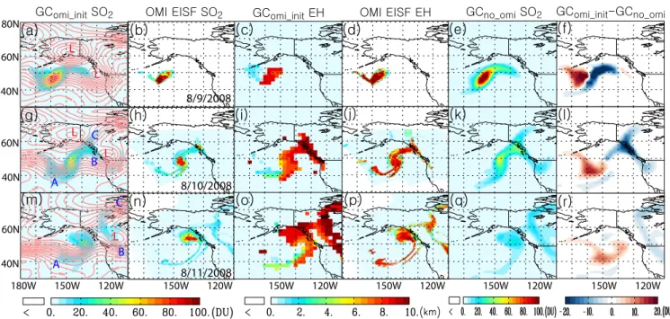
Fig. 2. (a)and(c): distribution of SO2column amount (in DU) and effective height (EH) (in km) of SO2on 9 August 2008 as simulated

by GEOS-Chem (GComi init) with model initiation of OMI EISF retrieved SO2on 8 August 2012;(b)and(d): the respective counterparts

of(a)and(c)retrieved from the OMI EISF algorithm;(e): same as(a)but from GEOS-Chem simulations without model initiation of EISF retrieved SO2(GCno omi), and(f)shows the difference between(a)and(e).(g)–(l)are respectively the same as(a)–(f)but for 10 August

2008.(m)–(r)are the same as(a)–(f)but for 11 August 2008. The pink solid lines in(a),(g)and(m)are isopleths (at 25 m intervals) of the 500 hPa geopotential height (in m). L in red in(a),(g)and(m)shows the location of low pressure systems, while A, B, and C in(g)and(m) respectively mark the three different transport pathways for SO₂. Subscripts omi init and no omi respectively denote the simulation with and without initialization of OMI SO2data.

ratio is in the range of 6–10 km. However, it also is noted that in model simulation by Kristiansen et al. (2010), the SO2emission is specified for two days at the model grid box

where Kasatochi is located, and hence their scheme for the initialization of emission is similar to this study, although no OMI SO2 retrieval are directly assimilated in their model.

Nevertheless, both the retrieval of SO2amount (such as those

from standard OMI product) and retrieval of SO2 height

(such as from research algorithm developed by Yang et al., 2009, 2010) have uncertainties with best estimate of 20 % and 1–2 km respectively; low bias in height retrieval often corresponds to high bias in SO2 amount retrieval, and vice

versa. To investigate the impact of the SO2injection height

(used after the OMI satellite overpass) on the simulation re-sults, sensitivity simulations are conducted with different in-jection heights of 2, 4, 6, and 8 km (Sect. 4.2).

3.2 Radiative forcing calculations and sensitivity analysis

Our forcing calculation follows Wang et al. (2008) but with improvement in the treatment of cloud effects. A four-stream broadband radiative transfer model (RTM), employ-ing monthly-mean surface reflectance data (Koelemeijer et al., 2003) and the simulated 3-D aerosol sulfate mass is

em-ployed for the forcing calculations (Fu and Liou, 1993; Wang et al., 2004). The RTM is applied to the solar spectrum for six bands, ranging from 0.2 to 4 µm. The GEOS-Chem simulated volcanic sulfate mass is converted to AOD following Wang et al. (2008) in which the hygroscopic effect on sulfate par-ticle size and refractive index is considered. Band averages of relative-humidity dependent single scattering properties of sulfate aerosols (e.g., single scattering albedo, extinction cross section, and asymmetry parameter) are tabulated in the RTM for computational expediency, while the cloud optical thickness is adopted from the GEOS-5 meteorological field. In the RTM calculations, all aerosol and cloud particles are assumed to be externally mixed (Wang et al., 2008). The dif-ference between upwelling solar irradiances calculated in the presence and absence of sulfate aerosols, without (with) con-sidering the cloud in the RTM calculation, is the clear-sky (all-sky) sulfate direct radiative forcing. In each grid cell, the forcing calculation is conducted every 6 hours because the input cloud properties have 6-hourly temporal resolution.

(7)

neutralized form of ammonium sulfate (Wang et al., 2008), stratospheric volcanic sulfate aerosols may less neutralized (more acid) and thus have greater hygroscopicity than tropo-spheric sulfate aerosols (Russell et al., 1996). Indeed, within 3–6 months after Pinatubo eruption, the effective radius (or equivalently, geometric mean radius assuming no change in geometric standard deviation) of stratospheric aerosols was shown an increase by a factor of 2–3 (Russell et al., 1996). Wang et al. (2008) estimated that for the same amount of sul-fate mass with the same size distribution at RH=5 %, am-monium sulfate, amam-monium bisulfate, and sulfate acid par-ticles can have 20-30 % difference among the radiative forc-ing efficiencies (normalized to sulfate mass) at RH = 80 %; this difference is primarily due to their different hygroscopic growth. To consider the uncertainty due to hygroscopicity and other factors (such as particle coagulation that are not included in the current GEOS-Chem simulation) in the esti-mate of particle size, we conducted sensitivity experiments to compute the forcing with different sets of sulfate opti-cal properties with increasing particle geometric radius from 0.07 µm to 0.19 µm (Sect. 3.3).

4 Results

4.1 Baseline results for SO2and volcanic sulfate AOD distribution

The model simulation shows that the SO2plume, as a whole,

moved toward the east after the eruption (Fig. 2a, g and m). The initial SO2 plume center at 52◦N, 165◦W on 8

Au-gust 2008 dispersed toward the southeast on 9 AuAu-gust 2008 (Fig. 2a) as a result of the southeastward rotation of the major-axis of the low pressure system (originally centered on 52◦N, 168◦W on Fig. 1c), and on 10 August moved 50◦N, 148◦W (Fig. 2e). From this center of SO2 mass on August

10, SO2plume extends in several directions (Fig. 2g): (i)

to-ward the southwest (e.g., location A in Fig. 2g) as a result of the blocking ridge along 130◦W, (ii) toward the northeast (location C) under the influence of a low-pressure system centered around 65◦N, 150◦W. However, the flow toward the northeast bifurcates at 55◦N, 135◦W, with one branch continuing northeast, while another branch moves southeast (location B in Fig. 2g) and then turns northwest in the west-erly anti-clockwise flow circulating around another low pres-sure system centered around 52◦_{N, 125}◦_{W. The general} SO2 distribution on 10 August (Fig. 2g) is maintained on

11 August, except that the SO2cloud is translated eastward

by∼10◦latitude with its center at 55◦N, 135◦W, and SO2

amounts are more diluted to 20–40 DU on average (Fig. 2m). Generally good agreement can be found between the mod-eled SO2spatial distribution (Fig. 2a, g and m) and the OMI

retrieved SO2amount (Fig. 2b, h and n), especially in terms

of the location of the volcanic cloud core on 9 August 2008 and the bifurcation of the SO2plume on both 11 and 12

Au-gust 2008. However, the modeled patterns overall are more diffuse than the OMI observations (Fig. 2), likely reflect-ing the difference between the GEOS-Chem model grid size (2◦×2.5◦) and the OMI footprint size (24 km×13 km at nadir) and the non-ideality in the model (as discussed below). In addition, the inability of OMI to retrieve SO2located

be-neath clouds also can partially explain why the flow of SO2

is not as continuous and smooth as that in the model simula-tions.

In addition to the overall agreement between modeled and OMI retrieved spatial distribution of SO2amount, the

GEOS-Chem modeled distribution of SO2effective height on 9–11

August 2008 (Fig. 2c, i, and o) is also consistent with the counterparts of OMI EISF retrievals (Fig. 2d, j, and p). Both model and OMI retrievals show that the core of SO2plume

was generally maintained at the effective height of 10 km, but the effective height for the part of SO2 plume in the

southwest direction (C in Fig. 2g and C in top-right corner of Fig. 2m) decent to about 2–4 km. In the comparison, it is noted that OMI is not sensitive to SO2plumes at low altitude.

Contrast between GEOS-Chem simulations with and with-out initialization of using OMI EISF SO2 data shows

sig-nificant differences (up to±20 DU) in the spatial pattern of SO2distribution (Fig. 2f, l, and r) during 9–11 August 2008.

However, in comparison to the OMI retrievals, it is clear that the simulation with the assimilation of OMI EISF SO2data

gives a better description of the SO2transport. The

simula-tion without assimilasimula-tion of OMI EISF SO2appears to give a

faster dilution of SO2from the core, and therefore, an

over-estimation of SO2in locations such as A, B, and C marked on

Fig. 2g and 2m (Fig. 2f, l, and r). In addition, in the southwest direction (along location A), the simulated SO2 without

as-similation reaches too far to the south (around 30◦_{N) on 10–} 11 August 2008, while both OMI and simulation with assimi-lation show the SO2plume only reaches around 38◦N.

Quan-titatively, the simulated SO2with assimilation have a

corre-lation coefficient of 0.73 and normalized root-mean square difference of (with respect to OMI retrievals) 1.25, while without assimilation respectively have 0.63 and 1.53, with OMI SO2(after re-gridding to GEOS-Chem grid). Such

im-provement through assimilation may be useful to short-term prediction of the movement of volcanic SO2, which can have

important implications for aviation weather forecast. Quantitative comparisons with OMI SO2 data show that

GEOS-Chem underestimates SO2 columns by over 20 DU

in the plume core on August 10, and by ∼60 DU on Au-gust 11 (Fig. 2). Further comparison of the 40-day time series of modeled and EISF-retrieved total SO2 burden

af-ter the eruption shows that the model underestimation ap-pears persistent throughout the simulation (Fig. 3). Figure 3a also shows that the modeled evolution of total SO2₄− mass is consistent with the temporal evolution of total SO2mass,

(8)

(a)

(b)

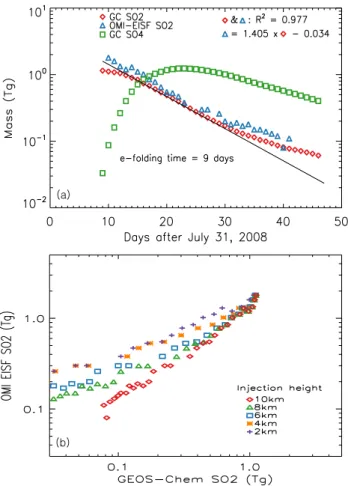
Fig. 3. (a)Time series of daily total volcanic SO2mass (in log-scale

on y-axis) after the Kasatochi eruption. Red diamonds and blue tri-angles are the results from the GEOS-Chem simulation and OMI retrievals, respectively. Also overlaid is the GEOS-Chem simulated total volcanic SO2₄−mass (green squares). The solid black line is a linear least-squares-fit between the GEOS-Chem simulated SO2

mass (log scale) and the number of days after the eruption, from which an e-folding time of 9 days for SO₂is derived. Also shown at the top right is the equation for a linear least-squares-fit between GEOS-Chem simulated and OMI retrieved SO2as well as their

lin-ear correlation coefficient (R).(b)Scattered diagram of daily to-tal volcanic SO2mass between GEOS-Chem (with each injection

height) and OMI retrievals. Note, the time series of OMI SO2data

is obtained from Krotkov et al. (2010), in which the data points in the first two days are estimated based upon the extrapolation to ac-count for OMI’s sampling bias due to limited spatial and temporal coverage.

7.5–12 km, and 40 % 12-14 km), their modeled averages of sulfate AOD over the Northern Hemisphere between 0◦_N and 85◦N for Kasatochi eruption peaked in early September centered around 7 September, which is about 9 days earlier than that is derived based upon OSIRIS AOD (at 750 nm) data. Figure 3 in Kravitz et al. (2012) further showed that the peak value (0.006) of zonal averages of OSIRIS AOD first appeared on 1September at 55◦N and then expanded to the northern latitude region in the following 30–40 days. It

is noted that the statistics from OSIRIS AOD data can be af-fected by its limitations in spatial and temporal sampling (be-cause OISIRIS is a limb sensor measuring the visible light). Furthermore, the value of averages of AOD not only depends on the SO2₄− mass, but also is subject to how SO2₄− mass is distributed spatially, the aerosol scattering properties and the relative humidity simulated or prescribed in the model. Hence, instead of using AOD or SO2₄−to quantitatively eval-uate the model, we conduct the quantitative comparison with SO2data derived from OMI, and further qualitatively

evalu-ate the model with AOD data from MODIS and CALIOP. Based on the OMI SO2data for 14–31 August 2008 (i.e.,

blue triangles in Fig. 3a), Krotkov et al. (2010) estimated an e-folding time for the Kasatochi SO2 of around 9 days.

Interestingly, an identical e-folding time is obtained in our GEOS-Chem model simulation for the same time period, which suggests that the oxidation rate for converting SO2

to sulfate (e.g., the first-order sink rate) in the upper tropo-sphere and low-level stratotropo-sphere has no systematic bias in the model, and is consistent with that derived from OMI re-trievals. However, the persistent underestimate in the mod-eled SO2 columns as shown in Figs. 2 and 3a may reflect

a larger sink term or overestimation of oxidant abundance during early plume evolution when SO2underwent

aqueous-phase oxidation in clouds. This hypothesis is evaluated be-low by comparing the cloud fraction and LWP in the GEOS-5 meteorological fields with those retrieved by MODIS be-cause in-cloud oxidation is a major sink for atmospheric SO2.

Figure 3b also illustrates the comparison of daily total SO2

mass between GEOS-Chem and OMI-EISF retrievals. As in-jection height is lowered from 10 through 2 km, the reduction rate of total SO2mass drastically increases with associated

e-folding time decreasing from 9 days to∼3 days, indicating that the life time of volcanic SO2more depends on injection

height rather than injected mass.

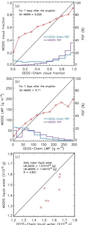
Figure 4a illustrates a cloud fraction comparison be-tween GEOS-Chem and MODIS for each cloud fraction bin (i.e., 0.1) over the region of SO2 cloud transport (30–70◦N

(9)

(c) (a)

(b)

Fig. 4.Comparison (red line) of Cloud fraction(a)and LWP (b) de-rived from GEOS-Chem and MODIS during 7 days after the erup-tion over the region (30–70◦N and 100–175◦W).(c)comparison of daily total amount of liquid water derived from GEOS-Chem and MODIS for the same time period and region. Also shown in(a) and(b)are the probability density function (PDF, right y-axis) for each cloud fraction (or LWP) bin from GEOS-Chem (blue line) and MODIS (purple line). In each panel, the linear correlation coeffi-cient (R) and the average difference between GEOS-Chem (GC) and MODIS are also provided.

(Fig. 4c), reflecting the relatively more important contribu-tion of (b), i.e., the overestimacontribu-tion of the number of thin and small clouds in GEOS-5. Presumably, it is those small and thin clouds that can more effectively interact with SO2

(because of their large area-to-volume ratio). Therefore, dur-ing the early period after the eruption, GEOS-Chem overesti-mates the abundance of liquid water clouds (or oxidants) able to convert volcanic SO2 into sulfate aerosols in the

simula-tion, which partially explains the model underestimation of SO2as shown in Fig. 3. This is especially likely after further

consideration that MODIS liquid water path may also has a positive bias (that is∼10 % in global averages over ocean when compared to the AMSR measurements) (Seethala and Horv´ath, 2010). Indeed, our sensitivity experiment shows that a reduction of liquid water path by 15 % in the first two days in GEOS-5 field results in a 5 % increase in SO2

to-tal amount (7 % and 3 % in 1st and 2nd day respectively). It is noted that once SO2reaches the upper troposphere and

stratosphere, its main sink is oxidation by OH, and hence the consistency of e-folding time between GEOS-Chem simula-tions and OMI observasimula-tions (Fig. 3) indicates that oxidation of SO2by OH is well represented in the model.

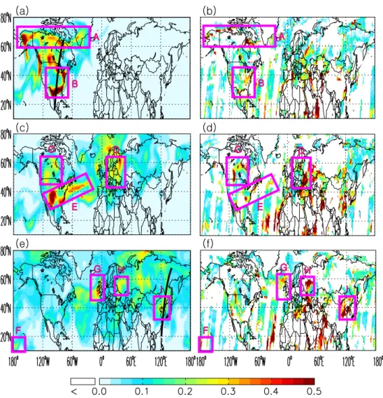
For further evaluation of the model, the simulated dis-tribution of volcanic sulfate AOD is compared with Terra and Aqua MODIS level-2 aerosol data on several selected days when the pathway of volcanic sulfate AOD is easily discernable (Fig. 5). On August 14 (8 days after the erup-tion), MODIS AOD maps indicate that the volcanic sul-fate aerosols (with mid-visible AOD>0.5) was mainly lo-cated over Alaska, Northern Canada, and Northern Mexico (marked respectively as regions A and B in Fig. 5b); such distributions are reasonably reproduced by the GEOS-Chem model simulation in Fig. 5a. The signature of volcanic sul-fate aerosols, two weeks after the volcanic eruption, can be further identified over the continental US, Western At-lantic Ocean, and Europe (respectively marked as C-E in both Fig. 5c and d). A period of about 10 days is enough to trans-port the volcanic aerosols not only over the entire Atlantic Ocean, but also over Asia. About 17 days after the eruption, the volcanic sulfate aerosols are transported zonally from Eu-rope to Eastern Asia (e.g., region G, H, and I in Fig. 5e) and even meridionally to the Southern Pacific Ocean (region F in Fig. 5e). Overall, Fig. 5 shows that the hemispheric distri-butions of the volcanic sulfate AOD from the simulation are comparable with the MODIS AOD observations.

In addition to using satellite data for evaluating model-simulated column amounts (such as total SO2 burden and

(10)

(a) (b)

(c) (d)

(e) (f)

A A

B B

C D C D

E E

F

G H

I

F

G _H

I

Fig. 5.Spatial distribution of volcanic sulfate aerosol optical depth (AOD) at 550 nm as simulated by GEOS-Chem (left column) and as retrieved by MODIS (right column) on 14 (top row), 19 (middle row), and 25 (bottom row) August 2008, respectively. The solid black lines in(a)and(e)respectively indicate the ground tracks of CALIOP data that are shown in Fig. 6a and c. The pink rectangles and letters highlight the regions of large volcanic AOD, as discussed in Sect. 4.1.

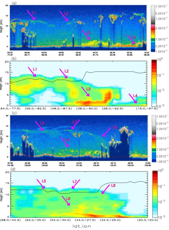
(black line in Fig. 6b) over North America. Within this layer, the CALIOP measurements of depolarization ratio at 530 nm and backscattering attenuation at 1062 nm both show nearly zero values, and CALIOP layer classification algorithm in-dicate that this layer are dominated by aerosols with small fraction of cirrus (figures now shown). The model simula-tion is able to capture a similar vertical distribusimula-tion of the volcanic sulfate aerosol extinction (marked as L1 and L2 in Fig. 6b), although the coarser model resolution in the strato-sphere cannot resolve the very thin-layer structure of the sul-fate aerosols detected by CALIOP data. The stratospheric sulfate aerosols are also distinctly detected by CALIPSO on the∼17th day after the eruption over East Asia (marked as L5, L6, and L8 in Fig. 6c), and those are plausibly captured by the GEOS-Chem simulation in Fig. 6d, especially the de-scending path of aerosols from Siberia, to East Asia, and to

the western North Pacific (marked respectively as L5, L6, and L8 in both Fig. 6c and d). In addition, CALIOP images in Fig. 6a and b also indicate the likely deposition of volcanic sulfate aerosols in the middle-to-lower atmosphere such as over the south central US (marked as L3 and L4 in Fig. 6a and b) and over northeast China (marked as G in Fig. 6c and d); these “touch down” features are also seen in the similar curtain plots showing the difference in GEOS-Chem simulation with and without considering volcanic aerosols, although non-volcanic aerosols from local source also con-tribute to the high loading of particles in regions L3 and L7 (figures now shown here).

(11)

(a)

(b)

(c)

(d)

1.0X10-1

1.0X10-2

1.0X10-3

1.0X10-4

5.0X10-2

5.0X10-3

5.0X10-4

1.0X10-1

1.0X10-2

1.0X10-3

1.0X10-4

5.0X10-2

5.0X10-3

5.0X10-4

L1 _L2

L3

L4

L1

L2

L3

L4

L5 L7

L6

L8

L5 L7

L6

L8

10-3 10-2 10-1 100

Fig. 6. (a)vertical distribution of 532 nm total attenuated backscatter (km−1sr−1) measured by the CALIOP lidar, and(b)the corresponding distribution of tropopause (black line) and the simulated sulfate aerosol extinction coefficient (km−1) at 550 nm for the CALIPSO ground track in Fig. 5a on 14 August 2008.(c)and(d)are respectively the same as(a)and(b)for the CALIPSO ground track solid black line in Fig. 5e. The pink arrows and letters highlight the regions of large volcanic AOD, as discussed in Sect. 4.1.

sulfate aerosol in the entire atmosphere (Fig. 7a) with a sig-nificant fraction of the aerosol in the stratosphere (Fig. 7b). The GEOS-Chem simulated sulfate AOD is compared with AOD from CALIPSO in Fig. 7c and d only for altitudes over 10 km to minimize the influence of non-volcanic sul-fate aerosols in the CALIOP data. It is apparent that the model produces a comparable AOD (mean AOD is∼0.06)

(12)

(a)

(d) (c) (b)

Fig. 7. (a)Temporal evolution of zonally averaged volcanic sulfate aerosol optical depth (SAOD) from GEOS-Chem simulations,(b) same as(a)but for SAOD above 10 km from the surface,(c)the same as(b)but SAOD sampled along the CALIOP ground track, and(d)same as(c)but based upon the analysis of CALIOP level-2 aerosol layer product with the consideration of data quality flags.

algorithm; indeed, the temporal evolution of the zonally aver-aged backscattering ratio from CALIOP as shown in Vernier et al. (2011) is more similar to the GEOS-Chem simulation in Fig. 7b. In addition, as discussed in Heard et al. (2012), volcanic sources other than Kasatochi, such as the ongoing eruption from Kilauea volcano (19.4◦N, 155.3◦W) in 2008

may also contribute to the slower decrease of AOD above 10 km in the CALIOP data. About 70 days after the erup-tion, stratospheric aerosol is no longer detected in satellite data over middle and high latitudes, and the simulated sulfate AOD is also very small (∼4×10−4). About 100 days after the eruption, the stratospheric sulfate AOD in the model is negligible with daily values of 10−4.

4.2 Baseline results for volcanic sulfate forcing

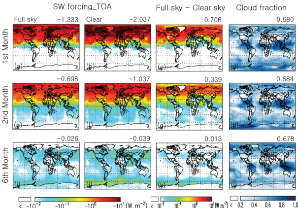
Figure 8 shows the monthly averaged direct shortwave (SW) radiative forcing by the volcanic sulfate aerosols at the top of the atmosphere (TOA) after the Kasatochi eruption. In monthly and global averages, the clear sky and all sky short-wave forcing of volcanic sulfate aerosols are both strongest (i.e., most negative) in the first month after the eruption, with respective values of−2.0 W m−2_and

−1.3 W m−2_{(Fig. 8a–}

b); they steadily become weaker with respective values of

−1.0 and−0.7 W m−2in the second month (Fig. 8e–f), and

−0.04 and−0.03 in the 6th month (Fig. 8i–j). Geograph-ically, the volcanic sulfate aerosols are not transported to the Southern Hemisphere until the 2nd month after the erup-tion, and do not spread over the whole Southern Hemisphere until 30 September 2008. Indeed, most of the volcanic sul-fate aerosols remained north of 20◦N in the first month af-ter the eruption (Fig. 8a). The difference in radiative forc-ing between clear and all sky depends, to a large extent, on the cloud fraction and relative altitude of the sulfate aerosol layer and clouds. Since sulfate particles and cloud droplets are highly scattering at visible wavelengths where the solar spectrum peaks, cloud layers, whether underlying or overly-ing the aerosol layer, generally reduce the spectral contrast between the bright aerosol layer and darker land/ocean sur-face when viewed from the TOA. As such, cloud layers often reduce the clear-sky radiative forcing of scattering aerosols (Wang et al., 2008). Hence, comparing the third and fourth columns in Fig. 8c, g and k show that the difference between clear-sky and all-sky radiative forcing is small (large) in re-gions where cloud fraction is low (high) such as over the Sa-haran desert and the dry regions of the central-to-east Pa-cific (cloudy regions include the southern ocean at 40–60◦S, the tropics, and high latitudes). As expected, over Greenland where surface albedo is high (radiatively acting like a cloud layer), the clear and cloudy sky forcing is nearly the same.

A daily time series of global averages of sulfate aerosol all-sky radiative forcing at the TOA is shown in Fig. 9. Soon after the Kasatochi eruption, the continuous conversion of SO2into sulfate results in a steady increase of sulfate AOD

(13)

z~G{vh

mG TXUZZZ j

TWU]`_

TWUWY]

TYUWZ^

TXUWZ^

TWUWZ`

XGt

YGt

]Gt

T T T T

jG GWU]_W

GWU]_[

GWU]^_ GWU^W]

GWUZZ`

GWUWXZ mG GTGjG

OP OP OP OP

Fig. 8.Averages of volcanic sulfate shortwave (SW) radiative forcing (Wm−2) at the top of the atmosphere (TOA) for all sky(a)and clear sky(b)conditions, as well as their differences(c)in the first month (a–c), second month(e–g), and the 6th month(i–k)after the Kasatochi eruption on 8 August 2008. Also shown are the corresponding distributions of cloud fraction (d,handl). Denoted on the top right of each panel is the global average (weighted by gridbox area) of the corresponding quantity.

Fig. 9.Temporal evolutions of the daily, global mean volcanic sul-fate radiative forcing (Wm−2) at the top of the atmosphere (TOA) for 5 different volcanic SO2injection heights ranging from 10 km

(shown in red line) to 2 km (shown in purple) with interval of 2 km (see legend on the top right for details). Also shown in the legend, corresponding to each injection height used in the GEOS-Chem simulation, are days (after the eruption on 8 August 2008) when the peak of the shortwave forcing occurs.

1991 (Minnis et al., 1993). The significant larger effect of Pinatubo eruption on climate is in part due to the following factors: (a) it ejected∼30 Tg of SO2up to 30 km above the

sea level, most of which concentrated in 20–27 km altitude (McCormick et al., 1995); (b) at this altitude range over the subtropics, the intensity of planetary wave activity and the phase of the quasi-biennial oscillation regulates the poleward transport, but were shown to be not effective in the North-ern Hemisphere in June–July 1992; (c) the spread of SO2to

the subtropics in Southern Hemisphere is found to be unex-pectedly faster in June–July 1991, which is attributed to the abnormality of the planetary wave activates over the equa-tor and southern subtropics (Trepte et al., 1993); (d) conse-quently, SO2amount was mainly located in the 30◦N–30◦S

(14)

(McCormick et al., 1995). Consequently, Kasatochi eruption may have only affected the global radiative energy budget for about 100 days, and has much less impact on climate.

The timeline of our simulated volcanic sulfate forcing is consistent with model experiment’s by Kravitz et al. (2012) that showed all volcanic sulfate aerosols might have been de-posited out of the atmosphere by February 2009, and the no-ticeable forcing may deceased even quicker. A direct quanti-tative comparison with the results from Kravitz et al. (2012) is complicated by: (a) the model difference in spatial resolu-tion and temporal resoluresolu-tion (4◦×5◦and focus of monthly scale in their climate model), chemical mechanisms (only prescribed OH field available in their model to oxidize SO2

in the stratosphere), and cloud fields (simulated solely with a climate model), and (b) the definition of sulfate forcing in which aerosol forcing feedback on stratospheric thermal adjustment are considered in their model. Nevertheless, be-cause of sulfate particle is highly scattering (with the single scattering albedo value close to 1) in visible and other short-wave spectrum, our estimate of global forcing at the TOA and surface is very similar, with a global averages of−1.3 Wm−2 in August and−0.7 Wm−2forcing in September, which ap-pear consistent with results in Kravitz et al. (2012) showing a−2 Wm−2of zonal averages of forcing at the surface over the Northern Hemisphere in August and September.

4.3 Sensitivity experiment to SO2injection height

In order to investigate the effect of volcanic SO2plume

in-jection height on SW radiative forcing, we conducted sensi-tivity simulations with injection heights of 2, 4, 6 and 8 km. Figure 9 shows that the radiative forcing has a strong depen-dence on the volcanic SO2injection height. As the injection

height decreases, the magnitude and the duration of the forc-ing decreases. For example, for a 2 km injection height, the peak forcing is−0.6 W m−2 and the sulfate aerosols influ-ence SW radiation for about 35 days, which contrasts with

−2.1 W m−2and about 100 days when injection height is set at 10 km.

Since the temporal evolution of the volcanic sulfate SW radiative forcing shown in Fig. 9 appears to follow a lognor-mal distribution, the following function is found to provide a good fit to the forcing-time curves in Fig. 9 for different injection heights:

y=S1e

−2(ln xS2)2

xS2 q

π

2 ,

where x=injection height (km), y=parameterized ra-diative forcing (W m−2), and the two scale factors are a function of injection height x: S1= 0.4x + 0.5, and

S2=−0.00375x + 0.0875. It is found that the parameterized

SW radiative forcing agrees with the GEOS-Chem simu-lated forcing for each injection height as a function of num-ber of days after the eruption, with linear correlation

coeffi-cients generally larger than 0.98 (Fig. not shown). As shown in Fig. 10, the parameterization adequately reproduces the peak value of the radiative forcing (Fig. 10b) and the timing for this peak value (Fig. 10a) for different injection heights. Based upon this parameterization, a difference of 2 km in in-jection height can lead to a 0.4 % difference in the overall es-timate of the forcing effect (e.g., forcing multiplied by time) in the whole globe.

4.4 Sensitivity experiment to aerosol size distribution

In our baseline simulation, the sulfate particles are assumed to have a lognormal size distribution with a geometric radius of 0.07 µm and standard deviation of 1.8 µm. In order to in-vestigate the impact of volcanic sulfate particle size on SW radiative forcing at the TOA, sensitivity experiments were conducted to compute the forcing with different sets of sul-fate optical properties corresponding to increasing geometric radii from 0.07 µm to 0.19 µm with a step size of 0.03 µm. Wang et al. (2008) showed that as the particle size increases, the associated increase in particle extinction cross section outweighs the associated reduction in backscattering, and thus results in stronger aerosol forcing. As shown in Fig. 11, an increment of 0.03 µm in sulfate particle radius results in an enhancement of∼0.1-0.2 W m−2in the 30-day (after erup-tion) and global average sulfate all-sky SW radiative forcing at the TOA.

5 Summary and discussion

GEOS-Chem, a global chemical transport model, has been used in conjunction with constraints from the OMI-EISF re-trievals of SO2amount and effective height to simulate the

life cycle of SO2and volcanic sulfate aerosols after the 2008

Kasatochi eruption and to study the resultant impact on di-rect shortwave radiative forcing. With the use of the OMI EISF-based SO2product to initialize the SO2distribution in

GEOS-Chem, the simulated lifetime (with an estimated e-folding time of 9 days) as well as the spatial distribution and temporal evolution of the volcanic SO2burden in the

atmo-sphere after the eruption are both in good agreement with OMI SO2observations, suggesting that the oxidation of SO2

in the stratosphere (primarily by the hydroxyl radical, OH) is reliably represented in GEOS-Chem. However, a consis-tent low (∼25 %) bias is found in the GEOS-Chem simulated SO2burden, and comparison with MODIS cloud products

in-dicates that this is likely due to a high (∼20 %) bias in cloud liquid water amount and a resultant stronger oxidation of SO2

in the GEOS meteorological data during the first week after the eruption when part of SO2is oxidized by clouds. Further

(15)

(a) (b)

Fig. 10. (a)Scatter plot of the volcanic SO₂ injection height (km) and the days (after the eruption) when the peak of daily and global averages of volcanic sulfate shortwave forcing occurs. The data are based upon results in Fig. 9.(b)same as(a)but shows the peak value of the daily and global average of volcanic sulfate shortwave forcing. The red lines in(a)and(b)respectively show the results based upon the parameterizations as described in Sect. 4.3.

Fig. 11.Global and 30-day (after eruption) average of volcanic sul-fate shortwave forcing at the top of atmosphere as a function of the geometric radius (rg) used in the log-normal size distribution to

de-scribe the aerosol optical properties in the forcing calculation.

then to the south central Great Plains in the first two weeks, as well as (b) their zonal transport from high-latitude regions of North America to mid- and high-latitude regions in Eu-rope and Asia, and the consequent transport from Siberia to southeast China within three weeks after the eruption.

Radiative transfer calculations show that the all-sky direct radiative forcing at the TOA due to the Kasatochi volcanic sulfate aerosols reached a peak in the late second week and early third week post-eruption, with a daily, global average value of∼2 W m−2. Consequently, in global and monthly av-erages, the volcanic sulfate forcing from the Kasatochi erup-tion peaks up to −1.3 W m−2 in the first month after the eruption, with majority of the forcing-influenced region

lo-cated north of 20◦_{N; and then gradually weakens to less} than−0.1 W m−2 _{four months after the eruption. The}

vol-canic aerosol forcing doesn’t influence the entire Northern Hemisphere until the middle of the second month after the eruption. It is found that clouds can effectively reduce the magnitude of the volcanic sulfate forcing by 20–40 %, on av-erage.

Sensitivity analysis shows that accurate description of the SO2injection height and the initial 3-D distribution of SO2

in the CTM are both critical for reliable simulation of the lifetime and spatiotemporal distribution of volcanic SO2and

aerosols after the eruption. For the Kasatochi eruption, it is shown that the temporal evolution of the volcanic sulfate forcing can be parameterized using a log-normal distribution as a function of injection height and number of days after the eruption. This parameterization indicates that every 2 km re-duction of SO2injection height results in a 2 day decrease in

SO2lifetime and 0.4 W m−2reduction in forcing (in global

and daily averages). Further sensitivity tests also showed that every 0.03 µm increase of geometric particle radius used in the log-normal size distribution for describing aerosol opti-cal properties leads to∼25 % increase in the magnitude of the forcing, although the rate of increase falls off for larger geometric radii.

This study is among the first to assimilate both satellite-based SO2plume height and column amount into a CTM for

an improved simulation of volcanic SO2transport, which has

(16)

Acknowledgements. This study is supported by NASA At-mospheric Chemistry Modeling and Analysis Program (NNX10AG60G) managed by Richard S. Eckman, and NASA Radiation Sciences Program managed by Hal B. Maring.

Edited by: M. Kopacz

References

Ackerman, S. A., Strabala, K. I., Menzel, W. P., Frey, R. A., Moeller, C. C., and Gumley, L. E.: Discriminating clear sky from clouds with MODIS, J. Geophys. Res., 103, 32141–32157, 1998. Alexander, B., Park, R. J., Jacob, D. J., and Gong, S.: Transition

metal-catalyzed oxidation of atmospheric sulfur: global impli-cations for the sulfur budget, J. Geophys. Res., 114, D02309, doi:10.1029/2008JD010486, 2009.

Andres, R. J. and Kasgnoc, A. D.: A time-averaged inventory of subaerial volcanic sulfur emissions, J. Geophys. Res., 103, 25251–25261, 1998.

Barnes, S. L.: A technique for maximizing details in numerical weather map analysis, J. Appl. Meteor., 3, 396–409, 1964. Bey, I., Jacob, D. J., Yantosca, R. M., Logan, J. A., Field, B., Fiore,

A. M., Li, Q., Liu, H., Mickley, L. J., and Schultz, M.: Global modeling of tropospheric chemistry with assimilated meteorol-ogy: Model description and evalustion, J. Geophys. Res., 106, 23073–23096, 2001.

Bond, T. C., Bhardwaj, E., Dong, R., Jogani, R., Jung, S., Ro-den, C., Streets, D. G., and Trautmann, N. M.: Historical emis-sions of black and organic carbon aerosol from energy-related combustion, 1850–2000, Global Biogeochem. Cy., 21, GB2018, doi:10.1029/2006GB002840, 2007.

Budyko, M. I.: Climatic Changes, AGU, Washington, DC, USA, 261 pp., doi:10.1029/SP010, 1977.

Burrows, J. P., Weber, M., Buchwitz, M., Rozanov, V., Ladst¨atter-Weißenmayer, A., Richter, A., DeBeek, R., Hoogen, R., Bram-stedt, K., Eichmann, K.-U., Eisinger, M. and Perner, D.: The Global Ozone Monitoring Experiment (GOME): Mission con-cept and first scientific results, J. Atmos. Sci., 56, 151–175, 1999. Carn, S. A., Krueger, A. J., Bluth, G. J. S., Schaefer, S. J., Krotkov, N. A., Watson, I. M., and Datta, S.: Volcanic eruption detection by the Total Ozone Mapping Spectrometer (TOMS) instruments: A 22-year record of sulphur dioxide and ash emissions, in Vol-canic Degassing, edited by: Oppenheimer, C., Pyle, D. M., and Barclay, J., Spec. Publ. Geol. Soc. Ldn, 213, 177–202, 2003. Chin, M., Jacob, D. J., Gardner, G. M., Foreman-Fowler, M. S., and

Spiro, P. A.: A global three-dimensional model of tropospheric sulfate, J. Geophys. Res., 101, 18667–18690, 1996.

Clarisse, L., Coheur, P. F., Prata, A. J., Hurtmans, D., Razavi, A., Phulpin, T., Hadji-Lazaro, J., and Clerbaux, C.: Tracking and quantifying volcanic SO2 with IASI, the September 2007 eruption at Jebel at Tair, Atmos. Chem. Phys., 8, 7723–7734, doi:10.5194/acp-8-7723-2008, 2008.

Deshler, T., Anderson-Sprecher, R., Jager, H., Barnes, J., Hofmann, D. J., Clemesha, B., Simonich, D., Osborn, M., Grainger R. G.,, and Godin-Beekmann, S.: Trends in the non-volcanic component of stratospheric aerosol over the period 1971–2004, J. Geophys. Res., 111, D01201, doi:10.1029/2005JD006089, 2006.

Eckhardt, S., Prata, A. J., Seibert, P., Stebel, K., and Stohl, A.: Esti-mation of the vertical profile of sulfur dioxide injection into the

atmosphere by a volcanic eruption using satellite column mea-surements and inverse transport modeling, Atmos. Chem. Phys., 8, 3881–3897, doi:10.5194/acp-8-3881-2008, 2008.

Evans, M. J. and Jacob, D. J.: Impact of new laboratory studies of N2O5 hydrolysis on global model budgets of tropospheric nitro-gen oxides, ozone, and OH, Geophys. Res. Lett., 32, L09813, doi:10.1029/2005GL022469, 2005.

Fisher, J. A., Jacob, D. J., Wang, Q., Bahreini, R., Carouge, C. C., Cubison, M. J., Dibb, J. E., Diehl, T., Jimenez, J. L., Leibensperger, E. M., Lu, Z., Meinders, M. B. J., Pye, H. O. T., Quinn, P. K., Sharma, S., Streets, D. G., van Donkelaar, A., and Yantosca, R. M.: Sources, distribution, and acidity of sulfate-ammonium aerosol in the Arctic in winter-spring, Atmos. Envi-ron., 45, 7301–7318, 2011.

Fairlie, T. D., Jacob, D. J., Dibb, J. E., Alexander, B., Avery, M. A., van Donkelaar, A., and Zhang, L.: Impact of mineral dust on nitrate, sulfate, and ozone in transpacific Asian pollution plumes, Atmos. Chem. Phys., 10, 3999–4012, doi:10.5194/acp-10-3999-2010, 2010.

Fu, T.-M., Jacob, D. J., Wittrock, F., Burrows, J. P., and Vrekoussis, M.: Global budgets of atmospheric glyoxal and methylglyoxal, and implications for formation of secondary organic aerosols, J. Geophys. Res., 113, D15303, doi:10.1029/2007JD009505, 2008. Frey, R. A., Ackerman, S. A., Liu, Y., Strabala, K. I., Zhang, H., Key, J. R., and Wang, X.: Cloud detection with MODIS, part I: Improvements in the MODIS cloud mask for collection, 5, J. Atmos. Ocean. Technol., 25, 1057–1072, 2008.

Fu, Q. and Liou, K. N.: Parameterization of the radiative properties of cirrus clouds, J. Atmos. Sci., 50, 2008–2025, doi:10.1175/1520-0469(1993)050<2008:POTRPO>.0.CO;2, 1993.

Hansen, J. E., Wang, W.-C., and Lacis, A. A.: Mount Agung pro-vides a test of a global climatic perturbation, Science,199, 1065– 1068, 1978.

Heard, I. P. C., Manning, A. J., Haywood, J. M., Witham, C., Red-ington, A., Jones, A., Clarisse, L., and Bourassa, A.: A com-parison of atmospheric dispersion model predictions with ob-servations of SO2and sulphate aerosol from volcanic eruptions,

J. Geophys. Res., 117, D00U22, doi:10.1029/2011JD016791, 2012.

Hofmann, D. J. and Solomon, S.: Ozone destruction through het-erogeneous chemistry following the eruption of El Chichon, J. Geophys. Res., 94, 5029–5041, doi:10.1029/JD094iD04p05029, 1989.

Intergovernmental Panel on Climate Change (2007), Climate Change 2007: The Physical Science Basis. Contribution of Working Group I to the Fourth Assessment. Report of the Inter-governmental Panel on Climate Change, edited by S. Solomon et al., Cambridge Univ. Press, Cambridge, UK

Karagulian, F., Clarisse, L., Clerbaux, C., Prata, A. J., Hurtmans, D., and Coheur, P. F.: Detection of volcanic SO₂, ash, and H₂SO₄ using the Infrared Atmospheric Sounding Interferometer (IASI), J. Geophys. Res., 115, D00L02, doi:10.1029/2009JD012786, 2010.

(17)

Koelemeijer, R. B. A., de Haan, J. F., and Stammes, P.: A database of spectral surface reflectivity in the range 335–772 nm derived from 5.5 years of GOME observations, J. Geophys. Res., 108, 4070, doi:10.1029/2002JD002429, 2003.

Kravitz, B., Robock, A., Bourassa, A., and Stenchikov, G.: Negligible climatic effects from the 2008 Okmok and Kasatochi volcanic eruptions, J. Geophys. Res., 115, D00L05, doi:10.1029/2009JD013525, 2010.

Krotkov, N. A., Schoeberl, M. R., Morris, G. A., Carn, S., and Yang, K.: Dispersion and lifetime of the SO₂cloud from the Au-gust 2008 Kasatochi eruption, J. Geophys. Res., 115, D00L20, doi:10.1029/2010JD013984, 2010.

Krueger, A. J.: Sighting of El Chichon sulfur dioxide clouds with the Nimbus 7 Total Ozone Mapping Spectrometer, Science, 220, 1277–1379, 1983.

Krueger, A. J., Walter, L. S., Bhartia, P. K., Schnetzler, C. C., Krotkov, N. A., Sprod, I., and Bluth, G. J. S.: Volcanic sulfur dioxide measurements from the Total Ozone Mapping Spectrom-eter (TOMS) instruments, J. Geophys. Res., 100, 14057-14076, 1995.

Kruger, A. J., Schaefer, S., Krotkov, N., Bluth, G., and Barker, S.: Ultraviolet remote sensing of volcanic emissions and applica-tions to aviation hazard mitigation Remote Sensing of Active Volcanism, Geophys. Monogr., 116, 25–43, 2000.

Lee C., Martin, R. V., van Donkelaar, A., Lee, H., Dickerson, R. R., Hains, J. C., Krotkov, N., Richter, A., Vinnikov, K., and Schwab, J. J.: SO2 emissions and lifetimes: Estimates

from inverse modeling using in situ and global, space-based (SCIAMACHY and OMI) observations, J. Geophys. Res., 116, D06304, doi:10.1029/2010JD014758, 2011.

Levelt, P. F., Hilsenrath, E., Leppelmeier, G. W., van den Oord, G. H. J., Bhartia, P. K., Tamminen, J., de Haan, J. F., and Veefkind, J. P.: Science objectives of the Ozone Monitoring In-strument, IEEE Trans. Geosci. Remote Sens., 44, 1199–1208, doi:10.1109/TGRS.2006.872336, 2006.

Liu, H., Jacob, D. J., Bey, I., and Yantosca, R. M.: Constraints from

210_{Pb and}7_{Be on wet deposition and transporting a global}

three-dimensional chemical tracer model driven by assimilated meteo-rological fields, J. Geophys. Res., 106, 12109–12128, 2001. Mari, C., Jacob, D. J., and Bechtold, P.: Transport and scavenging

of soluble gases in a deep convective cloud, J. Geophys, Res., 105, 22255–22267, 2000.

McLinden, C. A., Olsen, S. C., Hannegan, B., Wild, O., Prather, M. J., and Sundet, J.: Stratospheric ozone in 3-D models: a simple chemistry and the cross-tropopause flux, J. Geophys. Res., 105, 14653–14665, 2000.

Min, Q., Joseph, E., Lin, Y., Min, L., Yin, B., Daum, P. H., Klein-man, L. I., Wang, J., and Lee, Y.-N.: Comparison of MODIS cloud microphysical properties with in-situ measurements over the Southeast Pacific, Atmos. Chem. Phys., 12, 11261–11273, doi:10.5194/acp-12-11261-2012, 2012.

Minnis, P., Harrison, E. F., Stowe, L. L., Gibson, G. G., Denn, F. M., Doelling, D. R., and Smith Jr., W. L.: Radiative climate forcing by the Mount Pinatubo eruption, Science, 259, 1411–1415, 1993. Munro, R., Eisinger, M., Anderson, C., Callies, J., Corpaccioli, E., Lang, R., Lefebvre, A., Livschitz, Y., P´erez Albi˜nana, A.: GOME-2 on MetOp,Proc. The 2006 EUMETSAT Meteorologi-cal Satellite Conference, Helsinki, Finland, EUMETSAT, 48 pp., 92-9110-076-5, 2006.

Olivier, J. G. J. and Berdowski, J. J. M.: Global emissions sources and sinks, In: Berdowski, J., Guicherit, R. and B. J. Heij (eds.), The Climate System, 33–78 pp., Lisse, The Netherlands, 2001. McCormick, M., Thomason, L. W., and Trepte, C. R.: Atmospheric

effects of the Mt Pinatubo eruption, Nature, 373, 399–404, 1995. Pieri, D. and Abrams, M.: ASTER watches the world’s volcanoes: a new paradigm for volcanological observations from orbit, J. Volcanol. Geotherm. Res., 135, 13–28, 2010.

Prata, A. J. and Bernardo, C.: Retrieval of volcanic SO2 column

abundance from Atmospheric Infrared Sounder data, J. Geophys. Res., 112, D20204, doi:10.1029/2006JD007955, 2007.

Price, C. and Rind, D.: A simple lightning parameterization for calculating global lightning distributions, J. Geophys. Res., 97, 9919–9933, 1992.

Remer, L. A., Kaufman, Y. J., Tanr´e, D., Mattoo, S., Chu, D. A., Martins, J. V., Li, R.-R., Ichoku, C., Levy, R. C., Kleidman, R. G., Eck, T. F., Vermote, E., and Holben, B. N.: The MODIS Aerosol Algorithm, Products, and Validation, J. Atmos. Sci., 62, 947–973, 2005.

Rix, M., Valks, P., Hao, N., Loyola, D., Schlager, H., Huntrieser, H., Flemming, J., Koehler, U., Schumann, U., and Inness, A.: Volcanic SO2, BrO and plume height estimations using

GOME-2 satellite measurements during the eruption of Ey-jafjallaj¨okull in May 2010, J. Geophys. Res., 117, D00U19, doi:10.1029/2011JD016718, 2012.

Robock, A.: Volcanic Eruptions and Climate, Rev. Geophys., 38, 191–219, doi:10.1029/1998RG000054, 2000.

Russell, J. M., Luo, M. Z., Cicerone, R. J., and Deaver, L. E.: Satel-lite Confirmation of the Dominance of Chloroflourocarbons in the Global Stratospheric Chlorine Budget, Nature, 379, 526–529, 1996.

Russell, P. B. et al.: Global to microscale evolution of the Pinatubo volcanic aerosol derived from diverse measurements and analy-ses, J. Geophys. Res., 101, 18745-18763, 1996.

Seethala, C. and Horv´ath, ´A.: Global assessment of AMSR-E and MODIS cloud liquid water path retrievals in warm oceanic clouds, J. Geophys. Res., 115, D13202, doi:10.1029/2009JD012662, 2010.

Seinfeld, J. H. and Pandis, S. N.: Atmospheric Chemistry and Physics: From Air Pollution to Climate Change, 1203pp., John Wiley, Hoboken, NJ, USA, 2006.

Simkin, T. and Siebert, L.: Volcanoes of the World, 2nd edition. Geoscience Press in association with the Smithsonian Institution Global Volcanism Program, 368 pp., Tucson, AZ, USA, 1994. Solomon, S.: Stratospheric Ozone Depletion: a Review of Concepts

and History, Rev. Geophys., 37, 275–316, 1999.

Solomon, S., Daniel, J. S., Neely III, R. R., Vernier, J.-P., Dut-ton, E. G., and Thomason, L. W.: The Persistently Variable “Background” Stratospheric Aerosol Layer and Global Climate Change, Science, 333, 866–870, 2011.

Spiro, P. A., Jacob, D. J., and Logan, J. A.: Global Inventory of Sulfur Emissions with a 1◦×1◦ Resolution, J. Geophys. Res., 97, 6023–6036, 1992.

Toon, O. B.: Volcanoes and climate, Atmospheric Effects and Po-tential Climatic Impact of the 1980 Eruptions of Mount St. He-lens, edited by A. Deepak, NASA Conf. Publ., 2240, 15–36, 1982.

(18)

98, 18563–18573, 1993.

van der Werf, G. R., Morton, D. C., DeFries, R. S., Giglio, L., Ran-derson, J. T., Collatz, G. J., and Kasibhatla, P. S.: Estimates of fire emissions from an active deforestation region in the southern Amazon based on satellite data and biogeochemical modelling, Biogeosciences, 6, 235–249, doi:10.5194/bg-6-235-2009, 2009. Vernier, J.-P., Thomason, L. W., Pommereau, J.-P., Bourassa, A., Pelon, J., Garnier, A., Hauchecorne, A., Blanot, L., Trepte, C., Degenstein, D., and Vargas, F.: Major influence of trop-ical volcanic eruptions on the stratospheric aerosol layer during the last decade, Geophys. Res. Lett., 38, L12807, doi:10.1029/2011GL047563, 2011.

Wang, J., Jacob, D. J., and Martin, S. T.: Sensitivity of sulfate direct climate forcing to the hysteresis of particle phase transitions, J. Geophys. Res., 113, D11207, doi:10.1029/2007JD009368, 2008. Wang, J., Nair, U., and Christopher, S. A.: GOES-8 aerosol opti-cal thickness assimilation in a mesosopti-cale model: Online integra-tion of aerosol radiative effects, J. Geophys. Res., 109, D23203, doi:10.1029/2004JD004827, 2004.

Watson, I. M., Realmuto, V. J. Rose,, W. I., Prata, A. J., Bluth, G. J. S., Gu, Y., Bader, C. E., and Yu, T.: Thermal infrared re-mote sensing of volcanic emissions using the moderate reso-lution imaging spectroradiometer, J. Volcanol. Geotherm. Res., 135, 75–89, 2004.

Wesely, M. L.: Parameterization of surface resistance to gaseous dry deposition in regional-scale numerical models, Atmos. Environ., 23, 1293–1304, 1989.

Wilcox, E. M., Harshvardhan, and Platnick, S.: Estimate of the im-pact of absorbing aerosol over cloud on the MODIS retrievals of cloud optical thickness and effective radius using two inde-pendent retrievals of liquid water path, J. Geophys. Res., 114, D05210, doi:10.1029/2008JD010589, 2009.

Wu, S., Mickley, L. J., Jacob, D. J., Logan, J. A., and Yantosca, R. M.: Why are there large differences between models in global budgets of tropospheric ozone?, J. Geophys. Res., 112, D05302, doi:10.1029/2006JD007801, 2007.

Yang, K., Krotkov, N. A., Krueger, A. J., Carn, S. A., Bhar-tia, P. K., and Levelt, P. F.: Retrieval of large volcanic SO2 columns from the Aura Ozone Monitoring Instrument:

comparison and limitations, J. Geophys. Res., 112, D24S43, doi:10.1029/2007JD008825, 2007.

Yang, K., Krotkov, N. A., Krueger, A. J., Carn, S. A., Bhartia, P. K., and Levelt, P. F.: Improving retrieval of volcanic sulfur diox-ide from backscattered UV satellite observations, Geophys. Res. Lett., 36, L03102, doi:10.1029/2008GL036036, 2009.

Yang, K., Liu, X., Bhartia, P. K., Krotkov, N., Carn, S., Hughes, E., Krueger, A., Spurr, R., and Trahan, S.: Direct retrieval of sulfur dioxide amount and altitude from spacebornehyperspectral UV measurements: Theory and application, J. Geophys. Res., 115, D00L09, doi:10.1029/2010JD013982, 2010.