SRef-ID: 1684-9981/nhess/2005-5-799 European Geosciences Union
© 2005 Author(s). This work is licensed under a Creative Commons License.
and Earth
System Sciences
Modelling debris flows down general channels
S. P. Pudasaini, Y. Wang, and K. Hutter
Department of Mechanics – AG III, Darmstadt University of Technology, Hochschulstrasse 1, 64289, Germany Received: 2 June 2005 – Revised: 8 August 2005 – Accepted: 9 September 2005 – Published: 26 October 2005
Abstract. This paper is an extension of the single-phase cohesionless dry granular avalanche model over curved and twisted channels proposed by Pudasaini and Hutter (2003). It is a generalisation of the Savage and Hutter (1989, 1991) equations based on simple channel topography to a two-phase fluid-solid mixture of debris material. Important terms emerging from the correct treatment of the kinematic and dynamic boundary condition, and the variable basal topog-raphy are systematically taken into account. For vanish-ing fluid contribution and torsion-free channel topography our new model equations exactly degenerate to the previ-ous Savage-Hutter model equations while such a degenera-tion was not possible by the Iverson and Denlinger (2001) model, which, in fact, also aimed to extend the Savage and Hutter model. The model equations of this paper have been rigorously derived; they include the effects of the curva-ture and torsion of the topography, generally for arbitrarily curved and twisted channels of variable channel width. The equations are put into a standard conservative form of par-tial differenpar-tial equations. From these one can easily infer the importance and influence of the pore-fluid-pressure dis-tribution in debris flow dynamics. The solid-phase is mod-elled by applying a Coulomb dry friction law whereas the fluid phase is assumed to be an incompressible Newtonian fluid. Input parameters of the equations are the internal and bed friction angles of the solid particles, the viscosity and volume fraction of the fluid, the total mixture density and the pore pressure distribution of the fluid at the bed. Given the bed topography and initial geometry and the initial ve-locity profile of the debris mixture, the model equations are able to describe the dynamics of the depth profile and bed parallel depth-averaged velocity distribution from the initial position to the final deposit. A shock capturing, total varia-tion diminishing numerical scheme is implemented to solve the highly non-linear equations. Simulation results present the combined effects of curvature, torsion and pore pressure
Correspondence to:S. P. Pudasaini ([email protected])
on the dynamics of the flow over a general basal topography. These simulation results reveal new physical insight of debris flows over such non-trivial topography. Model equations are applied to laboratory avalanche and debris-flow-flume tests. Very good agreement between the theory and experiments is established.
1 Introduction
Debris and mud flows are multiphase, gravity driven flows consisting of randomly dispersed interacting phases. In the geophysical context they consist of solid components with different grain size and shape, of liquid and possibly air. A theory accounting for all these interactions is still out of reach, so that most of the present models mainly focus atten-tion to limiting cases:(i)single phase dry cohesionless gran-ular continuum of a body consisting of particles of a nominal mean, representative size, and(ii)saturated binary mixture consisting of a solid constituent and a fluid that fills the entire pore space.
Iverson et al., 2004; and Pudasaini et al., 2005b). Their limits of applicability are discussed in Hutter et al. (2005).
Many debris and mud flow events are triggered by heavy rain falls, so that the motion of the sliding mass of debris or mud is better described by a mixture of a solid and a fluid phase under conditions of saturation. This is indeed the underlying concept of all debris flow models known to us that go beyond a single phase description. The most promi-nent examples are the debris flow models of Hungr (1995), Iverson (1997), Iverson and Denlinger (2001), Iverson et al. (2004), Denlinger and Iverson (2001, 2004) and Pitman and Le (2005), but pioneering work of Takahashi (1991) should also be mentioned.
The underlying simplifications are performed on two dif-ferent levels. First, it is assumed that the mixture density can be taken as constant. Moreover, the seepage velocity is introduced as a variable that replaces the fluid velocity as a basic field. From the mass and momentum balance of the mixture as a whole and the implementation that the seepage velocity is negligibly small, it then follows that the veloc-ity of the solid constituent is the only remaining kinematic field1. The momentum equation, formulated for the mixture as a whole, contains then as constitutive quantities the solid and fluid partial stresses which, respectively, are modelled as a Coulomb material, just as in the Savage-Hutter theory and as a Newtonian fluid with constant viscosity. So, formally, this reduced two phase debris model appears as if it were a one-constituent model with a fluid stress composed of a pres-sure and a dissipative stress. A Darcy type interaction force does not enter.
The second simplifying assumption is based on the shal-low geometry of the debris masses. It motivates introduc-tion of the thickness averaging to arrive at model equaintroduc-tions for the depth and depth-integrated velocities tangential to the basal surface. In this process the total traction of the solid and fluid constituents perpendicular to the free sur-face must be divided into solid and fluid constituents, and this is done, as in Iverson (1997) and Iverson and Denlinger (2001), by introducing a factor 3f such that the normal
stress(1−3f)T(zz) and3fT(zz) is composed of the partial
solids and fluids stresses.3f is treated phenomenologically
as an internal variable that may follow from a diffusion equa-tion for the fluid pressure. The emerging equaequa-tions are then so structured that the limit3f=0 recovers the Pudasaini and
Hutter (2003) model, whilst the limit 3f=1 generates the
purely viscous equations appropriate for a slush or a debris avalanche. The former constitute a purely hyperbolic, the lat-ter a mixed hyperbolic-parabolic system of equations. These equations contain a scale dependent dimensionless quantity NR(see Iverson, 1997; Iverson and Denlinger, 2001) which
is the fluid volume fraction weighted Reynolds number.
1The fluid velocity is set equal to the solid velocity whenever
their difference arises; this appears formally to be tantamount to the neglection of the Darcy interaction force, but it manifests itself through the formulation of the fluid constituent Cauchy stress.
The physical foundation of this debris flow model is based on the recognition that the fluid stress significantly con-tributes to the dynamics of the flow. In the soil mechanics context, where the viscous properties of the fluid are ordinar-ily ignored, this manifests itself as the significant role played by the pore pressure; here the viscous contribution is added, and it stabilises the numerics because the viscous stresses and the diffusion equation for the pressure introduce parabolic-ity into the system. Mathematically, the present formulation adopts an orthogonal coordinate system along a curved and twisted master curve (see Pudasaini and Hutter, 2003) that is suggested by the thalweg of the valley or corrie, through which the debris flow takes place. This is advantageous and preferable to the horizontal and vertical coordinates used by others (see, e.g., Hungr, 1995; Iverson and Denlinger, 2001, 2004; Zwinger et al., 2003; Pitman et al., 2003; Patra et al., 2005), because it is more naturally adjusted to the geometries which one often encounters in debris flows – and it is more accurate whenever slopes are large (30◦–50◦) and the moun-tain valley is generally curved and twisted. In fact, a math-ematically correct asymptotic analysis cannot rigorously be performed if the coordinates are not following the topogra-phy.
The model equations include the effects of the curvature and torsion of the topography in the dynamics of the de-bris flow and influence of the pore fluid pressure distribution is made explicit. Important terms emerging from the cor-rect treatment of the kinematic and dynamic boundary con-dition, and the variable basal topography are systematically taken into account. For vanishing fluid contribution and tor-sion free bed topography our new model equations exactly degenerate to the previous model equations of Savage and Hutter (1989, 1991); this was not possible with the Iverson and Denlinger (2001) model, which in fact, aimed to gener-alise the Savage-Hutter model. A shock capturing, total vari-ation diminishing numerical scheme is implemented to solve the highly non-linear model equations. Simulation results present the combined effects of curvature, torsion and pore-fluid pressure on the dynamics of the debris flow over var-ied topography. These simulation results reveal the physics of the debris flows over such non-trivial topography which could not be achieved with previous model equations.
The model equations are examined by comparing their nu-merical results with two different experiments (Denlinger and Iverson, 2001): (i) Small-scale laboratory avalanche of dry sand sliding down an inclined rectangular flume that merges continuously to the horizontal deposition zone; (ii)Large-scale water-saturated debris flows in an out-door flume. The former case deals with the dynamics of deforma-tion of avalanche from initiadeforma-tion to deposit, whilst the latter is concerned with the debris flow surge development and its hy-drographs at different cross-sectional positions of the flume. Very good agreement between theory and experiments is ob-served.
the model equations of Pudasaini and Hutter (2003) as an extension of the one-constituent Savage-Hutter model; these equations are preparatory, but equally necessary for the for-mulation of the general model. Section 5 then addresses the peculiarities related to the fluid components. The final, depth integrated equations are summarised in Sect. 6, and the new features of the model are discussed in Sect. 7. Section 8 briefly introduces the numerical method and Sect. 9 discusses results obtained for flow configurations through curved and twisted channels and some comparisons of these with flume experiments of Denlinger and Iverson (2001). Section 10 presents a discussion of the achievements and draws infer-ences for further work.
2 Field equations for a binary-mixture of a solid and a fluid
2.1 Mass and momentum balance equations
We start with the standard balance equations for binary mix-tures. The mass balance equations for the solid and fluid are, respectively,
∂(ρανα)
∂t + ∇ ·(ραναuα)=mα, (α=s, f ) (1) where s andf stand for “solid” and “fluid” and ∇ is the gradient operator,∂/∂t indicates partial differentiation with respect to time, ρs andρf are the true mass density of the
solid and fluid,νsandνf are the volume fraction of the solid
and fluid, respectively. Similarly,usanduf are the solid and
fluid velocities, respectively, andms andmf are the
respec-tive rates of solid and fluid mass production, per unit volume. We consider only saturated debris material, so, the volume fractions must obey the saturation conditionνs+νf=1.We
define the total mixture mass densityρ and the barycentric velocityuas
ρ= X
α=s,f
ρανα, u= X
α=s,f
(ραναuα)/ρ. (2)
In the sequel we shall assume no mass exchange between the solid and fluid constituents, i.e.,ms=mf=0 and the
con-stituents are incompressible. So, by dividing (1) byρα and
adding the resulting equations forα=sandα=f we obtain the mixture mass balance as
∇ ·νf(uf −us)+ ∇ ·us =0. (3)
From the mixture theory, we have the momentum balance equations for the solids and fluid
ρανα∂uα/∂t+uα· ∇uα= ∇ ·Tα+ραναg+fα,
(α=s, f ) (4)
wheregis the gravitational acceleration,Ts andTf are the
partial Cauchy stress tensors for the solid and fluid phases, respectively, andfα, withfs=−ff=f, is the interaction force
per unit volume that results from momentum exchange be-tween the solid and fluid constituents.
In order to simplify the momentum equations we focus on the motion of the solids and analyse the motion of the fluid relative to that of the solids. For this purpose, following the spirit of Iverson (1997), we need to define the relevant fluid velocity which is the fluid specific discharge divided by the fluid volume fractionq/νf=uf−us. Substituting this
relation into the fluid momentum equation yields ρfνf
∂
∂t
q
νf +
us
+ q νf · ∇
q
νf +
us
+us· ∇ q
νf +
us
= ∇ ·Tf+ρfνfg−f. (5)
The ensuing analysis is based on the fact that|us−uf|≪|us|.
Iverson (1997) justifies the estimate|q/νf|≪|us|. Therefore,
Eq. (5) reduces to ρfνf
∂u s
∂t +us· ∇us
= ∇ ·Tf +ρfνfg−f. (6)
Adding (4) forα=sand (6) results in the simplified momen-tum equation for the solid-fluid mixture
ρ
∂u s
∂t +us · ∇us
= ∇ ·(Ts+Tf)+ρg. (7)
Similarly, the mass balance Eq. (3) reduces to
∇ ·us =0. (8)
Equations (7) and (8), originally proposed by Iverson (1997), constitute the governing equations for debris flows. As can be seen, there are two main differences between these equa-tions and analogous equaequa-tions governing the motion of a single-phase granular solid, e.g., Savage and Hutter (1989). These are: (i)they involve the total mixture densityρ, and (ii) the influence of the fluid stressTf is explicitly
incor-porated into the momentum equation of the mixture. For simplicity, from now on we will write the velocity field as uinstead ofus.
2.2 Evolution of stresses
The solid phase is assumed to satisfy a Mohr-Coulomb yield criterion in which the internal shear stressSand the normal pressureN are related by
|S| =Ntanφ, (9)
where φis the internal angle of friction. Alternatively, the fluid stresses obey the conventional linear law that governs the behaviour of incompressible Newtonian fluids, explicitly
Tf = −pI+2νfµfD, (10)
where p is the pressure, I the unit tensor, µf the pore
fluid viscosity which is multiplied by the fluid volume frac-tion νf because only this fraction of the mixture produces
viscous stresses, and D is the strain rate tensor given by D=12
h
2.3 Boundary conditions
Saturated debris flows possess two distinct surfaces that bound the domain of the moving material, i.e.,(i)the free surface, and(ii)the bed. Kinematic and dynamic boundary conditions must be formulated at these surfaces; their complexity depends on the complexity of the theory as well as on the physical processes one intends to include at these boundaries. In general, the free surface is a material surface of the solid, but not for the fluid. If saturated conditions are assumed this implies a surface run-off of water. This run-off must be small and will henceforth be ignored. Similarly, we will also ignore any discharge of water into the ground below the basal surface.
Kinematic boundary conditions.
The above simplifying assumptions imply the kinematic boundary conditions for the solid phase
∂Fβ ∂t +u
β
· ∇Fβ =0, (β=s, b) (11) where the superscripts ‘s’ and ‘b’ indicate that the respec-tive variable is evaluated at the surface,Fs(x, t )=0, and the
base,Fb(x, t )=0, respectively. Equation (11) may also be written as
∂Fβ
∂t +u|β· ∇F
β
= |∇Fβ|aβ, aβ = uβ−u|β
·nβ,
(β=s, b) (12)
where nβ=∇Fβ/|∇Fβ| are the surface and basal outward unit normals andaβare accumulation and erosion/deposition functions for β=s and β=b, respectively. They must be parameterised. If the normal component of the velocity of the free-surface, us, and of basal surface, ub, agree with the normal velocities at the free and basal surfaces,u|s and
u|b, respectively, then accumulation of solid mass at the free
surface and erosion/deposition at the bed are ignored. If as=0, there is no run-off at the free-surface, and ifab=0, there is no entrainment at the bed. Below we will limit attention to this case.
Dynamic boundary conditions.
The free surface of the debris flow is traction free for both constituents while the base satisfies a Coulomb dry–friction sliding law for the solid constituent. That is,
Tssns =0, Tsfns =0, (13)
|Sb| =Nbtanδ, or
Tbsnb−nbnb·Tbsnb=ub/|ub| nb·Tbsnbtanδ, (14) where δ is the basal angle of friction. Ifas6=0 and ab6=0, then Eqs. (13), (14) must be complemented by the impulse contribution due to surface run-off and entrainment of mass from the ground.
The dynamic boundary conditions at the free surface im-ply that it is stress-free for both constituents, and so the mix-ture. For the fluid at the base a no-slip condition or a viscous sliding relation can be incorporated. Equations (7) and (8) together with the solid and fluid constitutive relations (9)– (10) and boundary conditions (11)–(14) constitute a basis for modelling debris flow dynamics.
3 Orthogonal general coordinate system
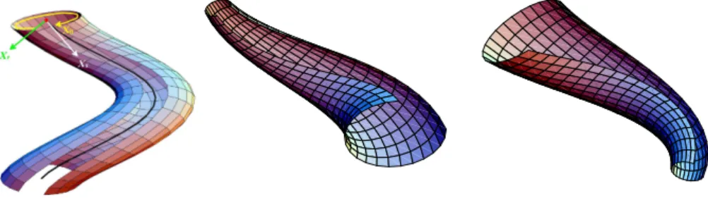
Curved surfaces strongly influence the flow dynamics be-cause transverse shearing and cross-stream momentum trans-port occur when the topography obstructs or redirects the motion due to curvature and torsion. Resistance due to basal friction is modified by “centrifugal forces” induced by bed curvature and torsion. The channel topography and the ge-ometry of the debris flow in the lateral and longitudinal di-rections are illustrated in Fig. 1. Similarly, Fig. 2 represents the geometric description of the coordinate system and some prototype channel geometries with uniform, diverging and converging curved and twisted channels that can be used in the transportation of granular materials. In what follows, ex-cept in Sect. 9.4, every quantity in this paper is written in non-dimensional form.
Pudasaini and Hutter (2003) extended the Savage-Hutter theory to flows of dry granular masses in a non-uniformly curved and twisted channel. First, we will outline the geo-metric configurations they implemented for dry granular flow that we will also adopt in this paper. Consider a debris flow-prone landscape and a subregion of it where the topogra-phy allows identification of the likely debris flow track. A space curve parallel to the thalweg of the valley is singled out as a master curve C (which can be obtained, e.g., by shifting the thalweg along its normal direction) from which the track topography will be modelled. The curvature and torsion of the master curve,κ=κ(x),τ=τ (x), are either as-sumed to be known or can be computed from digital elevation Geographic-Information-Systems (GIS) data as functions of the arc lengthx of the master curve. Then, an orthogonal coordinate system along the master curve is introduced; the model equations are derived in this general coordinate sys-tem. In the equations of this paper, (x, y) form a curved ref-erence surface, wherex is the coordinate along the thalweg of a mountain valley, whiley is the circular arc length in a cross-sectional plane perpendicular to the thalweg of which the value is determined by the relationy=εθ zT, whereεis
the aspect ratio between the debris flow height and extent,θ is the azimuthal angle which accounts for the cross-slope cur-vature andzT (usuallyzT≫1) is the radial distance between
the master curve and the thalweg andzis the coordinate per-pendicular to the reference topography.
T B
N(x) (x)
(x) O
O~
y
z
x talweg
master curve
ζ
θ
C ~
talweg
x
ζ
0~
x
lxr
Fig. 1.Left: The debris flow domain in the lateral direction occupies a region in a circular section of a plane perpendicular to the thalweg of the valley andθis the azimuthal angle in this plane.OO˜=zT is the radial distance between the master curve and the thalweg.{T,N,B}is
the moving orthonormal unit triad following the thalweg.ζ˜ is the slope angle of the thalweg with the horizontal. The depth of the avalanche in this section is represented by a height functionh(x, y, t)and is measured in the radial direction. Right: Debris flow passing through the transition into the run-out zone in a vertical plane containing the thalweg of the valley. In this picture,xlandxr are the left and right end
points of the continuous transition between the straight inclined upper part with inclination angleζ˜0and the horizontal run-out in the valley.
Fig. 2.Left: A representation of a curved and twisted channel, a reference curve and the tangent vectors along the coordinate lines. The dark line along the channel is the axis of the channel; following the notation of Fig. 1Xs∼T(x),Xr∼N(x),Xθ∼B(x). Middle: Diverging, and
Right: converging curved and twisted channels that can be used in the transportation of the granular and debris flow materials.
paper explicitly include curvature and torsion effects in a sys-tematic manner. This makes the extended model amenable to realistic debris motions down arbitrary guiding topographies. This can be accomplished by coordinate transformation. Dif-ferent from and extending the original SH-theory and all their previous extensions (e.g., Gray et al., 1999; Pudasaini et al., 2003) a moderately curved and twisted space curve is used to define an orthogonal curvilinear coordinate system. The governing balance laws of mass and momentum are written in these coordinates.
4 Governing equations for single-phase dry granular avalanche
If the interstitial fluid stressTfin (7) is zero then Eqs. (7) and
(8) together with the solid stress Eq. (9) and the boundary conditions of Sect. 2.3 describe the field equations for sin-gle phase avalanching motion. In this section we present the model equations for a single-phase dry granular avalanche.
Pudasaini and Hutter (2003) formulated the balance laws of mass and momentum as well as the boundary conditions in slope-fitted curvilinear coordinates of mountain surfaces,
non-dimensionalised the equations and averaged them over the depth of the avalanche. The final balance laws of mass, and momentum in the down-slope and cross-slope directions take the forms (correct toO(ε1+γ), 0<γ <1)
∂h ∂t +
∂
∂x(hu)+ ∂
∂y(hv)=0, (15) ∂
∂t (hu)+ ∂ ∂x
hu2+ ∂
∂y(huv)=hsx− ∂ ∂x
βxh2
2
!
, (16) ∂
∂t (hv)+ ∂
∂x(huv)+ ∂ ∂y
hv2=hsy−
∂ ∂y
βyh2
2
!
, (17) wherehis the depth of the avalanche measured normal to the reference surface and the factorsβxandβyare defined as
βx = −εgzKx, βy= −εgzKy. (18)
The termssx andsy represent, respectively, the net driving
accelerations in the down-slope and cross-slope directions and are given by
sx=gx−
u |u|tanδ
−gz+λκηu2
+εgz
∂b
∂x, (19) sy=gy−
v |u|tanδ
−gz+λκηu2
+εgz
∂b
in which |u|=√u2+v2 is the magnitude of the velocity field tangential to the reference (basal) topography and −gz+λκηu2is the normal stress at the bed.λκis the local
curvature of the thalweg, whilst
η=cos(θ+ϕ(x)+ϕ0) , (21) where ϕ(x)=−Rxx
0τ (x
′)dx′ gives the accumulation of the torsion of the thalweg from an initial positionx0 andϕ0is a constant. gx,gy andgz are the projected components of
the gravitational acceleration along the down-slope, cross-slope and normal directions of the channel, for explicit com-putation see, Pudasaini and Hutter (2003). The aspect ra-tio ε, and the measure of curvature relative to the typical debris flow length,λ, are both small numbers given by the scales[L],[H],[R]: ε=[H]/[L],λ=[L]/[R], that are used to non-dimensionalise the equations. Here,[L]is the typical avalanche length,[H]is the typical avalanche height and[R] is a typical radius of curvature of the channel. The basal to-pography (which is the elevation of the real toto-pography from the reference surfacez=0, and includes the small-scale ge-ometric features of the bed topography) will be denoted by z=b(x, y).
The first terms on the right-hand side of (19) and (20) are the gravitational accelerations in the down- and cross-slope directions, respectively. The second terms represent the dry Coulomb friction in which the normal tractions comprise of the overburden pressure(−gz)plus a contribution due to the
curvature and torsion of the master curve λκηu2
. Finally, the third terms are the projections of the topographic vari-ations along the normal direction. Kx and Ky in (18) are
called the earth pressure coefficients. Elementary geometri-cal arguments and Mohr’s circles may be used to determine these values as functions of the internal (φ) and basal (δ) an-gles of friction, (Hutter et al., 1993), viz.,
Kx =Kxact/pass=2 sec 2φ
1∓
q
1−cos2φsec2δ
−1, (∂u/∂x)≷0,
Ky =Kyact/pass= 1 2
Kx+1∓ q
(Kx−1)2+4 tan2δ
,
(∂v/∂y)≷0, (22)
whereKx andKy are active during dilatational motion
(up-per sign) and passive during compressional motion (lower sign). We note that ignoring theO(ε)-contributions in (15)– (20) reduces the equations to a mass point model and does not allow determination of the deformation of the pile. The dynamics of these equations will also be discussed in Sect. 6 in the context of debris flows. To describe the debris flow, this model must formally be altered only by adding the pore fluid stress.
5 Evolution and inclusion of the pore fluid stress
The evolution of the pore fluid stress is crucial in modelling debris flow phenomena. Here we will not present the en-tire calculation but only write the most important steps for
the inclusion of the fluid stress into the model equations of Sect. 4. The routine procedure for the coordinate transfor-mation, non-dimensionalisation, depth-integration, constitu-tive relations (for the solid phase) and assumption about the nearly uniform velocity profile through the debris flow depth can be found in Pudasaini and Hutter (2003). We will follow the spirit of their paper.
5.1 Contributions due to fluid stress
Using the orthogonal coordinates displayed in Figs. 1 and 2, and with a scaling and dimensional analysis as in Puda-saini and Hutter (2003) the new contributions due to the fluid stress (10) which we must add in the down-slope, cross-slope and normal components of the momentum balance equations of the single-phase dry granular material (see, Eqs. (4.5)– (4.7) in Pudasaini and Hutter, 2003) are, respectively
ε " ∂p ∂x− 2 NR
∂2u˜ ∂x2−
1 NR ∂ ∂y ∂ ˜ v ∂x+
∂u˜ ∂y
− 1
ε2N R
∂2u˜ ∂z2 #
+Oε1+γ,
(23) ε " ∂p ∂y− 2 NR
∂2v˜ ∂y2−
1 NR ∂ ∂x ∂ ˜ v ∂x+
∂u˜ ∂y
− 1
ε2N R
∂2v˜ ∂z2 #
+Oε1+γ,
(24) ∂p
∂z +O
ε1+γ. (25)
These are dimensionless local expressions andu,˜ v˜ are the local dimensionless velocity components along the down-slope and cross-down-slope directions, respectively,pis the dimen-sionless fluid pressure andNRis the quasi-Reynolds number
which is the fluid volume fraction weighted Reynolds num-ber (as introduced by Iverson and Denlinger, 2001) defined as
NR=
√ gL ρH νfµf
, (26)
wheregis the gravity acceleration,LandHare scales used in the non-dimensionalisation, the typical extent and height of the debris flow,νf is the volume fraction andµf the
vis-cosity of the fluid. A typical value ofNRis on the order of
105−106. In the derivation of (23)–(25), some simplifica-tions have been made, one being that the volume fraction of the fluid,νf is independent ofz. For complete list of these,
see Pudasaini and Hutter (2003). 5.2 Fluid pressure at the bed
granular flow (Eq. (4.7), Pudasaini and Hutter, 2003) we ob-tain the following equation for the pressure distribution in the mixture due to the solid and the fluid
∂p
∂z + ∂
∂z Ts(zz)
=gz−λκηu˜2+O (ε) . (27)
Integrating this from the surfacez=s(x, y, t )to the depthz, thereby settingu˜≃u+O(ε), yields
p+Ts(zz)=
−gz+λκηu2
(s−z)+O (ε) . (28) Therefore, the total pressure at the bed,z=b(x, y, t ), is pb+Ts(zz)b =−gz+λκηu2
h+O (ε) , (29) whereh(x, y, t )=s(x, y, t )−b(x, y, t )is the depth of the de-bris flow.
The fluid pressure is assumed to vary linearly through depth which is also consistent with (28) in the normal di-rection. The total stress on the bed is now decomposed into two parts, the fluid and solid pressures, as follows:
pb=3f
−gz+λκηu2
h+O (ε) , (30) Ts(zz)b = 1−3f
−gz+λκηu2
h+O (ε) , (31) corresponding to the fluid and solid phase pressures (see, e.g., Iverson and Denlinger, 2001; Hubbert and Rubey, 1959). Here, 3f ∈ (0,1) is a continuous parameter that
may depend on several factors such as the debris flow height, time and diffusion of the basal pore pressure along the mix-ture body from its front to tail. All these are functions ofx, y andt but not z. So, 3f6=3f(·, z). Moreover, the limit
3f=1 implies zero basal effective stress or complete
lique-faction (around the rear end of the debris body) and3f=0
for dry granular flow (e.g. in the vicinity of the front of the debris flow surge). This means that this parameter is mathe-matically analogous to the fluid volume fractionνf. In
ther-modynamic nonclassical solid-fluid-mixture theories separa-tions like (30) and (31) are referred to asimpositions of pres-sure equilibrium. They are one possible imposition, but other possibilities such as3pf,(1−3pf),p>0 are equally justified. The separation (30), (31) of the total stress is of constitutive nature and bears the advantages and disadvantages which all such equations exhibit. It is also evident from (30) that3f
is the ratio between the pore fluid pressure at the bed and the total normal pressure of the debris mass in the normal direc-tion. Measurements at the base of experimental flows show that coarse-grained surge fronts have little or no pore fluid pressure. In contrast, finer-grained thoroughly saturated de-bris behind surge fronts is nearly liquefied by high pore pres-sure (see Iverson, 1997; Iverson and Denlinger, 2001). So, parameterisation of3f is very crucial in the description of
the dynamics of debris flow surges. Needless to say that here as everywhere else grain size separation is neglected.
5.3 Modification of the friction law and earth pressure co-efficients
We must modify the Coulomb friction law and the earth pres-sure coefficient of the Mohr-Coulomb yield criterion accord-ing to the effect of the pore fluid pressure distribution. We identify the fluid normal stress as the pore fluid pressure. As before, we assume that the pore fluid pressure and the solids stressTs(zz)both vary linearly from their maxima at the base
to zero at the free surface of the flow. Equation (31) thus implies that the depth-averaged normal solid stress takes the form
Ts(zz)=12(1−3f) −gz+λκηu2
h+O (ε)
= −12gz(1−3f)h+O (ε
γ) . (32)
Note that, as in Pudasaini and Hutter (2003), λ=O(εγ), 0<γ <1 is assumed to have equations correct to O(ε1+γ). We further assume that the down-slope and cross-slope solid stresses vary linearly with the normal solid stress through the avalanche depth. This is achieved to leading order by the expressions
Ts(xx)=KxTs(zz)+O εγ
,
Ts(yy)=KyTs(zz)+O εγ. (33)
From (32) it follows that the depth-averaged down-slope and cross-slope solid stresses are given by
Ts(xx)= −12Kxgz 1−3fh+O (εγ) ,
Ts(yy)= −12Kygz 1−3fh+O (εγ) . (34)
This implies that the factorsβxandβyin (18) must be
mod-ified by the expression
βx = −εgzKx 1−3f, βy= −εgzKy 1−3f. (35)
Similarly, in (19)–(20) the normal solid stress at the bed −gz+λκηu2 must be replaced by (31) for the solid-fluid
mixture. Furthermore, the detailed basal topographic ef-fectsεgz∂b/∂xandεgz∂b/∂yin (19)–(20) must be replaced
by 1−3fεgz∂b/∂x and 1−3fεgz∂b/∂y, respectively
(see, Pudasaini and Hutter, 2003).
Finally, in order to distribute the topographic effects and gravitational driving forces to the solid and fluid components we decompose the components of gravitational accelerations as follows:
gx=gx(s)+gx(f )= 1−3fgx+3fgx,
gy=gy(s)+gy(f )= 1−3fgy+3fgy. (36)
Note that since we are using depth-integrated equations we do not need to decomposegz.
5.4 Depth integration
due to the fluid in the pores of the mixture material along the xandycoordinate directions, respectively
ε " ∂ ∂x
pbh/2+pb∂b ∂x − h NR ( 2∂ 2u
∂x2+ ∂2v ∂y∂x+
∂2u ∂y2−
3u ε2h2
)#
+Oε1+γ,
(37) ε " ∂ ∂y
pbh/2+pb∂b ∂y − h NR ( 2∂ 2v
∂y2+ ∂2u ∂x∂y+
∂2v ∂x2−
3v ε2h2
)#
+Oε1+γ,
(38) where pb is the fluid pressure at the bed defined by (30) whilstu, v are the depth-averaged velocity components in thexandydirections, respectively.
6 Model equations for two-phase debris flows
6.1 Initial boundary value problem
Incorporating all new effects emerging from the intersti-tial fluid and detailed by (23)–(38), the granular avalanche Eqs. (15)–(20) becomegeneralised model equations for two-phase mixture debris flowssliding and deforming down arbi-trarily curved and twisted channels. The governing equations read
∂h ∂t +
∂
∂x(hu)+ ∂
∂y(hv)=0, (39) ∂
∂t (hu)+ ∂ ∂x
hu2+ ∂
∂y(huv)=hsx− ∂ ∂x
βxh2
2
!
, (40)
∂ ∂t (hv)+
∂
∂x(huv)+ ∂ ∂y
hv2=hsy−
∂ ∂y
βyh2
2
!
, (41) which remain formally the same as those for single-phase dry granular avalanche, (15)–(17), but for two-phase debris flows with the following specifications
sx=sx(s)+sx(f ), sy=sy(s)+sy(f ), (42)
βx= −ε 1−3fgzKx, βy= −ε 1−3fgzKy, (43)
sx(s)= 1−3f
gx−
u |u|tanδ
−gz+λκηu2
+εgz
∂b ∂x
, (44)
sy(s)= 1−3f
gy−
v |u|tanδ
−gz+λκηu2
+εgz
∂b ∂y
, (45)
sx(f )=3fgx−ε
1 h ∂ ∂x
pbh
2 +p b h ∂b ∂x− 1 NR ( 2∂ 2u
∂x2+
∂2v ∂y∂x+
∂2u ∂y2−
3u ε2h2
)
,
(46)
sy(f )=3fgy−ε
1 h ∂ ∂y
pbh
2 +p b h ∂b ∂y− 1 NR ( 2∂ 2v
∂y2+
∂2u
∂x∂y+ ∂2v
∂x2−
3v ε2h2
) ,
(47)
in which Kx, Ky are given by (22). Note that, although
the basic solid-fluid mixture mass and momentum balance Eqs. (7) and (8) are not in conservative form, the final model equations presented here are in conservative form with source terms2. Dimensional analysis, depth integration and ordering processes made it possible to transform these equa-tions from non-conservative to conservative form.
Given the material parametersδandφand the elevation of the basal topography,b=b(x, y), above the curved reference surface, the viscosity and the volume fraction of the pore fluid, mixture density and fluid pressure distribution at the bed, Eqs. (39)–(47) allowh, uandvto be computed as func-tions of space and time, once appropriate initial and bound-ary conditions are prescribed.his the debris flow depth, and (u, v)are the depth-averaged velocity components parallel to the flow surface. As initial condition one commonly pre-scribes the geometry and velocity distributions of the debris flow at the initial time, usually for a mass at rest.
6.2 The physics of debris flow described by the present model equations
The model equations presented in this section represent var-ious physical properties of debris flows. We outline some of them as follows:
(i) By setting3f=0 and NR→∞(i.e., ignoring the
vis-cous terms), these model equations reduce to the ex-tended avalanche model equations of Pudasaini and Hutter (2003). On the other hand, when setting3f=1
(i.e., complete liquefaction at the bed and thus zero basal effective stress of the solid) these equations reduce to Boussinesq-type hydraulic (shallow-water) equations with a purely viscous dissipation, e.g., appropriate for a slurry. For intermediate cases the equations indicate a combination of Coulomb friction and viscous dissipa-tion that changes in response to the spatial and temporal changes of the pore pressure.
(ii) Due to the viscous fluid stress effects the equations con-tain viscous terms viasx(f )andsy(f ). Therefore, they
are no longer hyperbolic, but hyperbolic-parabolic; they degenerate into hyperbolic equations for single-phase avalanche flows of dry granular materials when the ef-fect of the pore fluid is ignored.
(iii) The model equations involve three non-dimensional parameters, viz., ε, λ and NR. (a) The first two
are purely geometric parameters and indicateno scale dependence. (b) In contrast, the third parameter, NR=ρH√gL/νfµf, serves as a dynamical scaling
factor that is analogous to the Reynolds number in New-tonian fluid. Therefore, the debris flow equations are 2Strictly speaking, the expressions within the square brackets in
scale-dependent. Moreover, if we adopt an advection-diffusion equation (see Sect. 9.4.2) as done by Iver-son and Denlinger (2001) for the determination ofpb (or 3f) then, a new parameter D, the so-called pore
pressure diffusivity, also enters into consideration as a new dynamical parameter. In computations, in order not to distort the geometry of the slide, we shall choose ε=λ=1 and thusL=H=R.
(iv) The order of different terms in (46) and (47) should be understood as follows. First, let us consider (46). Test simulations reveal that in debris flow dy-namics the effect of(2∂2u/∂x2+∂2v/∂y∂x+∂2u/∂y2) is negligible as compared to 3u/ε2h2. On the other hand, typically, NRε2 is of O(1). Therefore,
1 NR
2∂2u/∂x2+∂2v/∂y∂x+∂2u/∂y2−3u/ε2h2 is also ofO(1), consistent with the order of the other terms of (46). A similar analysis holds true for (47).
(v) For geophysical debris flows typical values ofεandNR
are 10−3and 106, respectively. We have already seen in single-phase avalanche equations that orderεterms must be retained in the final governing equations. This request is even more intensified for debris flow mod-elling. The lowest approximation (i.e.,O(1)) excludes the effect of the pore pressure, as is evident from (46), (47). Iverson and Denlinger (2001) have also concluded this fact.
(vi) An expression for the evolution of the basal pressure pbcan be obtained by an advection-diffusion equation forpbthat is responsible for the distribution of the pore
pressure along the bed of the debris flow. Iverson and Denlinger (2001) expressed 3f as a function of the
mixture height, time and the diffusivity of the mixture. Alternatively, Savage and Iverson (2003), coupled the pore pressure evolution equation with the mass and mo-mentum balance equation to describe debris flow surge dynamics over a one-dimensional rough incline. Here, first, we will take some constant values, and then a bilin-ear parameterisation of3f in time and space for
simu-lation. This simple parameterisation can also produce debris flow surges as discussed by Iverson and Den-linger (2001) and Savage and Iverson (2003). In ap-plications, one may couple these or other parameteri-sations or evolution equations for pore pressure of the fluid (as done in Sect. 9.4.2) with the present model equations to describe debris flow surges down more general mountain terrains.
(vii) The curvature, λκ, and torsion, η, effects of the ge-ometry enter in the model equations directly via the Coulomb friction terms in (44)–(45), but they are equally indirectly contained in the viscous terms (46)– (47) via the pressure, pb, at the bed, see (30). Note that the components of the gravitational accelerations gx,gy,gzalso include such effects due to the curvature
and torsion of the reference topography (see Pudasaini and Hutter, 2003).
7 The new features of the model equations
Equations (39)–(41) constitute atwo-dimensional conserva-tive system of equations which entails several advantages over previous model equations of the Savage-Hutter (1989) type for dry granular materials and Iverson (1997) type for mixtures. They are as follows:
(1) The equations systematically include the curvature and torsion of the channelised basal topography. They are written in a slope-fitted general orthogonal curvilinear coordinate system. Therefore, they can be utilised to describe debris flows along non-uniformly curved and twisted channels of general type.
(2) There is a non-zero gravity termgy in the cross-slope
direction, see (45) and (47), which takes into account the global effect of topographic variation in the lateral direction. Thus, the lateral motion is explicitly gravity driven, not only indirectly via lateral confinement gra-dient, i.e., ∂b/∂y. This might be crucial in designing defence structures and when debris flows hit obstruc-tions or are deflected on their ways. The torsion effect, ηof the topography is included in the net driving force componentssx andsy. The components of the
gravi-tational acceleration also depend on both the curvature and the torsion of the basal topography, (see Pudasaini and Hutter, 2003). They coordinate, which was just a straight line in the previous models, is now curved in the cross-slope direction and for a torsion-free master curve (i.e., η=1), which lies in a vertical plane, these model equations exactly degenerate to previous exten-sions (e.g., Gray et al., 1999).
(3) Similarly, these equations can exactly be reduced to the avalanche equations of Pudasaini and Hutter (2003) as special cases for which the parameters3f=0, NR→∞.
(4) We can form a three-dimensionally curved and twisted channel using down-slope and cross-slope coordinatesx andyalone. In principle, it is thus possible to model a given channel by considering its thalweg and by choos-ingθappropriately as a function of the down- and cross-slope coordinates. These are new flexibilities of the model equations which are crucial to describe the mo-tion of avalanching debris flows in curved and twisted channels and mountain terrains in a more realistic man-ner.
the parameter3f. Similarly, the structure of the
equa-tions shows that the granular avalanche equaequa-tions are of hyperbolic type whereas, due to the pore fluid dif-fusion, debris flow is governed by hyperbolic-parabolic type partial differential equations.
(6) In the present model the pore pressure at the bed,pb, includes effects of curvature and torsion of the bed to-pography, see (30). Numerical results show that such an effects are substantial, for detailed discussion, see Sect. 9.1 and Fig. 4.
(7) The coordinates of these model equations follow the basal topography. So, a mathematically correct asymp-totic analysis could rigorously be performed.
In this sense, one may infer that the above equations should be physically, geometrically and mathematically more suitable than previously proposed models (e.g., Iver-son, 1997; Iverson and Denlinger, 2001) for the description of debris flows down arbitrarily curved and twisted channels with variable cross-sections.
8 Numerical integration techniques
The debris flow equations (39)–(41) comprise a nonlinear conservation system. Shock formation, possibly diffusively smoothed out, is an essential mechanism in debris flows on an inclined surface merging into a horizontal run-out zone or encountering an obstacle when the velocity becomes subcrit-ical from its supercritsubcrit-ical state. Note that the formation of shocks in debris flow depends strongly on the volume frac-tion of the solid. Therefore, for high sediment concentra-tions debris flow surge fronts are most likely associated with a jump in the height and velocity field although the rear part of the debris is highly liquefied. This will be discussed in more detail in Sects. 9.3 and 9.4. To produce more accu-rate and physically reliable solutions of strongly convective nonlinear conservation equations, it is therefore natural to apply conservative high-resolution numerical techniques that are able to resolve the steep gradients of the unknown vari-ables and moving fronts often observed in experiments and field events of avalanches and debris flows. The NOC (Non-Oscillatory Central) scheme proposed first by Nessyahu and Tadmor (1990) and extended to higher dimensions by Jiang and Tadmor (1998) is implemented to solve the model equa-tions. This is a high resolution shock capturing scheme. The necessary background and full details of this method can be found in the literature (see, e.g., Harten, 1983; Harten et al., 1986; Yee, 1987; Nessyahu and Tadmor, 1990; LeVeque, 1990; Kr¨oner, 1997; Jiang and Tadmor, 1998; Toro, 2001) and its application to avalanches is, e.g., given by Tai et al. (2002), Pudasaini (2003), Pudasaini and Hutter (2003a), Wang et al. (2004) and Pudasaini et al. (2005a, b). We do not further elaborate here on the TVD (Total Variation Diminish-ing) techniques and optimal choices of limiters and cell re-constructions. Wang et al. (2004) made a careful study inves-tigating its optimal use in avalanche studies of the extended
Savage-Hutter equations. For alternative numerical schemes also see Denlinger and Iverson (2001, 2004), Koschdon and Sch¨afer (2003), Iverson et al. (2004), Patra et al. (2005) and Vollm¨oller (2004).
This scheme requires the system to be written in terms of conservative variables, which are the debris flow thickness, hand the depth integrated down- and cross-slope momenta, mx=huandmy=hv. With the vector of conservative
vari-ables, w=(h, mx, my)T, the model Eqs. (39)–(41) can be
written as ∂w
∂t + ∂f(w)
∂x + ∂g(w)
∂y =s(w). (48)
The down-slope and cross-slope momentum flux vectorsf andg, and the vector of the source termssare given by
f=
mx
m2x/ h+βxh2/2
mxmy/ h
,
g=
my
mxmy/ h
m2y/ h+βyh2/2
,
s=
0 hsx
hsy
. (49)
The terms βx andβy, defined in (43) incorporate the
ex-tending and contracting states of the avalanching debris mass through the active and passive earth pressures. Similarly, the source termssx andsy, described in (42), (44)–(47) are of
crucial importance as they include the total driving force gen-erated by gravity, friction, curvature, torsion and local details of the basal topography through its gradient terms and the pore pressure distribution of the viscous fluid. They jointly determine the dynamics of the flow.
9 Debris flow down curved and twisted channels
0 100 200 300 400 500 600 −100
−50 0 50 100
0 100 200 300 400 500 600
−100 −50 0 50 100
0 100 200 300 400 500 600
−100 −50 0 50 100 y
y
y
x
=
⇒
Λf = 0Λf = 0.2
Λf = 0.3 Upper Straight Part Transition Run-Out & Deposition Zone
t= 18 t= 38 t= 50 t= 70
t= 18 t= 38 t= 50 t= 70
t= 18 t= 38 t= 50 t= 70
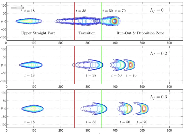
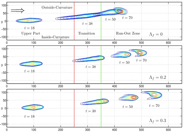
Fig. 3.Contour plots of an avalanching debris mass flowing down a curved chute that is flat in the lateral direction: granular-fluid mixture with fluid component:3f=0 (top),3f=0.2 (middle) and3f=0.3 (bottom). The upper part of the chute (x<250) is inclined at an angle of
45◦, the middle part is a transition zone (250<x<350) and the final part(x>350)is horizontal and flat. Time slices:t=18,38,50,70. The mass is initially kept in a hemi-spherical cap of radius 6.5 centred at(23,0)and initial velocity is zero. Internal and bed friction angles of the grains are 33◦and 27◦, respectively andNR=3×10⁵.All quantities are dimensionless.
new-model equations. On the other hand, they will open a wide spectrum of possibilities for practitioners involved in hazard mapping, risk management and public safety. For single-constituent dry granular avalanches, corresponding re-sults were obtained by Pudasaini et al. (2005a). This pa-per aims to extend those simulations for two-phase debris flows. In the sequel, we will separately present simulations (i)for a simply curved chute or a flume, and(ii)for contin-uously curved and twisted channels. We will consider dif-ferent (variable) volume fractions of the fluid component in order to study the explicit influence of the interstitial fluid in debris flow dynamics. Another important aspect of this paper is the coupling of the advection-diffusion equation, proposed by Iverson and Denlinger (2001) for the determination of the bed fluid pressure, with the model Eqs. (39)–(41), and com-parison of model simulations with the laboratory and field experiments.
9.1 Debris flows down a curved chute
Geometry of the chute and parameters:
Let us consider a chute with a flat upper part (x<250) inclined at an angle of 45◦, continuous transition zone (250<x<350) and a horizontal, flat, final part (x>350).
Only one curvature in the downhill direction is involved in this configuration. Hence, the chute is laterally flat and torsion-free, i.e.η=1.
Figure 3 depicts several contour plots of debris flows down such a curved chute in which the ratio between the pore fluid pressure at the bed and the total normal pressure of the debris mass perpendicular to it correspond to 3f=0
(top),3f=0.2 (middle) and3f=0.3 (bottom). For all
val-ues of 3f (roughly speaking, the volume fraction of the
fluid) the contours are plotted for four dimensionless time slices:t=18,38,50,70. The mass is initially kept in a hemi-spherical cap of radius 6.5 centred at(23,0)and the initial velocity is zero. The internal and bed friction angles of the grains are 33◦and 27◦, respectively, and the quasi-Reynolds number is taken to beNR=3×10⁵, see Iverson and Denlinger
(2001). These parameters will also be used in the remainder of the paper whenever applicable.
Discussion of results:
0 100 200 300 400 500 600 −100
−50 0 50 100
y
x
t= 18 t= 38 t= 50 t= 70
Λf = 0.3
Fig. 4.As in the last panel of Fig. 3 but neglecting the influence of the curvature in the pressure at the bed; manifesting substantial contribution of the term including the curvature in the dynamics of the debris flow.
in the transversal direction, see forms of the masses at time t=18 in all three panels in Fig. 3. This is clearly because the flow is driven by gravity. As soon as the mass enters the transition zone due to the longitudinal curvature of the chute, due to the increased friction the body starts extending also in the cross-slope direction. These effects are seen in all panels at timet=38. In the run-out zone the height of the pile is always increasing (fromt=50 tot=70) and the body comes to a rest, as plotted for timet=70. At all times the sliding and deforming debris body is symmetric about the central line (y=0) of the chute. This is evident because the chute is torsion-free.
Effects of the fluid:Our next aim is to study the influence of the fluid component in the dynamics of the debris flow. From the mechanism of the mixture of solid and fluid constituents it is clear that as the value of the parameter3f increases
the contribution of the fluid increases. This is simply due to the fact that the Coulomb friction between the grains is decreased, and that the debris mass is more liquefied. Con-sequently, with increasing values of the parameter 3f the
travel distance of the flow increases dramatically. The fluid presence also implies changes to the form of the body. The forms and positions of the fronts and tails and the curvature of the geometry of the deforming body are explicitly depen-dent on the value of3f. With increasing value of3f the
increase of the speed of the tail is much faster than the speed of the front (e.g., compare the three panels in Fig. 3 at time t=38). Further interesting phenomena are in the deposit and in the run-out zone. The top panel shows that the final deposit (timet=70) for dry granular flow is convex with its center ly-ing beforex=400, whilst for debris flow, e.g., with3f=0.3,
the center of the body lies beyondx=500, see the bottom panel; and the form of the deposit has reverse “Barchan dune type” geometry with two “horns” lying on either side of the central line of the chute facing the upstream direction.
From these observations one may draw the inferences that the form and speed of debris flows are explicitly influenced both by the geometry of the topography and the relative vol-ume fractions of the fluid and solid constituents in the mix-ture.
Effects of the curvature on the pressure at the bed
From Eqs. (30) and (31) one can infer that there is substan-tial contribution of the curvature and torsion on the pressure at the bed by the termλκηu2, hence on the flow dynamics. To see this effect quantitatively, we repeat the above simulation with3f=0.3, but without inclusion of the curvature in the
expression for the basal normal pressure, i.e.,pb=−3fgzh
andTs(zz)b =− 1−3fgzh. This shows that the pore fluid
pressure at the bed is decreased by the amount3f λκηu2
h but at the same time the solid (normal) pressure at the bed is also decreased by 1−3f
λκηu2h. This means that, al-though the mobility due to the fluid component is decreased (relatively) by 30%, the relative 70% decrease in the solid normal pressure reduces the Coulomb frictional resistance quite considerably, see (44) and (45), thus substantially in-creasing the reach of the debris body in the transition zone. Figure 4 displays the effect of the curvature on the pressure at the bed. Parameters chosen for the simulation are as in the last panel of Fig. 3, but the curvature of the bed topography is set to zero. The difference in the dynamics between these two pictures is substantial. Similarly, one can investigate the effect of the torsion on the pressure at the bed.
9.2 Debris flow down non-uniformly curved and twisted channels
At first, we consider helically curved and twisted channels. This is an academictest example, ahelixas a master curve so as to form a helically curved and twisted channel with other-wise circular and/or parabolic cross section. Let us consider a circular helix described by
R(ϑ )=(Acosϑ, Asinϑ,−Bϑ ) , (50) whereϑ is the azimuthal angle. The arc length, curvature, torsion and pitch of the helix are given by
x=A2+B2 1/2
ϑ,
κ =A/A2+B2,
τ = −B/A2+B2,
P =2π B, (51)
0 100 200 300 400 500 600 −100
−50 0 50 100
0 100 200 300 400 500 600
−100 −50 0 50 100
0 100 200 300 400 500 600
−100 −50 0 50 100 y
y
y
x
=
⇒
Λf = 0
Λf = 0.2
Λf = 0.3 Upper Part Transition Run-Out Zone
Inside-Curvature Outside-Curvature
t= 18
t= 38
t= 50
t= 70
t= 18
t= 38
t= 50
t= 70
t= 18
t= 38 t= 50 t= 70
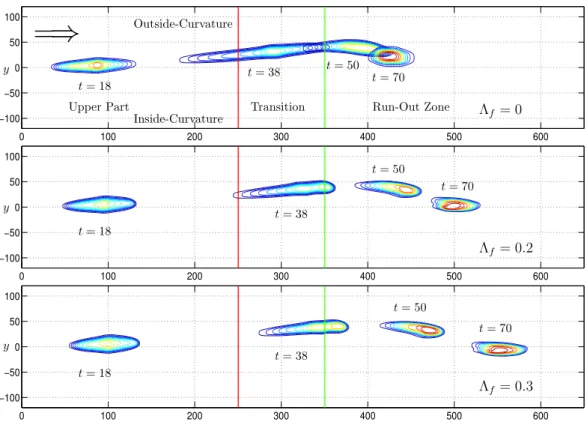
Fig. 5. Contour plots of avalanching debris mass flowing down a curved and twisted channel: granular-fluid mixture with fluid compo-nent: 3f=0 (top), 3f=0.2 (middle) and3f=0.3 (bottom). The upper part of the chute (x<250) is inclined at an angle of 45◦, the
middle part is a transition zone (250<x<350) and the final part(x>350)is a horizontal channel. Parameter values are: A0=B=300, y∈ [−120,120], zT=128. Time slices:t=18,38,50,70. The mass is initially kept in a hemi-spherical cap of radius 6.5 centred at(23,0)
and initial velocity is zero. Internal and bed friction angles of the grains are 33◦and 27◦, respectively andNR=3×10⁵.All quantities are
dimensionless.
Based on the master curve (50) a helically curved and twisted channel is formed. The lateral section of the topogra-phy is the intersection of a plane perpendicular to the thalweg of the channel and the channel itself. In the sequel, we will deal with cases in which the transition and run-out zones are included in the geometrical part of the model and that the cross-sectional geometry of the channel is also variable.
In reality channels may be arbitrarily curved and twisted with variable cross-slope curvature and channel width. Real-istic flow tracks go from steep to flat regions where the mov-ing masses come to a halt. The geometry must play a crucial role to make the body stand still. The concave curvature of the mountain side increases the bed friction and consequently forces the debris mass to slow down and eventually come to rest. In this subsection we will present debris flow simula-tions through more general channels which possess run-out zones.
9.2.1 Variable curvature and torsion
Consider a channel of which curvature and torsion are rede-fined with a new expression forAin (51) as follows:
A(x)=
A0, 0≤x ≤xl,
A0exp[(x−xl)a], xl≤x≤xr,
A0exp[(xr −xl)a], x ≥xr,
(52)
wherea determines the intensity of the decrease of the cur-vature and torsion. For the simulations, we have seta=1. Equation (52) tells us that the radius of curvature and torsion of the channel increase rapidly as the arc-lengthx becomes larger thanxl. Before this transition point, the channel has
uniform radius of curvature and torsion. This increase forces the channel quickly to merge (approximately) into a lesser and lesser curved and eventually horizontal channel. This horizontal portion of the channel also forms the run-out zone for the debris. There is a continuous decrease of the curva-ture and torsion fromxl=250 to xr=350. Then, forx≥xr
the curvature and torsion are always (almost) zero, and thus, the subsequent channel is forming a channelised circular run-out. The parameter values are:A0=300,B=300, so that the channel is inclined relative to the horizontal at 45◦. The ra-dius of curvature in the cross-slope direction iszT=128 and
y∈ [−120,120].
Discussion of results:
Geometric effects: Figure 5 displays thickness contours of debris flows with three different values of3f, respectively,
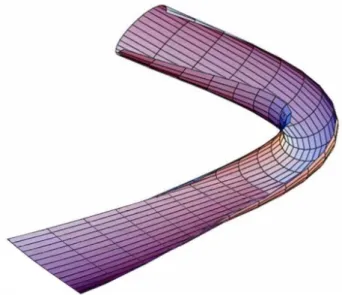
Fig. 6. Curved and twisted channel. The channel has a circular cross-section before the transition and merges continuously into the flat horizontal run-out zone.
(52) and a constant cross-slope channel width3. These con-tours are plotted at the time steps 18, 38, 50, 70, respectively. As time increases, the debris mass is laterally getting less spread, but, it is rapidly moving outwards from the center line of the channel in the front much more than in the back. This effect can clearly be seen in all three panels at timest=18 and t=38. This is so because the speed of the front is much larger than that of the tail. Such behaviour of the deforming mass is the joint effect of the curvature, torsion, and the radial accel-eration that is modelled in the theory (Eqs. (15)–(17) for dry avalanches, the top panel and Eqs. (39)–(41) for debris flows, the middle and bottom panels) through the gravitational ac-celeration componentsgx, gy, gz and the net driving force
componentssx,sy, which include the curvature and torsion
of the thalweg, bed topography and the cross-slope curvature of the channel.
Since the curvature and torsion of the channel are contin-uously decreasing for x>xl=250, from t=38 onward, the
debris mass tends to slow down and turn smoothly towards the central line of the channel due to the confinement gra-dient in the cross-slope. Corresponding to the decrease of the curvature and torsion, the inclination angle of the chute with the horizontal plane is also continuously decreased. Ultimately, the channel merges into a horizontal circularly curved channel, thus forming a gully-type channelised run-out zone. Somewhere in the transition zone the sidewise pressure (due to the lateral component of the gravitational 3All figures shown for helical chutes are geometrically distorted.
The graphs are vertical projections of the chute and debris heaps whose circular-annular geometry is stretched to become straight. Thus, a segment of the annular ring becomes a rectangle of which the top edge is the chute outside and the bottom edge the chute at the inside boundary. This graphical representation is chosen because it is relatively easy to program.
force towards the central line) from the channelised bed to-pography exceeds the force due to the radial acceleration. It leads to a continuous rotation of the body towards the center of the channel. This sidewise pressure is so strong that after x=350 the mass comes back to the thalweg of the channel (middle panel) and heads towards the opposite side of the channel (bottom panel). Finally, the body comes to rest at a time prior tot=70.
Effect of the fluid:The effect of the fluid is much more pro-nounced here than in the previous case with debris sliding over a curved but not twisted chute, see Fig. 3. With increas-ing value of the parameter3f the debris mass slides faster
throughout the channel and travels farther and farther in the run-out zone. Similarly, with the increasing value of3f the
center of mass of the final deposit comes closer and closer to the central line of the channel (compare top and middle pan-els) and ultimately it crosses the central line (bottom panel). This behaviour of the motion of the body is dominated by both the geometry of the channel and the contribution of the fluid component in the mixture. Since the chute is uni-formly channelised from initiation to the run-out zone in the cross-section the mass can not spread in the lateral direction not even in the run-out zone. Instead, it is accumulated and elongated around and along the thalweg of the channel. The channelised topography also does not allow the formation of the Barchan type geometry of the debris mass in the run-out zone.
9.2.2 Decreasing curvature & torsion, and variable cross-slope curvature
Real channels may be diverging or converging (with respect to their channel width or cross-slope curvature) along the downhill direction, see Fig. 2. Therefore, the debris flow theory must be able to deal with more general channels with varying cross-slope curvature. At this point, we simulate the debris flow motion in a channel of which the parameterAis defined by (52) as in the previous case, but, now we vary the channel width starting from its left boundary of the transi-tion zone. This case is more important in geophysical appli-cations because curvature and torsion decrease as one enters into the horizontal run-out zone of a mountain valley. This effect can be achieved by defining a channel which merges continuously into an open flat run-out zone according to
θ (x, y)=
y/zT, 0≤x≤xl,
(y/zT)f (x), xl ≤x ≤xr,
0◦, x≥xr,
(53)
where zT is the distance between the master curve and the
thalweg in the upper inclined part of the channel (hence a constant) andf (x)=(1−(x−xl) / (xr−xl))2. Thus, the
con-tinuous transition of the parametric functionθfrom its higher value (y/zT) in the upper part to its zero value in the open
0 100 200 300 400 500 600 −100
−50 0 50 100
0 100 200 300 400 500 600
−100 −50 0 50 100
0 100 200 300 400 500 600
−100 −50 0 50 100 y
y
y
x
=
⇒
Λf = 0
Λf = 0.2
Λf = 0.3 Upper Part Transition Run-Out Zone
Inside-Curvature Outside-Curvature
t= 18
t= 38
t= 50 t= 70
t= 18
t= 38
t= 50 t= 70
t= 18
t= 38
t= 50 t= 70
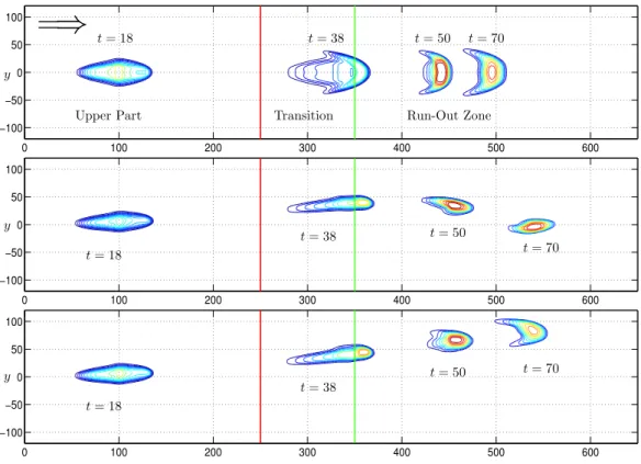
Fig. 7.Contour plots of avalanching debris flowing down a curved and twisted channel: granular-fluid mixture with fluid component:3f=0
(top),3f=0.2 (middle) and3f=0.3 (bottom). The upper part of the chute (x<250) is inclined at an angle of 45◦, the middle part is a
transition zone (250<x<350) and the final part(x>350)is horizontal and flat. Parameter values are:B=300,Ais redefined withA0=300, the channel width is redefined with variableθ,y ∈ [−120,120],zT=128. Time slices: t=18,38,50,70. The mass is initially kept in a hemi-spherical cap of radius 6.5 centred at(23,0)and initial velocity is zero. Internal and bed friction angles of the grains are 33◦and 27◦, respectively andNR=3×10⁵.All quantities are dimensionless.
Discussion of results:
Geometric effects: Figure 7 depicts the contours of the de-bris flow motion after its release to the open run-out zone. The graphs describe the deformation of the debris disclos-ing the subtle reaction of it to the different geometry of the transition and run-out region. Although the inclination of the channel is decreasing after reaching the transition zone, the debris body is heading radially outwards of the flat run-out zone until it comes to rest close to the outside edge of the open channel. The main mechanism for this is that, as soon as the mass enters the runout zone the radial acceleration de-creases rapidly, but, since the chute is flattening in the cross-slope direction, after the transition zone, the material body moves in the direction of the velocity at the moment directly after the transition, departing away from the central line, and the velocity is decreasing with time due to the bed friction until the debris body comes to rest. The direction and the process of the deposition is in conformity with our physical intuition and expectation.
Effects of the fluid: The most interesting effect of the fluid component can be observed in this figure. Before the tran-sition zone, the dynamics of the flow is exactly the same as in Fig. 5, travel distances in the run-out zones are also
sim-ilar. But, the form of the sliding body in the run-out zone is completely different from that for the entirely channelised topography (Fig. 5). Since the channel is gradually opened in the run-out zone the radial acceleration makes it possible to form the Barchan type geometry as in Figs. 3 and 4, but now with the horns pointing obliquely-upstream. Note that with increasing value of the fluid component the aerial coverage of the deposit is also increasing.
9.3 Variable pore pressure distribution
A simple parameterisation for pore fluid pressure. The structure of Eqs. (39)–(47) indicates that3f plays a
signif-icant role in the description of the debris flow (see, Iverson and Denlinger, 2001; Savage and Iverson, 2003 for further explanation). Therefore, a proper parameterisation or de-scription of3f is necessary. In reality, the pore-fluid
pres-sure is not constant but varies with time and along the debris body, usually its value being smaller in the front and larger in the rear part. As a first attempt, to investigate the effect of the variable pore pressure to the dynamics of debris flow we parameterise3f as
3f =3meanf −13f
x−(xr +xf)/2
xf −xr
(t−t0) (tmax−t0)
0 100 200 300 400 500 600 −100
−50 0 50 100
0 100 200 300 400 500 600
−100 −50 0 50 100
0 100 200 300 400 500 600
−100 −50 0 50 100 y
y
y
x
=
⇒
Upper Part Transition Run-Out Zone
t= 18
t= 38
t= 50 t= 70
t= 18
t= 38 t= 50
t= 70
t= 18 t= 38 t= 50 t= 70
Fig. 8. Contour plots of avalanching debris flowing down curved and twisted channels: granular-fluid mixture with variable pore fluid pressure that varies (increases) linearly from the front to the tail side of the debris body. Top, middle and bottom panels correspond to bottom panels of Figs. 3, 5 and 7, respectively, that were plotted for constant pore fluid pressure throughout the body. The upper part of the chute (x<250) is inclined at an angle of 45◦, the middle part is a transition zone (250<x<350) and the final part(x>350)is the run-out zone. Time slices:t=18,38,50,70. The mass is initially kept in a hemi-spherical cap of radius 6.5 centred at(23,0)and initial velocity is zero. Internal and bed friction angles of the grains are 33◦and 27◦, respectively andNR=3×10⁵.
where,3meanf is the mean value of3f in the longitudinal
di-rection between its front and rear values,13f the difference
of3f at the rear end and the front of the body for the final
time,t0the initial time andtmaxthe maximum time for nu-merical computation. For the simulation we take3meanf =0.3 and13f=0.3. So,3f is a bilinear function of space and
time with its largest value at the rear and smallest value at the front of the debris body. When t=tmax the maximum value of3f at the rear end is 50% larger (i.e., 0.45), and at
the front 50% smaller (i.e., 0.15) than its value at the center (i.e., 0.3) of the body. Equation (54) thus describes a simple mechanism for the diffusion of the pore fluid pressure from the rear to the front of the debris body.
Effects of variable pore fluid pressure. Figure 8 depicts three panels for the debris flow simulation over the simply curved chute (top), the curved and twisted channel with uni-form cross-section from initiation to the deposit (middle), and the curved and twisted channel with open flat run-out zone (bottom), corresponding to the last panels of Figs. 3, 5 and 7, respectively. In these simulations the other parameters are as before, but with variable pore pressure distribution as parameterised by (54). Compared with their previous coun-terparts, one observes two significant influences of the vari-able pore pressure at the bed, (i) in the forms of the debris
flow surges, and (ii) out distances, mainly in the run-out zones. In each case, it is seen that the fronts move a bit slower and the rears move faster than those for constant pore pressure distribution. The reason for this is the decreasing bed friction angle as one moves towards the tail of the body from its front. Another interesting effect is seen around the front of the body, where the surface gradient increases with increasing time and increasing value of the fluid component (compare the graphs in all three panels fort≥38). Similarly, the travel distances of debris bodies are also shorter than be-fore. These phenomena can be explained somehow with ref-erence to observations. Measurements at the base of experi-mental flows show that coarse-grained surge fronts have little or no pore fluid pressure. In contrast, the finer-grained thor-oughly saturated debris behind surge fronts is highly lique-fied by high pore pressure (Iverson and Denlinger, 2001). As we will see, the present model, when coupled with a reason-able pore pressure distribution which may be determined by an appropriately postulated equation, is able to address these problems.
9.4 Comparison with experiments