Hydrological and meteorological investigations in a periglacial lake catchment near Kangerlussuaq, west Greenland – presentation of a new multi-parameter dataset

(1)

ESSDD

7, 713–756, 2014

Hydrological and meteorological investigations in a periglacial lake

catchment

E. Johansson et al.

Title Page

Abstract Instruments

Data Provenance & Structure

Tables Figures

◭ ◮

Back Close

Full Screen / Esc

Printer-friendly Version

Interactive Discussion

Discussion

P

a

per

|

Discussion

P

a

per

|

Discussion

P

a

per

|

Discussion

P

a

per

|

Earth Syst. Sci. Data Discuss., 7, 713–756, 2014 www.earth-syst-sci-data-discuss.net/7/713/2014/ doi:10.5194/essdd-7-713-2014

This discussion paper is/has been under review for the journal Earth System Science Data (ESSD). Please refer to the corresponding final paper in ESSD if available.

Hydrological and meteorological

investigations in a periglacial lake

catchment near Kangerlussuaq, west

Greenland – presentation of a new

multi-parameter dataset

E. Johansson1,2, S. Berglund4, T. Lindborg2,3, J. Petrone2, D. van As5, L.-G. Gustafsson6, J.-O. Näslund1,2, and H. Laudon3

1

Department of Physical Geography and Quaternary Geology, Bert Bolin Centre for Climate Research, Stockholm University, 106 91, Stockholm, Sweden

2

Swedish Nuclear Fuel and Waste Management Co, Box 250, 101 24, Stockholm, Sweden

3

Department of forest ecology and management, Swedish University of Agricultural science, 90183 Umeå, Sweden

4

Hydroresearch AB, St. Marknadsvägen 15S (12th floor), 18334, Täby, Sweden

5

Geological Survey of Denmark and Greenland (GEUS), Øster Voldgade 10, 1350 Copenhagen, Denmark

6

(2)

ESSDD

7, 713–756, 2014

catchment

E. Johansson et al.

Title Page

Tables Figures

◭ ◮

Back Close

Full Screen / Esc

Discussion

P

a

per

|

Discussion

P

a

per

|

Discussion

P

a

per

|

Discussion

P

a

per

|

Received: 15 October 2014 – Accepted: 27 October 2014 – Published: 16 December 2014 Correspondence to: E. Johansson (emma.johansson@skb.se)

(3)

ESSDD

7, 713–756, 2014

catchment

E. Johansson et al.

Title Page

Tables Figures

◭ ◮

Back Close

Full Screen / Esc

Discussion

P

a

per

|

Discussion

P

a

per

|

Discussion

P

a

per

|

Discussion

P

a

per

|

Abstract

Few hydrological studies have been made in Greenland, other than on glacial hydrology associated with the ice sheet. Understanding permafrost hydrology and hydroclimatic change and variability, however, provides key information for understanding climate

change e_ffects and feedbacks in the Arctic landscape. This paper presents a new

ex-5

tensive and detailed hydrological and meteorological open access dataset, with high

temporal resolution from a 1.56 km2 permafrost catchment with a lake underlain by

a through talik close to the ice sheet in the Kangerlussuaq region, western Green-land. The paper describes the hydrological site investigations and utilized equipment, as well as the data collection and processing. The investigations were performed be-10

tween 2010 and 2013. The high spatial resolution, within the investigated area, of the dataset makes it highly suitable for various detailed hydrological and ecological studies on catchment scale. The dataset is availble for all users via the PANGAEA database, http://doi.pangaea.de/10.1594/PANGAEA.836178. Please note this dataset is under review and recommended not to be used before the final version of the manuscript is 15

accepted for publication.

1 Introduction

Future climate change is expected to be most pronounced in the Arctic region (Kattsov et al., 2005) and the terrestrial and aquatic ecosystems in the Arctic are predicted to undergo fundamental changes the coming century (Vaughan et al., 2013). To en-20

able predictions of the ecological response to changes in the hydrological and biogeo-chemical cycles, the understanding and prediction of these responses on the land-scape scale has to be improved (Rowland et al., 2010). Hydrology is the key driver for transport of matter within and between ecosystems. To describe the potential future impact on periglacial areas related to changes in the hydrological cycle in the Arc-25

(4)

sum-ESSDD

7, 713–756, 2014

catchment

E. Johansson et al.

Title Page

Tables Figures

◭ ◮

Back Close

Full Screen / Esc

Discussion

P

a

per

|

Discussion

P

a

per

|

Discussion

P

a

per

|

Discussion

P

a

per

|

marises the present knowledge on permafrost hydrology and in Kane and Yang (2004) waterbalances from 39 Arctic catchments are presented. However, only few hydrologi-cal data sets from Arctic regions exist containing necessary information on both surface and subsurface waters within the same catchment. This is due to the inaccessibility of

these remote areas and the harsh climatic conditions, but is also an e_ffect of the

rela-5

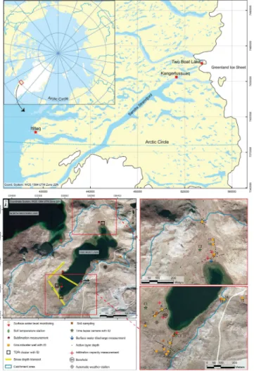
tively short period of the year when unfrozen water is present and can be monitored. In this work, we present hydrological data obtained from a detailed site investigation performed within the framework of the Greenland Analogue Surface Project (GRASP). The study area, here referred to as the Two Boat Lake (TBL) catchment, is located close to the Greenland Ice Sheet in the Kangerlussuaq region, western Greenland 10

(Fig. 1). The investigations were initiated in 2010, and have resulted in a wealth of in-formation on hydrology, meteorology, geometry (surface topography, lake bathymethry, and regolith and active layer depths), properties and spatial distributions of vegetation and soils, hydrochemistry, soil temperature, and geochemical processes and properties of the limnic and terrestrial ecosystems within the catchment. The aim of the GRASP 15

project is two-fold. The first part focused on how ecosystems develop and react in a long-term climate change perspective during an entire glacial cycle (Lindborg et al., 2013). The other part aimed at improving the understanding of water exchanges be-tween surface water and groundwater in a periglacial environment (Bosson et al., 2012, 2013).

20

The objective of the present paper is to describe the hydrological and meteorological installations and measurements in the TBL catchment, and to make the dataset avail-able to the scientific community. The aim of the hydrological field studies presented here was to quantify and identify the main hydrological processes in a periglacial lake catchment, thereby providing input to conceptual and mathematical modelling. In com-25

(5)

ESSDD

7, 713–756, 2014

catchment

E. Johansson et al.

Title Page

Tables Figures

◭ ◮

Back Close

Full Screen / Esc

Discussion

P

a

per

|

Discussion

P

a

per

|

Discussion

P

a

per

|

Discussion

P

a

per

|

2 Site description

The Kangerlussuaq region, comprising a hilly tundra landscape with numerous lakes, is the most extensive ice free part of Greenland. Continuous permafrost interrupted by through taliks under larger lakes covers the area. A permafrost depth greater than 300 m has been observed from temperature measurements in deep bedrock boreholes 5

∼5–6 km from TBL (Harper et al., 2011). An active layer of 0.15–5 m, depending on

soil type and vegetation cover, overlie the permafrost in the area from the settlement of Kangerlussuaq up to the ice sheet margin (van Tatenhove and Olesen, 1994).

The regional climate is dry with a mean annual precipitation of 149 mm in Kanger-lussuaq (uncorrected data, see Sect. 4.1) and with a mean annual air tempera-10

ture of ₋5.1◦_{C (measured 1977–2011; Cappelen, 2014). Discharge measurements}

in the Watson River, which is the main river in the area, were performed in

Kanger-lussuaq during the period 2007–2013 with an average annual cumulative runoff of

370 mm year−1 _{(Hasholt et al., 2013). This is almost entirely melt water from the ice}

sheet, since 94 % of the Watson River drainage area is glaciated. No rivers outside 15

the melt water system are present in the area. Mostly small intermittent streams (often formed by ice wedges) transport surface water to the many lakes in the area. Many outlet streams of precipitation driven lakes dry out during the main part of the year due to low precipitation. The low precipitation is also manifested through the relatively large amount of saline lakes in the area (Hasholt and Anderson, 2003). This means 20

that two main types of hydrological regimes in lakes can be identified in the area; lakes not in contact with the melt water system driven by precipitation and lakes receiving

water mainly from ice sheet melting. The TBL catchment with an area of 1.56 km2and

lake coverage of 24 %, is a precipitation-driven lake situated approximately 500 m from the Greenland ice sheet and 25 km north east of Kangerlussuaq (Fig. 1). The stream 25

in the outlet (Fig. 1) of the lake connects to the proglacial water system from the ice sheet, but no inflow of ice sheet melt water occurs. The catchment boundaries and

(6)

ESSDD

7, 713–756, 2014

catchment

E. Johansson et al.

Title Page

Tables Figures

◭ ◮

Back Close

Full Screen / Esc

Discussion

P

a

per

|

Discussion

P

a

per

|

Discussion

P

a

per

|

Discussion

P

a

per

|

based on LiDAR measurments in the terrestrial parts of the catchment and eco sound-ing investigations in the lake. The lake is underlain by a through talik, an observation

based on temperature data from a 225 m long borehole drilled in a 60◦inclination under

the TBL (Harper et al., 2011). The mean temperature at 140 m depth in the bedrock

under the lake was 1.25◦_{C and there are no indications of decreasing temperatures}

5

in the deepest part of the borehole, which would have indicated a closed talik (Harper et al., 2011). This interpreted through talik provides a possibility of hydrological con-tact between the lake surface water and the deep unfrozen groundwater system below the permafrost. There are several similar sized, and larger, lakes in the area (Fig. 1), many of which likely also maintain through taliks. Thus TBL is probably hydraulically 10

connected with other lakes in the region via taliks and perhaps also with unfrozen parts of the sub glacial areas.

Till and glaciofluvial deposits dominate the regolith in the TBL catchment (Clarhäll, 2011) and have a general depth ranging from 7–12 m in the valleys to zero on the hill sides where bedrock outcrops dominate. Petrone (2013) made radar observations 15

of an eolian silt layer of a thickness up to 1.5 m in the TBL catchment, underlain by

an ∼10 m thick till layer. The vegetation in the TBL catchment area is dominated by

dwarf-shrub heath (Clarhäll, 2011).

The TBL site is accessible via a road from the Kangerlussuaq international airport, which makes the site relatively easily reachable compared to most other Arctic loca-20

tions. The relatively small catchment, enabling a detailed spatial coverage of mea-surements of catchment processes, in combination with the fact that the hydrological system is not directly influenced by melt water from the ice sheet were the main rea-sons for selecting the TBL catchment as a case study area for periglacial hydrology and ecology.

(7)

ESSDD

7, 713–756, 2014

catchment

E. Johansson et al.

Title Page

Tables Figures

◭ ◮

Back Close

Full Screen / Esc

Discussion

P

a

per

|

Discussion

P

a

per

|

Discussion

P

a

per

|

Discussion

P

a

per

|

3 Installations and measurements

3.1 Strategy

Besides the scientific questions to be answered, the measurement program was to large extent determined by what was possible, given the hydrologic, climatic and logis-tic conditions at the site. Due to its remote location, but also depending on the harsh 5

climate, the site has been manned only during relatively short periods. This limited the possibilities for long-term or continuous observations of some parameters that could not be measured automatically (e.g surface water inflow to the lake or groundwater monitoring in the active layer). Lack of infrastructure for electrical power and telecom-munications has also been a limiting factor.

10

Hydrological processes and conditions not considered in temperate climate regions may be of great importance in periglacial areas. Hydrological responses in these cold

areas di_ffer in fundamental aspects from catchments in boreal and temperate regions

(Kane and Yan, 2004). Most importantly, the hydrology in periglacial environments is intimately connected to the presence of permafrost (White et al., 2007) and the active 15

layer dynamics. Snow related processes (wind drift of snow and sublimation) have also been shown to be of great importance for the annual water balance (Reba et al., 2012; McDonald et al., 2010). The overarching target when planning the TBL field programme was to identify and quantify the main hydrological processes including the interactions between surface water (in the lake and in the surrounding catchment) and the role 20

of both supra- and sub-permafrost groundwater. The dry climate and the very limited

surface water runo_ffin the area imply that conventional discharge measurements are

not meaningful; such measurements are otherwise a cornerstone in water balance studies (e.g. Johansson, 2008; Bosson et al., 2010). Hydrological processes and major

events on di_fferent spatial scales have been captured by time lapse cameras installed

25

(8)

ESSDD

7, 713–756, 2014

catchment

E. Johansson et al.

Title Page

Tables Figures

◭ ◮

Back Close

Full Screen / Esc

Discussion

P

a

per

|

Discussion

P

a

per

|

Discussion

P

a

per

|

Discussion

P

a

per

|

hydrological investigations together with a monitoring programme for soil water content, soil temperatures, groundwater levels in the active layer and lake surface water levels. Data from all monitoring equipment, except from the AWS, were collected manually during field campaigns, either by manual measurements or by retrieving data from loggers. Typically three field campaigns per year have been organized during the period 5

for which data are presented.

3.2 Meteorological data time series

The AWS, labelled KAN_B, was installed at a 70 m distance from the lake on 13 April 2011 (Fig. 2). The station is similar to approximately 20 other AWS installed on the ice sheet within the framework of the Programme for Monitoring of the Green-10

land Ice Sheet (PROMICE) (Van As et al., 2011), of which another three are located in the Kangerlussuaq region (Van As et al., 2012). The station at TBL measures air

temperature (∼2.55 m above ground), air pressure, humidity (∼2.55 m above ground),

wind speed and direction (∼3.05 m above ground), and the downward and upward

components of shortwave (solar) and longwave (terrestrial) radiation. A sonic ranger 15

was mounted on the AWS to register changes in surface level due to the presence of snow. All variables were recorded every ten minutes and processed to provide hourly averages. Values were stored locally, and hourly and daily averages were transmitted via satellite in summer and winter, respectively. Details about the instrumentation are given on http://www.promice.org.

20

An important addition to the station, compared to the PROMICE stations located on the ice sheet, is a precipitation gauge capturing both snow and rain. The snow is melted in the gauge and the Snow Water Equivalent (SWE) is measured. A Geonor T-200B was used (http://www.geonor.com/brochures/t-200b-series-all-weather.pdf), which weighs the precipitation in a 12 L bucket using a precision load cell with a vibrat-25

(9)

ESSDD

7, 713–756, 2014

catchment

E. Johansson et al.

Title Page

Tables Figures

◭ ◮

Back Close

Full Screen / Esc

Discussion

P

a

per

|

Discussion

P

a

per

|

Discussion

P

a

per

|

Discussion

P

a

per

|

Maintenence of the AWS occured once a year and entailed reading out the high tem-poral resolution data from the logger, and replacing sensors for recalibration. On every visit, the liquid content of the precipitation gauge was removed before a replacement mixture of ethylene glycol and methanol was added.

3.3 Sublimation and evaporation 5

Observations in the TBL area show that the snow cover decreased also during some periods of freezing temperatures, especially during clear windy days in late winter. This indicates that sublimation could be a process of importance. Therefore, sublimation measurements were performed at three sites within the catchment (Fig. 1) during three clear and sunny days in April 2013. Even though measurements were performed during 10

a short time period, they are judged to give a good estimation of the potential mass loss

via snow sublimation. For each site, 5 white pans (0.34 m_×0.22 m_×0.045 m) were filled

with snow and the weight of each box was noted. The mass loss was measured every 24 h with a precision scale in order to estimate the sublimation rate.

The same basic methodology was used when measuring evaporation in Au-15

gust 2013, i.e the same pans were placed at the same sites during three days in August and the mass loss was measured. Specifically the boxes were filled with water and the mass loss due to evaporation was measured every day. No rain or snow was observed during the measuring period which was characterized by variable clear and cloudy skies.

20

3.4 Snow depth and snow water content

The snow depth and associated snow water content were manually measured in April 2011. The catchment was sub-divided into four domains: (i) areas without snow cover, (ii) intermediate areas with snow cover broken up by spots without snow in uphill areas and on steepslopes, (iii) valleys with snow cover, and (iv) the lake ice. Based on 25

(10)

ESSDD

7, 713–756, 2014

catchment

E. Johansson et al.

Title Page

Tables Figures

◭ ◮

Back Close

Full Screen / Esc

Discussion

P

a

per

|

Discussion

P

a

per

|

Discussion

P

a

per

|

Discussion

P

a

per

|

domain type (i) (the transects are shown in Fig. 1). The snow depth was measured every five meters along all transects. At every fifth depth location, snow samples were collected using a standardized snowtube sampler with an inner diameter of 4.5 cm. The snow samples were weighed in the field using a portable scale. The correspond-ing snow water contents were calculated uscorrespond-ing the known sample volumes.

5

3.5 Water levels and discharge

Surface water levels were monitored using pressure transducers placed at the lake bottom both in TBL and in the lake located west of TBL (Fig. 1). The north-western lake, which is located at an elevation approximately 19 m above the TBL water level, is monitored with the purpose to get a reference lake level fluctuation in the area. 10

This is also a precipitation driven lake but belongs to a different surface water system

and discharges into a lake situated south of TBL. Details of equipment and measuring period are given in Table 1a. The transducers were placed at a minimum depth of 5 m to avoid disturbance from ice during the winter. A steel wire connected each transducer to the shore where it was firmly attached. Total pressure (hydrostatic and barometric) 15

and temperature were logged every third hour.

The shallow active layer depth in combination with the dry climate results in unsatu-rated conditions in most of the active layer. This makes monitoring of groundwater lev-els complicated. Fifteen groundwater wells (of type PEH50, with inner diameter 41 mm) were installed in the catchment to enable groundwater level monitoring and sampling. 20

The groundwater wells were primarily installed in local discharge areas along the val-leys floor (Fig. 1) in order to maximize the possibility to get the required volumes of water for chemical analyses.

The wells, consisiting of a bottom plug and a fully screened pipe section, were in-stalled with the bottom plug reaching the permafrost surface; the bottom plugs typically 25

(11)

ESSDD

7, 713–756, 2014

catchment

E. Johansson et al.

Title Page

Tables Figures

◭ ◮

Back Close

Full Screen / Esc

Discussion

P

a

per

|

Discussion

P

a

per

|

Discussion

P

a

per

|

Discussion

P

a

per

|

visits and in the summer of 2013 the groundwater levels were automatically monitored by pressure transducers in ten of the fifteen wells (Table 2). The pressure transducers cannot handle frozen water so the equipment was removed in the autumn.

Due to the very restricted amount of running water, no permanent discharge stations measuring surface water inflows to or outflows from the lake were installed. Instead, 5

a simple temporary installation was used to measure intermittent flowing surface water into TBL led through a PVC-pipe at the outlet of one of the main sub-catchment of the area where running water has been visible during wet periods. This small brook, shaped by ice wedges, dewatered the main part of the northern valley (Fig. 1). Manual measurements of this surface water inflow to the lake were made when field crew was 10

present at the site in June and August–September 2013. Even though the total inflow to the lake was not captured in these measurements, they provided data supporting the development of the conceptual understanding of the site hydrology. In particular, the response to rain events and the magnitude of base- and peak flow components could be analysed. No surface water outflow has occurred from the lake since the project 15

started, i.e during the period 2010–2013, which means that no such measurements have been possible.

3.6 Soil water content

Spatial and temporal variations of soil water content were monitored by use of the Time Domain Reflectometry technique (TDR, Stein and Kane, 1983), details about the 20

equipment are given in Table 1. In September 2011, 43 TDR-sensors were installed in three clusters, here referred to as Cluster 1–3, within the catchment (Figs. 1 and 3). Each cluster consists of a number of depth profiles where TDR sensors were placed so that they cover the whole interval from just below the ground surface to the permafrost surface that constituted the bottom of the active layer at the time of installation. Clusters 25

(12)

ESSDD

7, 713–756, 2014

catchment

E. Johansson et al.

Title Page

Tables Figures

◭ ◮

Back Close

Full Screen / Esc

Discussion

P

a

per

|

Discussion

P

a

per

|

Discussion

P

a

per

|

Discussion

P

a

per

|

four sensors, which were placed along a transect from the lake into the catchment

(Fig. 3c). The di_fferent clusters were arranged so that they form transects both along

and transverse to the dominating flow direction (Fig. 3a), which generally was judged to be perpendicular to the lake shoreline.

The depth profiles of TDR sensors were installed in pits (one pit per profile) that 5

were dug down to the distinct permafrost surface. Four TDR sensors were installed, with more or less constant distance between the sensors, so that it covered the en-tire depth in each particular pit. All TDR sensors in a cluster were connected to a central unit, consisting of a data logger, an electrical power central and an earth spike. A table describing the depth and ID-code of each TDR-sensor is available via 10

http://doi.pangaea.de/10.1594/PANGAEA.836178.

3.7 Hydraulic properties of the soil in the active layer

3.7.1 Sampling

Undisturbed soil samples were collected, at four di_fferent depths, in metal cylinders

for analyses of soil water retention, total porosity and saturated hydraulic conductivity 15

(Fig. 4a and b). Since the hydraulic conductivity can be anisotropic, soil samples for saturated hydraulic conductivity measurements were collected both in the horizontal and the vertical direction. In addition, disturbed loose soil samples for grain size

analy-sis were collected. Soil sampling was performed at four different sites (Table 3, Fig. 1).

Samples taken in till areas and at the lake shore were subject to grain size analysis 20

and total porosity measurements only.

The infiltration capacity of the soil was measured in August 2012 at five sites with

di_fferent soil and vegetation cover (Table 3, Fig. 1) by using the double ring infiltrometer

method (Bouwer, 1986). Two cylinders were driven into the soil and water was added to both the inner and outer ring. The falling head method was applied, where the declining 25

(13)

ESSDD

7, 713–756, 2014

catchment

E. Johansson et al.

Title Page

Tables Figures

◭ ◮

Back Close

Full Screen / Esc

Discussion

P

a

per

|

Discussion

P

a

per

|

Discussion

P

a

per

|

Discussion

P

a

per

|

below the rings became saturated. At this moment the infiltration capacity (expressed as area-specific flow rate) provides the saturated hydraulic conductivity of the upper soil layer.

3.7.2 Analyses of soil samples

Grain size distribution 5

The grain size distributions of 20 samples were obtained in two steps. First the samples

were sieved and divided into three groups;d <2 mm,d₌2–20 mm andd >20 mm. In

the second step, the first group with grains less then 2 mm in diameter were divided

into 7 different fractions (Table 4). Both wet sieving and sedimentation by the pipette

method were applied in the second step. In order to calculate the saturated hydraulic 10

conducitivity, both the Hazen and Gustafsson methods were used (Andersson et al., 1984).

pF-curves

Water retention parameters were measured in the laboratory (at the Swedish University of agricultural sciences in Uppsala). Water was added to the cylinders with undisturbed 15

soil samples, described above, until saturated conditions were reached. The suction was stepwise increased from 0.05, 0.3, 0.5, 0.7, 1, 2, 3 to 6 m. At each suction step the samples were left to drain until steady state was reached.

Saturated hydraulic conductivity

Undisturbed soil samples collected in the metal cylinders described above were placed 20

(14)

ESSDD

7, 713–756, 2014

catchment

E. Johansson et al.

Title Page

Tables Figures

◭ ◮

Back Close

Full Screen / Esc

Discussion

P

a

per

|

Discussion

P

a

per

|

Discussion

P

a

per

|

Discussion

P

a

per

|

3.8 Soil temperature

A soil temperature station consisting of seven subsurface temperature sensors dis-tributed over a depth of 2 m, and one sensor measuring air temperature at 1.6 m above ground was installed in September 2010 (Figs. 1 and 4d, Table 1a). A hole with a diam-eter of approximately 60 mm was drilled through the active layer into the permafrost. 5

In order to make sure that the sensors were placed at the right depths, the cables and sensors were attached to a PVC pipe, which was placed in the borehole. The sensors were connected to dataloggers (Table 1a) that were installed in boxes placed on the ground surface; the boxes and cables were covered by a mound of stones in order to protect them from animals, ice and snow.

10

Supporting information on the spatial distribution of the active layer thickness (i.e. the depth to the permafrost surface) was obtained by soil probe measurements along transects within the catchment (Fig. 1). The measurements were performed in late August or September when the active layer had reached its maximum thickness.

3.9 Visual observations by time lapse cameras 15

Three time lapse cameras were installed in August 2012 at different locations within the

catchment (Fig. 1), with the purposes of monitoring hydrological events during the year and to support interpretations of the quantitative time series obtained from the AWS. The time lapse camera installations provided very useful information for mapping local temporal variability in ponded water or snow cover and to validate the snow models 20

developed for the catchment. One camera was placed to give an overview of the whole catchment, C1 (Fig. 1), and the other two were placed to monitor details of hillslopes, C2 and C3 (Fig. 1), one in the southern part of the catchment (C2) and one in the northern part (C3). Photos were taken every second hour; the camera equipment is described in Table 1a.

(15)

ESSDD

7, 713–756, 2014

catchment

E. Johansson et al.

Title Page

Tables Figures

◭ ◮

Back Close

Full Screen / Esc

Discussion

P

a

per

|

Discussion

P

a

per

|

Discussion

P

a

per

|

Discussion

P

a

per

|

4 Data processing

4.1 Correction of precipitation data

The GEONOR precipitation gauge collects the precipitation in a bucket and weighs the liquid with a vibrating load sensor that gives a frequency output. The output vibrat-ing frequency to the logger contains noise that has to be accounted for, and the time 5

series containing data on cumulative precipitation given in millimeters have been cor-rected accordingly. A thin layer of oil impedes evaporation losses, which means that any negative load can be neglected, and the first step of the correction was to delete all negative values from the times series.

Once the precipitation time series was corrected for noise, it had to be corrected 10

for losses due to wind and adhesion. The gauge undercatch is in general larger for solid precipitation and thus more important to take into account in Arctic environments than in areas where the main part of the precipitation falls as rain. The correction of precipitation is of special interest if the time series should be used as input data in hydrological modelling, where an uncorrected precipitation may cause large water bal-15

ance errors. The location of the gauge was classified as number 6 out of 7 classes with respect to wind exposure, Table 5, (Alexandersson, 2003) and the applied correction factors were in line with other work reported from Greenland (Hasholt, 1997; Førland et al., 1996). Losses due to adhesion were corrected by adding 0.1 mm for every pre-cipitation event in all classes 1–7. According to Alexandersson (2003), the GEONOR 20

precipitation gauges have been assigned an extra correction factor due to the larger height of the gauge resulting in a higher wind exposure and higher potential risk for wind losses, Table 5. The classes can be determined by studying photos and relevant spatial data from the site (tree and vegetation cover, topography). However, the best way to classify the gauge is to visit the station. In all correction calculations, a threshold 25

temperature of 0◦C was applied to determine if the precipitation had fallen as snow or

(16)

ESSDD

7, 713–756, 2014

catchment

E. Johansson et al.

Title Page

Tables Figures

◭ ◮

Back Close

Full Screen / Esc

Discussion

P

a

per

|

Discussion

P

a

per

|

Discussion

P

a

per

|

Discussion

P

a

per

|

The precipitation data from the station in Kangerlussuaq (Cappelen et al., 2014) was also corrected for wind and adhesion losses by applying the Alexandersson (2003) corrections from class 4, Table 5. The precipitation bucket used at the DMI station is not a GEONOR, which means that the extra correction factor of 7 % was excluded for the Kangerlussuaq data.

5

4.2 Correction of pressure data

The equipment used for the measurements of groundwater and surface water levels measured total pressure, which means that the pressure data had to be corrected for barometric pressure. Locally measured barometric pressure data were available from the AWS at TBL. In the correction of pressure data, barometric pressure was subtracted 10

from the measurements of total pressure, resulting in time series of groundwater and surface water pressure fluctuations. Only corrected pressure data is included in the dataset presented in the present paper (see next section).

The time series on lake level data (corrected for barometric pressure) was compared to manual measurements of the lake surface level, which was measured by a levelling 15

instrument in August 2010, 2012 and 2013.

5 Results

In this section, the resulting hydrological and meteorological time series data and in-vestigation results achieved until 31 December 2013 are presented. All parameters and time series presented in this paper are accessible in the database PANGAEA 20

(17)

ESSDD

7, 713–756, 2014

catchment

E. Johansson et al.

Title Page

Tables Figures

◭ ◮

Back Close

Full Screen / Esc

Discussion

P

a

per

|

Discussion

P

a

per

|

Discussion

P

a

per

|

Discussion

P

a

per

|

coupling between data files and the sub-sections describing results below are listed in the read-me file. Hereafter the data reached via the DOI-number above is referred to as “the dataset”.

5.1 Climate data time series

It is noted that a pronounced annual cycle in air temperature occured at the study 5

site (Fig. 5a). Non-freezing temperatures persisted throughout the summer months,

with hourly values up to 15◦C during the period covered by the dataset. The highest

measured daily average temperature recorded was 12.7◦_{C and occurred during the}

extraordinary period in summer 2012 with ice-sheet wide melt (Nghiem et al., 2012) and record discharge in Watson River at Kangerlussuaq (Mikkelsen, 2014). Above freezing 10

temperatures also occured several times each winter, implying that there was more than one snow melt event per year. Winter temperatures were often in the range from

−10 to−20◦C, although hourly measurements could show temperatures below−30◦C.

Wind speed was typically low, with values below 5 m s−1(Fig. 5d). Events with wind

speeds exceeding 10 m s−1 _{occurred mostly in winter. The highest recorded hourly}

15

wind speed was 18.6 m s−1, which indicates that the measurement site is somewhat

sheltered compared to other locations in Greenland and on the ice sheet (Van As et al., 2014). Measured wind direction was likely impacted by the hilly terrain. In summer, the wind direction was almost exclusively from northeast to southeast, which means that it was mainly directed from the ice sheet. In other directions, the weather station is 20

somewhat shielded by hills. In winter, when storms were more frequent, the situation was reversed and westerly winds were more common. Irrespective of the season, the strongest winds originated from the southeast (Fig. 5d), in which direction the distance to the ice sheet is only one kilometer.

For the measurement period (April 2011–December 2013), barometric pressure was 25

966 hPa on average. It was typically∼20 hPa lower in winter than in summer (Fig. 5e)

(18)

ESSDD

7, 713–756, 2014

catchment

E. Johansson et al.

Title Page

Tables Figures

◭ ◮

Back Close

Full Screen / Esc

Discussion

P

a

per

|

Discussion

P

a

per

|

Discussion

P

a

per

|

Discussion

P

a

per

|

wind speed. This was also the case for relative humidity, which was higher when snow was present on the ground surface and had an amplitude in its annual cycle of 10–20 % (not shown).

The air temperature cycle was also evident from the downward longwave radiation

measurements, which varied between a minimum of_∼150 W m−2_{in winter and a}

max-5

imum of∼350 W m−2in summer (not shown). Due to a larger upward emission of

long-wave radiation of the surface, the net longlong-wave radiation balance was negative

through-out most of the year, with energy losses exceeding 150 W m−2_{in summer (Fig. 5b). This}

was more than compensated for by a positive net shortwave radiation balance, adding

more than 600 W m−2during sunny days in summer, heating the surface (Fig. 5f).

Dur-10

ing the short (∼ one month) polar night shortwave radiation was absent. Due to the

presence of a highly reflective snow cover with broadband albedo values of 0.7–0.9

(Fig. 5c), shortwave radiation contributed less than 100 W m−2during 4–5 months per

year during the study period. Surface height measurements illustrate that little snow accumulated at the weather station in winter, likely because it is situated on a small hill. 15

In 2011/12 and 2012/13, roughly 10 cm accumulated (Fig. 5g). However, it should be noted that the snow cover was redistributed during storms and an irregular snow depth occured at the site, see further Sect. 5.3. In summer, a surface height increase of simi-lar magnitude was recorded; this was due to vegetation growth as could be determined

from the low albedo values of∼0.16 (Fig. 5c).

20

The annual corrected precipitation in 2012 was 365 mm and in 2013 269 mm, Fig. 5h. The major part of the precipitation fell in April–May and August–October, and approx-imately 40 % of the annual precipitation fell as snow. The precipitation at TBL was approximately twice as large as the precipitation measured in Kangerlussuaq. The pre-cipitation in Kangerlussuaq is measured by DMI (Cappelen, 2014) and is not included 25

in the dataset presented at http://doi.pangaea.de/10.1594/PANGAEA.836178.

(19)

ESSDD

7, 713–756, 2014

catchment

E. Johansson et al.

Title Page

Tables Figures

◭ ◮

Back Close

Full Screen / Esc

Discussion

P

a

per

|

Discussion

P

a

per

|

Discussion

P

a

per

|

Discussion

P

a

per

|

5.2 Sublimation and evaporation

The mean daily sublimation measured in April 2013 ranged from 0.39 to 1.06 mm day−1,

and the mean sublimation rate for all three sites during the whole measuring period

was 0.63 mm day−1_{. The average evaporation rate in the measurements performed}

in August 2013 ranged between 0.83 and 1.62 mm day−1, with a mean evaporation

5

for all three sites of 1.17 mm day−1. The relatively simple sublimation and evaporation

measurements performed provide valuable supporting information when calculating potential evapotranspiration based on data from the AWS.

5.3 Snow depth and snow water content

Based on data from the investigated profiles, the average snow depth in the area in 10

April 2011 was estimated to 17 cm, with a corresponding Snow Water Equivalents (SWE) of 20 mm. The largest snow depth was found in the valleys, and the small-est along the hillsides. At the time of measurement the mean snow depth on the lake was similar to that in the whole catchment. However, time lapse photos show that the snow cover on the lake was reduced to zero after certain periods of strong winds, see 15

further Sect. 5.8. Snow depth and corresponding SWE for each transect are presented in the dataset.

5.4 Hydraulic properties of the soil in the active layer

5.4.1 Saturated hydraulic conductivity and porosity

The uppermost 10 cm of the active layer were characterised by high porosity and 20

high saturated hydraulic conductivity (K_{), which both decreased with increasing depth.}

There was no significant di_fference between the vertical and horizontalK (i.e.

insignif-icant anisotropy) in the peaty and sandy silt for which this difference was analysed

(Table 6). TheK _{values from undisturbed soil samples in Table 6 were slightly lower}

than, but in the same order of magnitude as, theK values calculated from grain size

(20)

ESSDD

7, 713–756, 2014

catchment

E. Johansson et al.

Title Page

Tables Figures

◭ ◮

Back Close

Full Screen / Esc

Discussion

P

a

per

|

Discussion

P

a

per

|

Discussion

P

a

per

|

Discussion

P

a

per

|

analysis of disturbed samples (Table 7). The till, which is a coarse till, had higherK

val-ues than the silty material. In the lake outlet, both theK values and the porosity were

high even at greater depths.

5.4.2 Infiltration capacity

The average saturated infiltration capacity of all samples was 2.6×10−4m s−1. The

5

range was small and no clear spatial pattern could be found. All measured values are presented in the dataset.

5.4.3 Water retention curves

Water retention curves (pF-curves), Fig. 6a and b, were obtained from undisturbed soil

samples taken at di_fferent depths in two di_fferent types of soils; peaty silt and sandy

10

silt. The high porosity in the upper 10 cm of the active layer was reflected as a high drainable pore volume (–), for both sample sites. The drainable pore volume decreased with depth and the values below 20 cm were in the same order of magnitude for both

types of sampled soil. The drainable pore volume is defined as the difference between

saturated water content and the water content at field capacity (=pF 2). Data from

15

all sampling sites and associated results for hydraulic parameters (K values, porosity,

infiltration capacity and retention curves) are available in the dataset.

5.5 Water levels and discharge

5.5.1 Lake water level

The annual variation in the lake water level in TBL was between 0.2 and 0.3 m (Fig. 7a). 20

(21)

ESSDD

7, 713–756, 2014

catchment

E. Johansson et al.

Title Page

Tables Figures

◭ ◮

Back Close

Full Screen / Esc

Discussion

P

a

per

|

Discussion

P

a

per

|

Discussion

P

a

per

|

Discussion

P

a

per

|

and lake area make the North-western Lake somewhat less sensitive to short-term temporal variations. The corrected time series for both lakes are found in the dataset.

5.5.2 Groundwater level in the active layer

All groundwater wells situated within the catchment showed similar temporal variations, whereas the temporal pattern in wells 13 and 14, situated downstream the TBL catch-5

ment area, diverged from the wells inside the catchment. In Fig. 7c, the groundwater levels along the investigated transect in the northern part of the catchment are co-plotted with precipitation data. Two events with large increases in groundwater levels can be observed, namely the rain events around 26 July and 15 August 2013. In the beginning of the active period, decreasing groundwater levels were observed in well 12 10

located at the highest point along the monitored transect. Thawing of the active layer al-lowed water to percolate deeper into the saturated zone, at the same time as previously frozen groundwater was released and transported downstream. Wells 9 and 11 were not experiencing a falling groundwater level due to active layer thawing. These wells are located in local discharge areas in the lower parts of the hillslope where thawed 15

groundwater released at higher elevation discharged. The same pattern can be seen for the other transects. Time series for each of the wells (1, 3, 4, 6, 8, 9, 11, 12, 13 and 14) are found in the dataset.

5.5.3 Surface water discharge

Inflow to the lake was measured during a week in June and from mid-August to end of 20

September 2013. There is a clear correlation between precipitation and surface water flow, Fig. 7b. The small storage volume available for the groundwater, reflected in the rapid response in groundwater levels due to precipitation, was further manifested by the quick response in surface water flows. When the second measurement period, illustrated in Fig. 7b, started in August the discharge station was dry. Almost 90 mm of 25

(22)

ESSDD

7, 713–756, 2014

catchment

E. Johansson et al.

Title Page

Tables Figures

◭ ◮

Back Close

Full Screen / Esc

Discussion

P

a

per

|

Discussion

P

a

per

|

Discussion

P

a

per

|

Discussion

P

a

per

|

increased from zero to approximately 0.2 L s−1. Peak flow occured after a rain event

of approximately 5 mm and the base flow increased during the whole measurement period in August–September. Time series data from both measurement periods (June and August–September) are included in the dataset.

5.6 Soil water content 5

Time series data on soil water content, given as volume of water per total volume of soil, is available from late August 2011 until 31 December 2013. Data for all 43 sensors in the three TDR clusters (Fig. 1) are available in the dataset. Figure 8a and

c shows examples of soil water contents at different depths as functions of time and

precipitation during the period from August 2011 to August 2012 and in the summer 10

of 2012. The depth trend in porosity (Sect. 5.4) is reflected as decreasing soil water contents with increasing depth; there is also an increasing delay in the response to rain events with increasing depth. The relatively low precipitation in July 2012 kept the soil

water content in the upper 10 cm close to saturation without a_ffecting the deeper soil

layers. The heavier rains in August quickly saturated the uppermost part (10 cm) and 15

percolating water caused increased soil water content at the lower levels (i.e. at depths of 30, 45 and 55 cm).

The quick changes in apparent soil water content during autumn and late spring were actually due to a phase change from water to ice or from ice to water in the soil matrix. Figure 8c and d illustrates how the active layer froze and thawed from the 20

ground surface and downwards, with the uppermost part of the active layer freezing and thawing approximately two months before the deepest parts.

5.7 Soil temperature

At the location for the soil temperature measurements, the transition from permafrost to the active layer occured at a depth of approximately 0.9 m (Fig. 8a and b). The 25

(23)

ESSDD

7, 713–756, 2014

catchment

E. Johansson et al.

Title Page

Tables Figures

◭ ◮

Back Close

Full Screen / Esc

Discussion

P

a

per

|

Discussion

P

a

per

|

Discussion

P

a

per

|

Discussion

P

a

per

|

since the monitoring started, whereas the sensor at 1 m depth has been continuously

frozen with a maximum temperature of−0.1◦C. The variations between the monitored

years were relatively small. The thawing at 0.25 m depth in the active layer started in late May or early June and the freezing at that depth occurred in late September or early October. There is a decreasing co-variation between air and soil temperatures 5

with depth resulting in a delay of freezing and thawing at larger depth, i.e. the active layer both thawed and froze from above. The mean annual soil temperature at 0.5 m

depth based on data from the period August 2010 to August 2013 was−2.9◦C. Time

series for each temperature sensor for the period August 2010 to December 2013 are available in the dataset.

10

5.8 Visual observations by time lapse cameras

Photos from all three cameras, together with time series data from the AWS, the soil temperature station and the lake level monitoring, were put together in an interactive graphic interface (Fig. 9), hereafter called “the time lapse film”. The time lapse film fa-cilitates the analysis of hydrological events and their spatial variations within the catch-15

ment. In Arctic landscapes, observations by time lapse cameras have been shown to be very useful in order to explain and analyse monitoring data since convetional hy-drological investigation techniques are not always applicable. The film has been used to analyse snow and lake ice dynamics, lake level response to precipitation and snow melt, and the occurrence of ponding water on ground surface. The time lapse film is 20

available in the dataset.

6 Conclusions

(24)

ESSDD

7, 713–756, 2014

catchment

E. Johansson et al.

Title Page

Tables Figures

◭ ◮

Back Close

Full Screen / Esc

Discussion

P

a

per

|

Discussion

P

a

per

|

Discussion

P

a

per

|

Discussion

P

a

per

|

for detailed hydrological and ecological catchment-scale studies. The dataset also in-cludes time series of photographs taken by time lapse cameras, which have been ar-ranged in an interface where photos together with time series data from the catchment can be studied in a film. This is a useful tool to test interpretations of the quantita-tive data. The dataset is open access and available at http://doi.pangaea.de/10.1594/ 5

PANGAEA.836178.

Author contributions. Emma Johansson prepared the manuscript with contributions from all

co-authors and she has been involved in all field work and data processing related to the data presented in the present paper.

Emma Johansson (hydrology and meteorology) and Tobias Lindborg (ecology and chemistry)

10

are responsible for the GRASP field programme.

Tobias Lindborg, Sten Berglund, Johannes Petrone, Lars-Göran Gustafsson, Jens-Ove Näs-lund and Hjalmar Laudon have been involved in the field work regarding the different measure-ment campaigns as well as installations and maintenance of the equipmeasure-ment.

Dirk van As was responsible for installation and maintenance of the Automatic weather station

15

as well as post-processing of the climate data.

Acknowledgements. Thanks to John Cappelen, Danish Meteorologecal Institute, for providing

climate data from the DMI station in Kangerlussuaq and Christina Öhman, Swedish University of Agricultural Sciences, for help with analysis of soil samples.

References 20

Alexandersson, H.: Korrektion av Nederbörd Enligt Enkel Klimatologisk Metodik, SMHI Report, Nr. 111, 2003.

Andersson, A. C., Andersson, O., and Gustafson, G.: Brunnar – Undersökning – Dimensioner-ing – BorrnDimensioner-ing – Drift, Rapport R42:1984, ByggforsknDimensioner-ingsrådet, 1984 (in Swedish).

Bosson, E., Sassner, M., Sabel, U., and Gustafsson, L. G.: Modelling of Present and Future

Hy-25

(25)

ESSDD

7, 713–756, 2014

catchment

E. Johansson et al.

Title Page

Tables Figures

◭ ◮

Back Close

Full Screen / Esc

Discussion

P

a

per

|

Discussion

P

a

per

|

Discussion

P

a

per

|

Discussion

P

a

per

|

Bosson, E., Sabel, U., Gustafsson, L. G., Sassner, M., and Destouni, G.: Influences of shifts in climate, landscape, and permafrost on terrestrial hydrology, J. Geophys. Res., 117, D05120, doi:10.1029/2011JD016429, 2012.

Bosson, E., Selroos, J.-O., Stigsson, M., Gustafsson, L.-G., and Destouni, G.: Exchange and pathways of deep and shallow groundwater in different climate and permafrost conditions

5

using the Forsmark site, Sweden, as an example catchment, Hydrogeol. J., 21, 225–237, doi:10.1007/s10040-012-0906-7, 2013.

Bouwer, H.: Intake rate: cylinder infiltrometer, in: Methods of Soil Analysis, Part 1. Physical and Mineralogical Methods, edited by: Klute, A., Agronomic Monograph No. 9, 2nd edn., SSSA Book Series: 5, Madison, Wisconsin, USA, 1986.

10

Cappelen, J. (Ed.): Weather and Climate Data from Greenland 1958–2013 – Observation Data with Description, DMI Technical Report 14-08, 2014.

Clarhäll, A.: SKB Studies of the Periglacial Environment – Report from Field Studies in Kanger-lussuaq, Greenland 2008 and 2010, SKB P-11-05, Svensk Kärnbränslehantering AB, 2011. Førland, E. J., Allerup, P., Dahlström, B., Elomaa, E., Jonsson, J., Madsen, H., Perälä, J.,

Ris-15

sanan, P., Vedin, H., and Vejen, F.: Manual for Operational Correction of Nordic Precipitation Data, DNMI Report nr. 24/96, Norwegian Meteorological Institute, 1996.

Harper, J., Hubbard, A., Ruskeeniemi, T., Claesson Liljedahl, L., Lehtinen, A., Booth, A., Brinkerhoff, D., Drake, H., Dow, C., Doyle, S., Engström, J., Fitzpatrik, A., Frape, S., Henke-mans, E., Humphrey, N., Johnson, J., Jones, G., Joughin, I., Klint, K. E., Kukkonen, I.,

Ku-20

lessa, B., Londowski, C., Lindbäck, K., Makahnouk, M., Meierbachtol, T., Pere, T., Peder-sen, K., Petterson, R., Pimentel, S., Quincey, D., Tullborg, E. L., and van As, D.: The Green-land Analogue Project Yearly Report 2010, Swedish Nuclear Fuel and Waste Management Co. Report, SKB R-11-23, 2011.

Hasholt, B.: Runoffpatterns in Greenland, in: Proc. of the Northern Research Basins, 11th Int.

25

Symp., and Workshop, vol. 1, Fairbanks, AK, 71–81, 1997.

Hasholt, B. and Anderson, J.: On the formation and stability of oligosaline lakes in the arid, low Arctic area of Kangerlussuaq, south-west Greenland, in: Proceedings of the Northern Research Basins, 14th International Symposium and Workshop, 2003.

Hasholt, B., Mikkelsen, A. B., Nielsen, M. H., and Larsen, M. A. D.: Observations of runoff

30

(26)

ESSDD

7, 713–756, 2014

catchment

E. Johansson et al.

Title Page

Tables Figures

◭ ◮

Back Close

Full Screen / Esc

Discussion

P

a

per

|

Discussion

P

a

per

|

Discussion

P

a

per

|

Discussion

P

a

per

|

Johansson, P. O.: Description of surface hydrology and near surface hydrogeology at Forsmark. Site Descriptive Modelling, SDM-Site Forsmark, SKB R-08-08, Svensk Kärnbränslehantering AB, 2008.

Kattsov, V. M., Kallen, E., Cattle, H., Christensen, J., Drange, H., Hanssen-Bauer, I., Johan-nesen, T., Karol, I., Raisanen, J., Svensson, G., Vavulin, S., Chen, D., Polyakov, I., and

5

Rinke, A.: Future climate change: modeling and scenarios for the Arctic. in: Arctic Climate Impact Assessment, Cambridge University Press, Cambridge, UK, 99–150, 2005.

Kane, D. L. and Yang, D. (Eds.): Overview of water balance determinations for high latitude watersheds, in: Northern Research Basins Water Balance, International Association of Hy-drological Sciences, Wallingford, UK, IAHS Publication 290, 1–12, 2004.

10

Lindborg, T., Brydsten, L., Sohlenius, G., Strömgren, M., Andersson, E., and Löfgren, A.: Land-scape development during a periglacial cycle: modelling ecosystems from the past into the future, Ambio, 42, 402–413, doi:10.1007/s13280-013-0407-5, 2013.

MacDonald, M. K., Pomeroy, J. W., and Pietroniro, A.: On the importance of sublimation to an alpine snow mass balance in the Canadian Rocky Mountains, Hydrol. Earth Syst. Sci., 14,

15

1401–1415, doi:10.5194/hess-14-1401-2010, 2010.

Mikkelsen, A. B.: Freshwater Discharge and Sediment Transport to Kangerlussuaq Fjord, West Greenland – Processes, Modelling and Implications, Ph.D. thesis, Faculty of Science Univer-sity of Copenhagen, 2014.

Nghiem, S. V., Hall, D. K., Mote, T. L., Tedesco, M., Albert, M. R., Keegan, K., Shuman, C. A.,

20

DiGirolamo, N. E., and Neumann, G.: The extreme melt across the Greenland ice sheet in 2012, Geophys. Res. Lett., 39, L20502 doi:10.1029/2012GL053611, 2012.

Petrone, J.: Using Ground-Penetrating Radar to Estimate Sediment Load in and Around TwoBoatLake, Western Greenland, Student paper, Uppsala universitet, 2013.

Reba, M. L., Pomeroy, J., Marks, D., and Link, T. E.: Estimating surface sublimation losses from

25

snowpacks in a mountain catchment using eddy covariance and turbulent transfer calcula-tions, Hydrol. Process., 26, 3699–3711, doi:10.1002/hyp.8372, 2012.

Rowland, J. C., Jones, C. E., Altmann, G., Bryan, R., Crosby, B. T., Hinzman, L. D., Kane, D. L., Lawrence, D. M., Mancino, A., Marsh, P., McNamara, J. P., Romanvosky, V. E., To-niolo, H. Travis, B. J., Trochim, E., Wilson, C. J., and Geernaert, G. L.: Arctic landscapes

30

(27)

ESSDD

7, 713–756, 2014

catchment

E. Johansson et al.

Title Page

Tables Figures

◭ ◮

Back Close

Full Screen / Esc

Discussion

P

a

per

|

Discussion

P

a

per

|

Discussion

P

a

per

|

Discussion

P

a

per

|

Stein, J. and Kane, D. L.: Monitoring the unfrozen water content of soil and snow using time domain reflectometry, Water Resour. Res., 19, 1573–1584, 1983.

Tatenhove Van, F. G. M. and Olesen, O. B.: Ground temperature and related permafrost char-acteristics in West Greenland, Permafrost Periglac., 5, 199–215, 1994.

Van As, D., Fausto, R. S., and PROMICE Project Team: Programme for Monitoring of the

Green-5

land Ice Sheet (PROMICE): first temperature and ablation records, Geol. Surv. Den. Greenl., 23, 73–76, 2011.

Van As, D., Hubbard, A. L., Hasholt, B., Mikkelsen, A. B., van den Broeke, M. R., and Fausto, R. S.: Large surface meltwater discharge from the Kangerlussuaq sector of the Greenland ice sheet during the record-warm year 2010 explained by detailed energy

bal-10

ance observations, The Cryosphere, 6, 199–209, doi:10.5194/tc-6-199-2012, 2012.

Van As, D., Andersen, M. L., Petersen, D., Fettweis, X., Van Angelen, J. H., Lenaerts, J. T. M., Van Den Broeke, M. R., Lea, J. M., Bøggild, C. E., Ahlstrøm, A. P., and Steffen, K.: Increasing meltwater discharge from the Nuuk region of the Greenland ice sheet and implications for mass balance (1960–2012), J. Glaciol., 60, 220, doi:10.3189/2014JoG13J065, 2014.

15

Vaughan, D. G., Comiso, J. C., Allison, I., Carrasco, J., Kaser, G., Kwok, R., Mote, P., Mur-ray, T., Paul, F., Ren, J., Rignot, E., Solomina, O., Steffen, K. and Zhang, T.: Observations: cryosphere, in: Climate Change 2013: The physical Science Basis. Contribution of Work-ing Group 1 to the Fifth Assessment Report of the Intergovernmental Panel on Climate Change, edited by: Stocker, T. F., Qin, D., Platter, G.-K., Tignor, M., Allen, S. K., Boschung, J.,

20

Nauels, A., Xia, Y., Bex, V., and Midgley, P. M., Cambridge University Press, Cambridge, United Kingdom and New York, NY, USA, 319–369, 2013.

White, D., Hinzman, L., Alessa, L., Cassano, J., Chambers, M., Falkner, K., Francis, J., Gutowski, W. J. Jr., Holland, M., Holmes, R. M., Huntington, H., Kane, D., Kliskey, A., Lee, C., McClelland, J., Peterson, B., Rupp, T. S., Straneo, F., Steele, M., Woodgate, R., Yang, D.,

25

Yoshikawa, K., and Zhang, T.: The arctic freshwater system: changes and impacts, J. Geo-phys. Res., 112, G04S54, doi:10.1029/2006JG000353, 2007.

(28)

ESSDD

7, 713–756, 2014

catchment

E. Johansson et al.

Title Page

Tables Figures

◭ ◮

Back Close

Full Screen / Esc

Discussion

P

a

per

|

Discussion

P

a

per

|

Discussion

P

a

per

|

Discussion

P

a

per

|

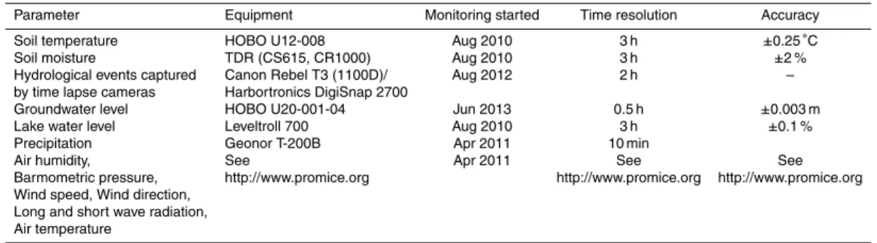
Table 1a.List of used equipment, start of monitoring and time resolution and accuracy for each

parameter for all monitoring data.

Parameter Equipment Monitoring started Time resolution Accuracy

Soil temperature HOBO U12-008 Aug 2010 3 h ±0.25◦

C

Soil moisture TDR (CS615, CR1000) Aug 2010 3 h ±2 %

Hydrological events captured Canon Rebel T3 (1100D)/ Aug 2012 2 h –

by time lapse cameras Harbortronics DigiSnap 2700

Groundwater level HOBO U20-001-04 Jun 2013 0.5 h ±0.003 m

Lake water level Leveltroll 700 Aug 2010 3 h ±0.1 %

Precipitation Geonor T-200B Apr 2011 10 min

Air humidity, See Apr 2011 See See

Barmometric pressure, http://www.promice.org http://www.promice.org http://www.promice.org Wind speed, Wind direction,

(29)

ESSDD

7, 713–756, 2014

catchment

E. Johansson et al.

Title Page

Tables Figures

◭ ◮

Back Close

Full Screen / Esc

Discussion

P

a

per

|

Discussion

P

a

per

|

Discussion

P

a

per

|

Discussion

P

a

per

|

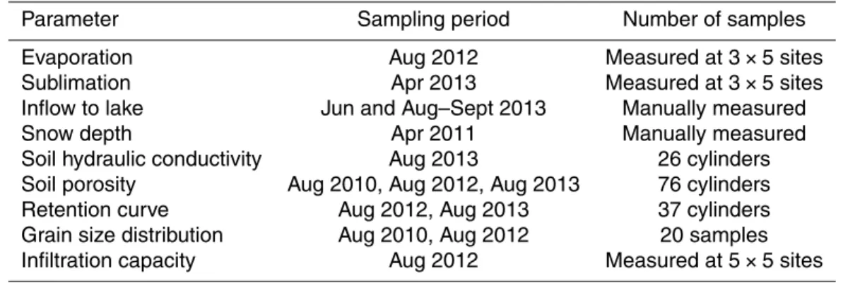
Table 1b.List of measured parameters and investigation period for non monitoring data.

Parameter Sampling period Number of samples

Evaporation Aug 2012 Measured at 3×5 sites

Sublimation Apr 2013 Measured at 3×5 sites

(30)

ESSDD

7, 713–756, 2014

catchment

E. Johansson et al.

Title Page

Tables Figures

◭ ◮

Back Close

Full Screen / Esc

Discussion

P

a

per

|

Discussion

P

a

per

|

Discussion

P

a

per

|

Discussion

P

a

per

|

Table 2.Levels of top of casing (TOC) and ground surface for each groundwater well relative

to the lake surface. Automatic monitoring in the well is marked by an X.

Well TOC Ground surface Automaic ID (m relative lake) (m relative lake) monitoring

1 5.45 4.96 X

2 8.85 8.23

3 12.35 11.6 X

4 9.07 8.39 X

5 12.19 11.8

6 4.79 4.16 X

7 10.7 10.07

8 20.69 20.09 X

9 4.73 3.98 X

11 13.56 12.91

12 21.99 21.51 X 13 0.2 −0.38 X

14 −4.79 −5.15 X