Annales
Geophysicae
An interpretation of the
fo
F2 and
hm
F2 long-term trends in the
framework of the geomagnetic control concept
A. V. Mikhailov1and D. Marin2
1Institute of Terrestrial Magnetism, Ionosphere and Radio Wave Propagation, Troitsk, Moscow Region 142190, Russia 2National Institute of Aerospace Technology, El Arenosillo, 21130 Mazagon-Moguer (Huelva), Spain
Received: 20 August 2000 – Revised: 19 February 2001 – Accepted: 22 March 2001
Abstract.Earlier revealed morphological features of thefoF2 andhmF2 long-term trends are interpreted in the scope of the geomagnetic control concept based on the contemporary F2-layer storm mechanisms. The F2-layer parameter trends strongly depend on the long-term varying geomagnetic ac-tivity whose effects cannot be removed from the trends using conventional indices of geomagnetic activity. Therefore, any interpretation of thefoF2 andhmF2 trends should consider the geomagnetic effects as an inalienable part of the trend analysis. Periods with negative and positivefoF2 andhmF2 trends correspond to the periods of increasing or decreasing geomagnetic activity with the turning points around 1955, and the end of 1960s and 1980s, wherefoF2 andhmF2 trends change their signs. Such variations can be explained by neu-tral composition, as well as temperature and thermospheric wind changes related to geomagnetic activity variations. In particular, for the period of increasing geomagnetic activity (1965–1991) positive at lower latitudes, but negative at mid-dle and high latitudes,foF2 trends may be explained by neu-tral composition and temperature changes, while soft elec-tron precipitation determines nighttime trends at sub-auroral and auroral latitudes. A pronounced dependence of thefoF2 trends on geomagnetic (invariant) latitude and the absence of any latitudinal dependence for thehmF2 trends are due to dif-ferent dependencies of NmF2 andhmF2 on main aeronomic parameters. All of the revealed latitudinal and diurnalfoF2 andhmF2 trend variations may be explained in the frame-work of contemporary F2-region storm mechanisms. The newly proposed geomagnetic storm concept used to explain F2-layer parameter long-term trends proceeds from a natural origin of the trends rather than an artificial one, related to the thermosphere cooling due to the greenhouse effect. Within this concept, instead of cooling, one should expect the ther-mosphere heating for the period of increasing geomagnetic activity (1965–1991).
Correspondence to:A. V. Mikhailov ([email protected])
Key words. Ionosphere (ionosphere-atmosphere interactions; ionospheric disturbances)
1 Introduction
ex-tract long-term trends from the ionospheric observations and the success of analysis depends, to a great extent, on the method employed. The useful “signal” is very small and the “background” is very noisy, so special methods are required to reveal a significant trend in the observedfoF2 andhmF2 variations. An approach being developed by Danilov and Mikhailov (1998, 1999), Mikhailov and Marin (2000) and Marin et al. (2001) has allowed us to find systematic vari-ations infoF2 andhmF2 trends unlike the other approaches (e.g. Bremer, 1998; Upadhyay and Mahajan, 1998), which result in a chaos of various signs and magnitudes of the trends at various stations. An application of this approach in foF2 trend analysis resulted in a geomagnetic control concept (Mikhailov and Marin, 2000) used to explain the revealed latitudinal and diurnal variations of thefoF2 trends. The ef-ficiency of this approach was also demonstrated by Marin et al. (2001) in the hmF2 trend analysis for many ionosonde stations in the Eurasian longitudinal sector. Briefly, the main results of the analysis by Mikhailov and Marin (2000) and Marin et al. (2001) are the following:
1. ThefoF2 trends demonstrate a pronounced dependence on geomagnetic (invariant) latitude with strong negative trends at high latitudes and small negative or positive trends at lower latitudes for the period of 1965–1991. Contrary to this, thehmF2 trends show no latitudinal dependence being positive at the majority of the stations analyzed. ThefoF2 and hmF2 trends are shown to be significant for most of the stations considered.
2. There are well pronounced (especially forfoF2) diurnal variations of the trend magnitude, while seasonal varia-tions are rather small and may be ignored compared to diurnal ones.
3. ThefoF2 trend analysis has shown that there exists peri-ods with negative and positivefoF2 trends, which corre-spond to the periods of long-term increasing/decreasing geomagnetic activity. In particular, the period of 1965– 1991 corresponds to the increasing geomagnetic activ-ity, while the geomagnetic activity was decreasing dur-ing the 1955–1965 period.
4. The geomagnetic control concept has been proposed to explain main morphological features of the foF2 and hmF2 trends revealed. This newly proposed geomag-netic hypothesis proceeds from a natural origin of the trends rather than an artificial one, related to the ther-mosphere cooling due to the greenhouse effect. The aim of the paper is to provide further analysis and phys-ical interpretation of the foF2 and hmF2 trends within the proposed geomagnetic control hypothesis.
2 Diurnal variations at different latitudes
The final version of the method used for the F2-layer param-eter trends analysis is given by Mikhailov and Marin (2000),
therefore, only a fragmentary description is presented here. All available observations at about 30 European, North Amer-ican and Asian ground-based ionosondes are used in the anal-ysis by Mikhailov and Marin (2000), and Marin et al. (2001) to revealfoF2 andhmF2 trends. The stations are located be-tween 38◦N and 81◦N geographic latitude (30◦N and 71◦N geomagnetic latitude) and cover a broad longitudinal range, which provides the possibility to study spatial variations of the trend magnitude. Trends are analyzed for relative devia-tions of the observedfoF2 orhmF2 values from some model δp = (pobs−pmod)/pmod wherep is the 12-month
run-ning mean of the monthly medianfoF2 orhmF2. A regres-sion (third-degree polynomial) ofpwith the sunspot number R12 is used as a model (Model 1). A regression ofpversus
R12 and annual meanAp12 index is refered to as Model 2.
Both models were used by Mikhailov and Marin (2000), and Marin et al. (2001) to find the slopeK (in 10−4per year) of linear trends for each station, for 12 months, and 24 LT moments. Although we are aware of the seasonal variations in trends (Danilov and Mikhailov, 1999), the later analysis has shown that diurnal variations may be much stronger than seasonal ones. Therefore, we analyze annual mean trends for selected LT hours. Averaged over 12 months theδpF2 value is found and this value is considered to be the annual mean value used in the trend analysis. The use of Model 2 was an attempt to exclude the effect of geomagnetic activity af-ter Bremer (1998) and Jarvis et al. (1998). But our analysis (Mikhailov and Marin, 2000; Marin et al., 2001) has shown that such an inclusion ofApindices to the regression, in fact, does not remove the geomagnetic effect, but only contami-nates the analyzed material. Therefore, Model 1 (regression withR12) is used in further analysis.
The magnitude of revealedfoF2 tends demonstrates strong diurnal variations depending on geomagnetic (invariant) lat-itude (Mikhailov and Marin, 2000). No systematic latitudi-nal variations were found for thehmF2 trends (Marin et al., 2001). Some examples of thefoF2 andhmF2 trend diurnal variations are given in Fig. 1 for auroral station Sodankyla (8inv=63.59◦), sub-auroral station Lycksele (8inv=61.46◦),
mid-latitude station Ekaterinburg (8inv=51.45◦), and lower
latitude station Alma-Ata (8inv = 35.74◦). These stations
are in the list analyzed by Mikhailov and Marin (2000), and Marin et al. (2001). Observations for the 1965–1991 period were used in further analysis. As in Mikhailov and Marin (2000) the(m+M)year selection was used for thefoF2 trend analysis, where(m)represents the years around solar minima and(M)represents the years around solar maxima; all years were used to analyzehmF2 trends (Marin et al., 2001).
bot-Fig. 1. Diurnal variation of annual mean slopeKforfoF2 (left panel) andhmF2 (right panel) trends at auroral, sub-auroral, mid-latitude and lower latitude stations for the 1965–1991 period, invariant latitudes are given in brackets. Error bars present the standard deviation of seasonal (over 12 months) scatter in the slopeK.
tom). Positive significant hmF2 trends for all LT are revealed at most of the stations considered (Marin et al., 2001), but at some stations, negative significant trends take place; therefore, an additional analysis is required to find out the reason. The Shimazaki (1955) formula which converts
Fig. 2. Same as Fig. 1, but for correlation coefficientsr(δfoF2,Ap12)andr(δhmF2,Ap12). Solid squares are correlation coefficients significant at the 95% confidence level, open squares – the coefficients which are insignificant at this level.
to the Shimazaki (1955) formula may not be useful for the hmF2 trend analysis, as this ratio itself demonstrates long-term variations. The other problem with usingfoE is in the absence of observations on many stations as well as during nighttime hours.
The revealedfoF2 and hmF2 trends may be explained in the framework of contemporary F2-layer storm mechanisms
corre-sponding diurnal variation of thefoF2 andhmF2 trend mag-nitudes (Fig. 1), although the correlation coefficients (Fig. 2) are small and insignificant (open squares) at the chosen 95% confidence level for some periods of the day. Usually, as Fig. 2 shows, large correlation coefficientsr(δfoF2,Ap12) are significant at the 95% confidence level and the correla-tion may be of both signs depending on the latitude of the station considered.
Let us consider the obtained latitudinal and diurnal varia-tions of thefoF2 andhmF2 trends (Figs. 1, 2) in the frame-work of the geomagnetic control concept.
2.1 Lower latitudes
PositivefoF2 andhmF2 trends are revealed both for day-and nighttime hours at the lower latitude station, Alma-Ata. An analysis of the F2-layer storm mechanisms for the lower lat-itude station Havana, with the same8inv =35◦(L =1.5)
as Alma-Ata, was made by Mikhailov et al. (1995). Accord-ing to AE-C and ESRO-4 satellite observations, geomagnetic disturbances result in an increase in the atomic oxygen abso-lute concentration, presumably due to the disturbed thermo-spheric circulation and downwelling at low latitudes, while theR = (O/N2)storm/(O/N2)quietratio remains practically
unchanged at the heights of the F2-region (Pr¨olss and von Zahn, 1977; Skoblin and Mikhailov, 1996; Mikhailov et al., 1997). Using the well-known expression by Rishbeth and Barron (1960)
NmF2∼=0.75qm/βm∝ [O]m/[N2]m (1)
where ion production rateqmand linear loss coefficientβm
are given at the F2-layer maximum, it was shown by Mik-hailov et al. (1995) that
NmF2∝ [O]
2/3 1
Tn5/6 [O]
1
[N2]1 2/3
(2) where all concentrations are given now at a fixed height h1. This expression shows that NmF2 will increase provided
that the absolute atomic oxygen concentration [O] increases, while [O]/[N2] ratio may remain unchanged at any fixed level
(the situation we have according to satellite observations at lower latitudes). Such [O]/[N2] height variations are also
confirmed by model calculations (F¨orster et al., 1999; Rish-beth and M¨uller-Wodarg, 1999). Thus, an [O] increase due to downwelling motion related to global storm circulation re-sulting from storm-induced equatorward thermospheric wind can really contribute to the positive NmF2 storm effect, while R(O/N2) ratio remains unchanged. This [O] increase
pro-vides a background NmF2 growth (see also Rishbeth, 1991; Field et al., 1998). Additional NmF2 increase is due to en-hanced equatortward thermospheric wind (upward plasma drift), resulting from the auroral heating.
An increase in neutral temperature and concentrations, as well as in vertical plasma drift (due to the enhanced equa-torward wind), usually taking place during disturbed peri-ods, leads to the hmF2 increase. This may be seen from
an approximate expression forhmF2 (Ivanov-Kholodny and Mikhailov, 1986)
hm∼= H 3
n
ln[O]1+lnβ1+ln(H2/0.54d)o+cW (3) whereH = kTn/mgis the scale height and [O] is the
con-centration of atomic oxygen,β is the linear loss coefficient at a fixed heighth1,W(in m/s) is the vertical plasma drift,c
is a coefficient close to unity,d =1.38·1019·(Tn/1000)0.5
is a coefficient in the expression for the ambipolar diffusion coefficientD=d/[O].
The above scenario takes place in the ‘nighttime’ (relative to storm onset) longitudinal sector. In the ‘daytime’ sector, F2-layer positive storm effects with the NmF2 andhmF2 in-crease are primarily the result from the vertical plasma drift increase without changes in neutral composition and tem-perature (Pr¨olls, 1995; Mikhailov et al., 1995). The main mechanism of suchW increase is the background (poleward during daytime) and the storm-induced (equatorward) wind interaction. Depending on the storm intensity, this interac-tion may result either in a decrease of the background merid-ional thermospheric wind or in its reversal. In both cases, we obtain an increase in NmF2 andhmF2. Therefore, one should expect positive NmF2 andhmF2 trends for the 1965– 1991 period of increasing geomagnetic activity. Our previous analysis confirms the existence of NmF2 andhmF2 positive trends for the majority of the day (Fig. 1, bottom).
Negative F2-layer storm effects are known to be strongest in the early morning LT sector (Wrenn et al., 1987; Pr¨olls, 1991,1993 and references therein) due to the perturbed neu-tral composition with the decreased O/N2ratio advected
to-wards middle and lower latitudes by the thermospheric cir-culation. This effect is especially pronounced at middle lat-itudes (see later), but takes place with strongly decreased magnitude at lower latitudes as well (see Fig. 1, around 07 LT). The area with increased [O] shifts further equatorward in this case.
Interesting results demonstrate the correlation coeffi-cients diurnal variations (Fig. 2, bottom) which support the above discussed scenario. Large and significant coefficients r(δfoF2, Ap12)are found for afternoon and evening hours
when foF2 trends are large at Alma-Ata (Fig. 1, bottom). This tells us that the revealed positive foF2 trends are re-lated to geomagnetic activity by the physical mechanism be-ing discussed. Large and significant correlation coefficients r(δhmF2, Ap12) are obtained for all LT moments (Fig. 2, right hand, bottom). This is due to both processes ([O] or/and W increase related to the increased geomagnetic activity) which contribute to the hmF2 increase, as it follows from Eq. (3).
The daytime sunlit F2-region is sensitive to the increase in [O] and W, resulting in the NmF2 increase. Therefore, the correlation coefficientsr(δfoF2,Ap12)are largest and
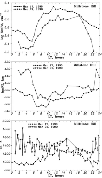
Fig. 3. Observed diurnal variations of NmF2,hmF2 and neutral temperatureTn estimated at Millstone Hill at 300 km for quiet 17
March 1990 and disturbed 21 March 1990 days.
nighttime correlation coefficients r(δfoF2, Ap12). In con-trast, the dependence ofhmF2 on [O] and W is practically the same during both daytime and nighttime hours. This gives large and significantr(δhmF2, Ap12)coefficients for
the whole day (Fig. 2, right hand, bottom). 2.2 Middle latitudes
Typical mid-latitudefoF2 andhmF2 trend diurnal variations are presented by the results at Ekaterinburg (Figs. 1,2). Neg-ative (especially at night) foF2 and positive hmF2 (all day long) trends are obtained for most of the mid-latitude stations considered (Mikhailov and Marin, 2000; Marin et al., 2001). For better illustration of the physical mechanisms involved, let us consider Millstone Hill incoherent scatter observations for quiet 17 March 1990 (Ap =3) and disturbed 21 March 1990 (Ap=76) days. Millstone Hill and Ekaterinburg have
close geomagnetic latitudes; therefore, such a comparison of the two stations is justified. Observed diurnal variations of NmF2,hmF2 andTn at 300 km are shown for the two days
in Fig. 3. The observations illustrate well-known and typ-ical negative storm behavior for the mid-latitude F2-layer. When we pass from quiet to disturbed conditions, NmF2 de-creases andhmF2 increases during both daytime and night-time hours. The NmF2 decrease is more pronounced in the nighttime and early morning LT sector. The same diurnal variation is seen in thefoF2 trends (Fig. 1, left panel), with the correlation coefficientsr(δfoF2,Ap12)being the largest
for the same hours (Fig. 2, left panel). Mid-latitude neg-ative F2-layer storm effects are known to be the strongest in the post-midnight-early-morning LT sector and they are much weaker in the afternoon (Wrenn et al., 1987; Pr¨olss, 1991,1993). As it was pointed out earlier, this is due to the disturbed neutral composition with a decreased O/N2ratio,
which is advected towards middle latitudes during the night, rotates into the day sector being shifted back to higher lati-tudes by diurnal varying thermospheric circulation (Skoblin and F¨orster, 1993; Fuller-Rowell et al., 1994; Pr¨olss, 1995). This effect is clearly seen in the afternoon with a tendency for thefoF2 trends to be even positive around 15 LT.
Contrary to the NmF2 behavior, hmF2 is larger for dis-turbed conditions. This is due to three reasons (see Eq. 3): 1) neutral temperatureTnis higher in the perturbed
thermo-sphere. Millstone HillTn estimations are shown in Fig. 3
(bottom); 2) linear loss coefficientβ =γ1[N2] +γ2[O2]is
higher for disturbed conditions due to higher molecular con-centrations and reaction rate coefficients depending on tem-perature; 3) vertical plasma drift W is more positive due to an enhanced equatorward thermospheric wind in the night-time sector, or to a decreased or even a reversal of the so-lar driven northward wind in the daytime LT sector (Pr¨olss, 1993; Wickwar, 1989).
Let us consider these changes in the thermospheric pa-rameters using Millstone Hill observations for 17 March and 21 March 1990. A self-consistent approach to the ionospheric F2-layer modelling proposed by Mikhailov and Schlegel(1997) with later modifications by Mikhailov and F¨orster (1999) and Mikhailov and Schlegel (2000) may be applied for daytime Millstone Hill observations to extract the set of main aeronomic parameters for the two days in ques-tion. The method uses measured Ne(h), Te(h), Ti(h), and
Vz(h)profiles to find the set of main aeronomic parameters
responsible for the observedNe(h)distribution in the
day-time F2-region. The calculated parameters are given in Ta-ble 1.
The results of the calculations are in agreement with the contemporary understanding of the F2-layer storm mecha-nisms (e.g. Rishbeth, 1991; Pr¨olss, 1995; Field et al., 1998). The calculations show an increase in exospheric temperature Tex(compare to Millstone Hill estimates at 300 km in Fig. 3),
a strong enrichment of the thermosphere with heavy molecu-lar species O2and N2, and an increase in W. The latter results
Table 1.Calculated thermospheric parameters for quiet 17 March 1990 and disturbed 21 March 1990 days at 300 km and 13.5 LT
Date Tex log [O] log [O2] log [N2] β/10−4 W
K cm−3 cm−3 cm−3 s−1 m s−1
17 Mar 90 1310 8.955 6.909 8.364 2.63 −8.1
21 Mar 90 1502 9.065 7.386 8.697 9.26 −3.8
Atomic oxygen concentration demonstrates a small increase at 300 km (around 25%), but in fact, this means a depletion of the [O] abundance in the thermosphere asTex(and
corre-sponding neutral scale height) is higher on 21 March (Table 1). A strong increase in [N2], [O2] as well as in the
tempera-ture results in aβincrease by more than a factor of 3 and this is the main reason for the NmF2 decrease on the disturbed day (see Eqs. 1,2). The growth ofβ,W, and [O] on the dis-turbed day results in higher observedhmF2 (Fig. 3, and Eq. 3).
Therefore, the analyzed period of 1965–1991 of increas-ing geomagnetic activity should result in negative NmF2 and positive hmF2 trends, as our previous analysis has shown (Mikhailov and Marin, 2000; Marin et al., 2001). Unlike the case with lower latitudes (Alma-Ata station) where changes in vertical plasma drift and atomic oxygen concentration are responsible for the positive F2-layer storm effects, neutral composition (O/N2ratio) and temperature changes are
sup-posed to be the main physical reason for the F2-layer nega-tive storm effects at mid-latitudes (Pr¨olss, 1995; Field et al., 1998), although the role of vibrationally excited N#2is consid-ered in some publications as well (e.g. Pavlov, 1994; Pavlov et al., 1999). The largest neutral composition (O/N2 ratio)
perturbations take place in the post-midnight-early-morning LT sector (Pr¨olss, 1980, 1993) and the calculated correla-tion coefficientsr(δfoF2,Ap12)are the largest for this part of the day (Fig. 2, left panel). Similar to the lower latitude case positivehmF2 trends and large correlation coefficients r(δhmF2,Ap12)take place practically all day long. As
men-tioned above, this is mainly due to the increase inβ,Tn and
W.
Therefore, the revealed mid-latitudefoF2 andhmF2 trends may be considered as the manifestation of the storm induced neutral composition, and temperature and meridional wind changes, which should take place for the period of increasing geomagnetic activity 1965–1991.
2.3 High latitudes
The situation is more complicated with the high-latitude F2-layer where close stations may demonstrate different diur-nal variations of the trend magnitude. As an example, So-dankyla (67.40 N; 26.60 E;8inv = 63.59 N) and Lycksele
(64.70 N; 18.80 E;8inv = 61.46 N) stations are shown in
Fig. 1. Very strong negativefoF2 trends take place during daytime with the minimum shifted to the morning hours at Sodankyla. The observedfoF2 trends are small with a pretty large scatter during morning and evening hours. The
correla-tion coefficientsr(δfoF2,Ap12)are large and significant
dur-ing daytime hours (Fig. 2, left-hand, top). On the contrary, at Lycksele, the largest negativefoF2 trends are observed in the evening LT sector, while the trends are small during the first part of the day. Corresponding diurnal variation is seen forr(δfoF2,Ap12)in Fig, 2 where large and significant cor-relation coefficients are found for the second part of the day. The Sodankyla station also shows an interesting and un-usualhmF2 trend diurnal variations (Fig. 1, right-hand, top), when compared to other stations. The trends are positive although small during daytime hours, but they are negative at nighttime. The daytime correlation coefficientr(δhmF2, Ap12)are large and significant, while the nighttime values are small and insignificant at the 95% confidence level (Fig. 2, right-hand, top). Such unusual diurnal variations of the hmF2 trend magnitude are discussed later using EISCAT ob-servations. Large positivehmF2 trends along with large and significant correlation coefficientsr(δhmF2,Ap12)take place
during the whole day at Lycksele (Figs. 1, 2; right-hand pan-els).
Let us start with thefoF2 trends (Fig. 1, left-hand, top). The Sodankyla station (8inv = 63.59◦) is located in the
plasma ring or FLIZ zone (Thomas and Andrews, 1969; Pike, 1971) where an intensive F2-region ionization is produced by soft electron precipitation (Morse et al., 1971). The equato-rial boundary of this zone is located at8inv = 61−62◦ at
00–06 MLT and at8inv = 63◦ at 18–21 MLT while
dur-ing daytime, it shifts northward at8inv=70−72◦(Sagalin
and Smiddy, 1974). This excursion of the precipitation zone explains the appearance of two peaks in thefoF2 trend di-urnal variation (Fig. 1, left-hand, top). As the intensity of electron precipitation is highly variable in the FLIZ zone, the scatter of the trends obtained is fairly large and the correla-tion coefficients r(δfoF2,Ap12)are small and insignificant (Fig. 2, left-hand, top) for these two periods of the day. The corpuscular ionization should be strong enough during these periods to compensate large negative effect in NmF2 due to large changes in neutral composition and temperature expected in the perturbed auroral thermosphere. The latter is seen for daytime hours when, despite direct solar photoion-ization, very strong negativefoF2 trends are observed (Fig. 1. left-hand, top).
The sub-auroral station Lycksele (8inv = 61.46◦) turns
out to be in the FLIZ zone in the morning but not in the evening and unlike Sodankyla, there is only one (morning) peak wherefoF2 trends are small and correlation coefficients r(δfoF2,Ap12)are small and insignificant (Fig. 2, left second
Fig. 4. Observed with EISCAT diurnal variations of NmF2,hmF2 and electric fields for quiet 17 November 1987 and disturbed 19 November 1987 days.
shifts to the latitudes8inv=70−72◦(Sagalin and Smiddy, 1974) and we have strong negativefoF2 tends resulting from the disturbed neutral composition and temperature similar to the middle latitude case. It should be kept in mind that neu-tral composition and temperature are perturbed for the whole day and this explains the large positive and significanthmF2 trends at Lycksele for all LT moments (Figs. 1,2, right sec-ond panels).
Let us analyzehmF2 trends at Sodankyla, where positive daytime trends and negative (although insignificant at the 95% confidence level) nighttimehmF2 trends are obtained (Figs. 1,2, right-hand, top). Such variations are due to spe-cific mechanisms of the auroral F2-region formation.
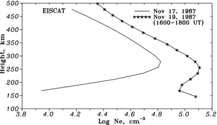
Observed with EISCAT NmF2,hmF2 and electric fieldE diurnal variations are shown in Fig. 4 for quiet 17 Novem-ber 1987 (Ap =3) and moderately disturbed 19 November (Ap=12) days. Electric fieldsE ≈20−40 mV/m and an
Fig. 5. Observed with EISCAT medianNe(h)profiles calculated
over two hours. Note the effect of strong particle precipitation in theNe(h)height distribution on 19 November.
intensive electron precipitation took place on 19 November, while both characteristics were small on 17 November (some splashes of electric field took place only after 19 UT). Ob-served NmF2 are higher andhmF2 are lower on 19 Novem-ber for the period of 16–22 UT, when an intensive electron precipitation is expected (Fig. 1, left-hand, top). Large scat-ter in the observedhmF2 is seen on 19 November and is obvi-ously due to a varying precipitation intensity. MedianNe(h)
profiles found over the 16–18 UT period are given in Fig. 5 for the two days in question. Strong precipitation results in an enhanced electron concentration (especially in the lower F-region) as well as in a decrease inhmF2. Namely, this ef-fect of the electron precipitation is the most important for our analysis. Strong plasma production at lower altitudes shifts normal hmF2 to lower heights (e.g. Torr and Torr, 1969). A similar situation exists for a normal mid-latitude F2-layer when daytimehmF2 is lower than nighttimehmF2dian over one hour for one and the same input parameters. This is due to strong solar photoionization at low F-region heights. As the precipitation intensity increases with geomagnetic activ-ity (Sato and Colin, 1969; Marubashi, 1970), nighttimehmF2 trends are negative at Sodankyla (Fig. 1, right-hand, top) for the period of increasing geomagnetic activity of 1965– 1991. Therefore, the revealed features of the NmF2 and hmF2 nighttime trends may be attributed to the electron pre-cipitation effects.
Besides particle precipitation strong electric fields are an inalienable feature of the disturbed auroral F2-region. The observed increase in geomagnetic activity for the analyzed period of 1965–1991 is the manifestation of intensified elec-tric fields in the auroral zone. Joule heating related to the electric fields results in strong perturbations of neutral com-position (O/N2, O/O2decrease) and neutral temperature
in-crease (e.g. Pr¨olss, 1980; Rishbeth and M¨uller-Wodarg,-1999). Therefore, by analogy with the mid-latitude case, one should expect strong negative foF2 and positivehmF2 trends for the period in question. An additional effect work-ing in the same direction is due to the dependence of the O++N
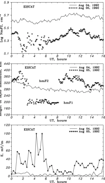
Fig. 6. Observed with EISCAT diurnal variations of NmF2,hmF2 and electric fields for quiet 04 August 1992 and disturbed 05 August 1992 days. Note the decrease in the height of the layer maximum after a strong electric field is switched on.
on electric field E (Schunk et al, 1975). Strong negativefoF2 trends (Fig. 1, left-hand, top) do take place at Sodankyla dur-ing daytime hours, the nighttime case was discussed above. But relatively small (although positive) daytimehmF2 trends (Fig. 1, right-hand, top) look rather strange. At least three reasons may be considered:
1) the accuracy of initial experimentalM(3000)F2 values, and theM(3000)F2 tohmF2 conversion procedure used; 2) the effect of strong electric fields on theNe(h)height
pro-file;
3) the effect of the auroral thermosphere depletion (due to upwelling) with atomic oxygen (Pr¨olss, 1980).
Let us consider EISCAT observations for quiet 04 August 1992 (Ap=2) and disturbed 05 August 1992 (Ap=35) days which may help us analyze the problem with thehmF2 day-time trends. The daily meanApindex was 15 on 04 August
Fig. 7.Observed with EISCATNe(h)profiles for different UT
mo-ments of the disturbed day 05 August 1992. Note the modification of normal F2-layer and formation of the layer maximum around 200 km as a reaction to the strong increase in the linear loss coefficient β. Quiet timeNe(h)profiles for 04 August 1992 are shown for a
comparison.
due to a disturbance which started late in the afternoon. Yet the first half of the day considered here was very quiet and we acceptedAp = 2 for our model calculations. Observed NmF2,hmF2, as well as electric field diurnal variations, are shown for the two days in Fig. 6.
The selected couple of dates demonstrates the effect of the general NmF2 decrease for the disturbed day which corre-sponds to thefoF2 negative trend (Fig. 1, left-hand, top) for the considered period of increasing geomagnetic activity of 1965–1991. The effect of the electric field switching on and off is also seen in Fig. 6. The medianNe(h)profiles taken
over a set of one hour observations are shown in Fig. 7 for some UT periods. Two quiet time (04 August 1992)Ne(h)
profiles are shown for a comparison as well. An abrupt de-crease of the layer height down to 200 km (F1-layer) takes place during the morning hours on 05 August (Fig. 6, mid-dle panel) as a reaction to the enhanced electric field (Fig. 6, bottom). Later in the morning, whenEdecreases and the photoionization rate increases, hm restores back to normal hmF2 values around 350 km. In the afternoon, a moderate Eincrease again results in thehmF2 decrease, whenhmF2 turns out to be close to the 04 August values.
All observed disturbed Ne(h) profiles (Fig. 7) show a
strongly reduced NmF2 up to a complete disappearance of the F2-layer (0300–0800 UT period), while a pronounced F1-layer appears around 200 km height. It is obvious that theM(3000)F2 parameter, determined from routine ground-based ionosonde observations, is not reliable for such pro-files. On the other hand, special care is required when tak-ing into account the effect of the underlytak-ing ionization in the empirical formulas relatingM(3000)F2 tohmF2. Therefore, hmF2 derived fromM(3000)F2 may not be very reliable for such Ne(h) profiles, but one may hope that this does not
Table 2.Calculated at 300 km thermospheric parameters for quiet 04 August 1992 and disturbed 05 August 1992 days and two periods of the day
Date Tex log [O] log [O2] log [N2] β/10−4 W
K cm−3 cm−3 cm−3 s−1 m s−1 04 Aug 92, 06–07 UT 1088 8.546 6.807 8.241 1.84 +4.3 05 Aug 92, 06–07 UT 1332 8.345 7.422 8.593 15.6 +28.5 04 Aug 92, 11–12 UT 1158 8.645 6.793 8.279 1.96 −16.8 05 Aug 92, 11–12 UT 1263 8.537 7.235 8.512 8.77 +31.3
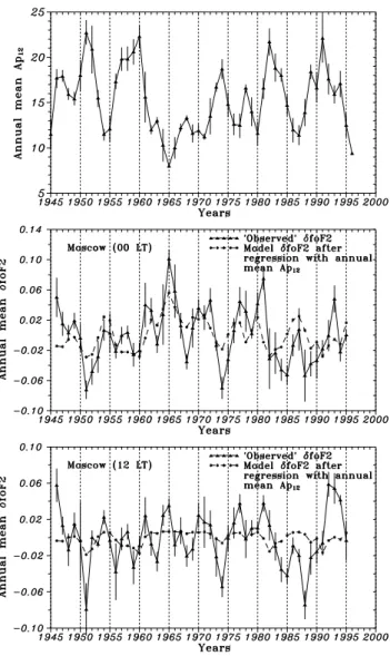
Fig. 8.Annual mean and 11-year running meanApindex variations. Symbols(m)and(M)refer to years of solar cycle minimum and maximum.
To illustrate the changes in the thermospheric parameters responsible for the observed NmF2 andhmF2 variations un-der disturbed conditions, let us consiun-der two sunlit periods around 0630 and 1130 UT for 04 and 05 August. The above mentioned method by Mikhailov and Schlegel (1997) with later modifications is used for this analysis. The two cho-sen UT periods correspond to the cases of a pronounced F1-layer appearance (0600–0700 UT) and to a moderately dis-turbed F2-layer with a pronouncedhmF2 (1100–1200 UT); the correspondingNe(h)profiles are shown in Fig. 7.
Cal-culated thermospheric parameters for the quiet and disturbed days are given in Table 2. The calculatedTex is higher on
05 August (the disturbed day), especially for the morning period when strong electric fields were observed. The en-hanced electric field produces an intensive Joule heating and an upwelling in the thermosphere. The latter is seen in the calculated vertical plasma driftW (Table 2). The upwelling motion results in a [O] decrease and a [O2], [N2] increase,
which is also seen for the disturbed day with respect to the quiet one. Relatively small [O] decrease at 300 km (58% in the morning and 28% at around noon), in fact, corresponds to a strong decrease in the atomic oxygen abundance, asTex
(and corresponding neutral scale height) is higher on 05 Au-gust (Table 2).
The thermosphere heating and upwelling results in the str-ong increase in [N2] (by a factor of 2.25 in the morning and
by 1.71 times around noon), and in the [O2] increase by a
factor of 4.12 and 2.77, respectively. This [N2] and [O2]
increase, along with the increase in the O++N
2rate constant
depending onTn,TiandE, results in a very strongβincrease
by a factor of 8.5 in the morning case, and by a factor of 4.5 around noon. Similar to the mid-latitude case, this increase in the linear loss coefficientβis the main reason for the NmF2 decrease on the disturbed day; the additional negative effect in NmF2 is related to the [O] decrease. This analysis based on EISCAT observations illustrates the physical mechanism of the strongfoF2 negative trend obtained for daytime hours at Sodankyla (Fig. 1, left top panel).
Electric fields via the chain of the processes mentioned above strongly affect theNe(h)height distribution andhmF2,
accordingly. During nighttime, when direct solar photoion-ization is absent, or in the morning, when it is not strong enough, the loss coefficientβ increase may result in a com-plete disappearance of the normal F2-layer and formation of theNe(h)profile with maximum around 200 km (Fig. 5, 03–
08 UT period). Such a layer is composed of heavy molecular ions, NO+and O+2, as model calculations show.
Therefore, electric fields along with the earlier discussed electron precipitation effect may really contribute to the neg-ative nighttimehmF2 trends at Sodankyla (Fig. 1, top right panel). During daytime hours, solar EUV ionization becomes strong enough and the F2-layer maximum is formed at usual heights, but a well-developed F1 layer still exists (Fig. 7), with the NmF2 and NmF1 values being close around 08 UT (Figs. 6,7).
Both satellite observations (Pr¨olss, 1980) and model cal-culations (Table 2) show a decrease in the atomic oxygen concentration for disturbed conditions. According to Eq. (3), a decrease in [O] should compensate to some extent for the hmF2 growth, primarily resulting from theβ,W andTn
in-crease on the disturbed day. This effect is not strong for the 04 and 05 August case (1lg[O]=−0.108 and1lgβ=0.65) and disturbed daytimehmF2 values are larger than the quiet time ones (Fig. 6, middle panel). But, depending on the per-turbation intensity, the effect may be larger. For instance, an analysis of EISCAT observations for the period of geomag-netic storm on 10 April 1990 (Mikhailov and Schlegel, 1998) has revealed an [O] decrease by a factor of 4.3 at 300 km, with respect to the previous day. In that case, the daytime layer maximum was formed around 200 km height.
stations) daytimehmF2 trends at Sodankyla (Fig. 1, right top panel) may be due to a strong decrease in the atomic oxygen abundance in the perturbed auroral thermosphere.
3 Discussion
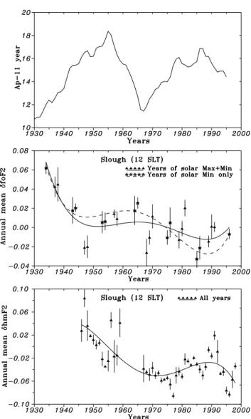
Investigation of the ionospheric trends was greatly stimulated by the model calculations of Rishbeth (1990), and Rishbeth and Roble (1992), which predicted the ionospheric effects of the atmosphere greenhouse gas concentration increase. Since then, researchers have been trying to reveal the predicted thermosphere cooling analyzing ionospheric trends (Bremer, 1992; Givishvili and Leshchenko, 1994; Ulich and Turunen, 1997, Jarvis et al., 1998; Upadhyay and Mahajan, 1998). But the world-wide pattern of the F2-layer parameter trends turned out to be very complicated and cannot be reconciled with the greenhouse hypothesis. On the contrary, the geo-magnetic control concept by Mikhailov and Marin (2000), based on the contemporary understanding of the F2-layer storm mechanisms, allows us to explain the revealed mor-phological features of the F2-layer trends. According to this concept, there are periods of negative and positive F2-layer parameter trends corresponding to the long-term changes in geomagnetic activity shown in Fig. 8. Annual meanAp in-dices prior 1932 were reconstructed fromaaindices avail-able from 1868. Years of solar cycle minima(m)and max-ima (M) are marked in Fig. 8 as well, to show that such long-term variations in geomagnetic activity (presented by 11-yearApindex) are not related to solar cycle variations. A steady increase in geomagnetic activity took place for the period from 1900 to middle of 1950s followed by a decrease towards middle of 1960s and again an increase towards the end of 1980s. A tendency for a decrease in geomagnetic ac-tivity after 1990 is clearly seen in annual meanApvalues. Similar variations of geomagnetic activity can be found in Clilverd et al., (1998, their Fig. 6). Namely, these long-term variations in geomagnetic activity result in the ionospheric F2-layer long-term trends.
An example of such long-term variations is given in Fig. 9 for a mid-latitude station Slough, where ionospheric ob-servations are available from the early 1930s. Variations of the 11-yearApindex are repeated in Fig. 9 (top) for further discussion. TheδfoF2 variations are considered for (M+ m)and(m)year selections (Danilov and Mikhailov, 1999; Mikhailov and Marin, 2000). Solid and dashed lines are the least squares fitting by the 4th degree polynomial (a higher degree gives practically the same results). Everywhere er-ror bars present the standard deviation over 12 monthly val-ues. An anti-phase type ofδfoF2 andAplong-term variations is seen for the period in question. The periods of increas-ing geomagnetic activity (before 1955 and after the end of the 1960s) are seen to correspond to negativefoF2 trends, while during the decreasing phase of geomagnetic activity (1955 to the end of the 1960s), a small positivefoF2 trend takes place. There is also a tendency for thefoF2 trend to switch from negative to positive after 1990, in accordance
Fig. 9.11-year running meanApindex along withδfoF2 andδhmF2 long-term variations. Two year selections (M +m) and (m)(see text) are used for thefoF2 and (all years) for thehmF2 trend analy-sis. Least squares fitting curves are a 4th degree polynomials. Error bars present the standard deviation of seasonal (over 12 months) scatter.
with the change in geomagnetic activity (see Fig. 8). Dif-ferent signs of thefoF2 trends for the periods before and af-ter 1965 were demonstrated earlier by Mikhailov and Marin (2000) for some stations with long observational periods.
Fig. 10. Annual meanAp12 andδfoF2 variations at Moscow, 00 and 12 LT. Dashed line is an attempt to remove the dependence on geomagnetic activity usingδfoF2 regression withAp12. Note that observedδfoF2 variations are much stronger than model ones especially for daytime.
with geomagnetic activity variations are discussed earlier in the paper.
In the framework of the proposed geomagnetic hypothe-sis one should expect thermosphere heating rather than the cooling that the researchers are seaking when considering the 1970–1990 period. Indeed, from theApvariations (Fig. 8), one may accept theApindex increase from 12 to 16 for the period in question; such an increase in theApindex, ac-cording to the thermospheric MSIS-83 (Hedin, 1983) model, results in the annual meanTex increase by about 10 K for
mid-latitudes (F10.7 = 140 was used in calculations). But
this heating will be followed by the thermosphere cooling, in accordance with the long-term changes in the geomagnetic activity (Fig. 8).
Although there is an obvious relationship between the F2-layer parameter trends and the geomagnetic activity, it is
im-possible to remove this geomagnetic effect from the trends revealed, using any conventional index (e.g. monthly or an-nual meanAp) of geomagnetic activity, and to check if there is any residual trend (of a greenhouse origin, for instance). If it could be accomplished by using the conventional indices, the problem of the F2-layer storm description and prediction would have been solved long ago, but this has not been the case until now. This is not surprising as any global geomag-netic activity index cannot, in principle, take into account the whole complexity of F2-layer storm effects with positive and negative phases depending on the season, longitude, UT and LT of storm onset, storm magnitude, etc. Therefore, an inclusion of theApindex to the regression, in fact, does not remove the dependence on geomagnetic activity, as supposed by Bremer(1998) and Jarvis et al. (1998), but only contam-inates the analyzed data (Mikhailov and Marin, 2000). In-deed, according to Mikhailov and Marin (2000), and Marin et al. (2001), such an inclusion of theApindex has some effect on the trend magnitude, but without changing, in prin-ciple, the main morphological features of thefoF2 andhmF2 trends. A similar result was obtained by Ulich and Turunen (1997) who did not include theApindex in their study for this reason.
Figure 10 illustrates an attempt to remove the geomag-netic effect by the inclusion of the annual mean Ap12
to the foF2 trend analysis for Moscow, 00 and 12 LT. A two-step procedure was applied. At first, δfoF2 = (foF2obs−foF2mod)/foF2mod values were found and called
‘observed’ (Fig. 10, solid line). Then a regression (2nd de-gree polynomial) of theseδfoF2obs with annual meanAp12 was calculated and called ‘model’ in Fig. 10 (dashed line). The model curve is seen to follow, qualitatively, the ob-servedδfoF2 variation for 00 LT with a correlation coefficient r =0.538, which is significant at the 99% confidence level. But the observed δfoF2 variations are much larger and not reproduced completely by the model. The situation is even worse for daytime (12 LT) conditions. In this case, there is not even a qualitative agreement between the two curves (r=0.227, insignificant). The same result was obtained for Ekaterinburg (Fig. 2, left panel) where significant correlation coefficients were found only for nighttime hours.
The obtained result tells us that, in fact, the geomagnetic effect is much stronger (at least during nighttime) than can be described using theAp12 index. Poor δfoF2 correlation with Ap12 during the daytime confirms the complexity of the F2-layer storm mechanisms as mentioned earlier. For instance, mid-latitude daytime F2-layer storm effects may be due to thermospheric perturbations formed in the night-time longitudinal sector during the preceding geomagnetic storm (Skoblin and F¨orster, 1993; Fuller-Rowell et al., 1994; Pr¨olss, 1995).
On the other hand, one should keep in mind that the sunspot numberR12, usually used in empirical ionospheric models,
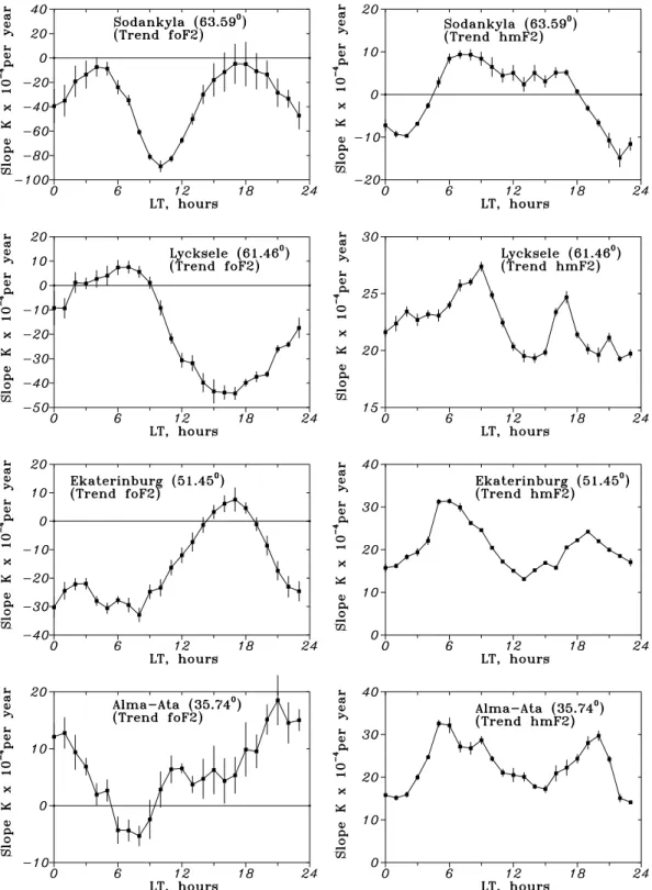
ex-Table 3.Annual mean slopeK(in 10−4per year) for the period after 1965 for the stations with close8inv, but differentD. Years of solar minimum(m)forfoF2 and all years forhmF2 trend analysis are used.
Station 8inv D sinIcosIsinD K(foF2) K(foF2) K(hmF2) K(hmF2)
deg deg 12 LT 06 LT 12 LT 06 LT
(m)years (m)years all years all years
Yakutsk 55.1 −15 −0.06 −43.4 −49.2 +15.9 +22.7
St.Petersburg 55.9 +7 +0.03 −27.3 −14.1 +10.1 +17.9
Slough 49.8 −7 −0.04 −25.3 −19.6 +17.2 +27.6
Tomsk 50.6 +9 +0.04 −20.2 −25.9 +23.2 +22.5
Khabarovsk 40.2 −11 −0.08 −5.0 −6.0 +13.5 +22.9
Novokazalinsk 39.5 +7 +0.05 −17.4 −38.0 −1.0 +15.1
tract F2-layer parameter trends the imperfection ofAp12and
R12indices results in a fairly largeδfoF2 andδhmF2 scatter
(e.g. Fig.10). In practice, it was recommended (Danilov and Mikhailov, 1999; Mikhailov and Marin, 2000) to use only the years around solar minima(m)or the years around solar maximum and minimum(M+m)for thefoF2 trend analy-sis. Such a selection of years allows us to avoid the hystere-sis effect which takes place at the falling and rising phases of the solar cycles, and when thefoF2 versusR12correlation is the worst. With this approach, it was possible to obtain the most consistent pattern of thefoF2 trends over all the sta-tions considered. On the contrary, the same approach turned out to be inefficient when applied to thehmF2 trend analysis and all available years were used in the study by Marin et al. (2001). This is rather strange as the hysteresis effect takes place forM(3000)F2 solar cycle variations as well (Rao and Rao, 1969). There is currently no explanation for this effect. A well-pronounced dependence of thefoF2 trend magni-tude on the geomagnetic (invariant) latimagni-tude (Danilov and Mikhailov, 1999; Mikhailov and Marin, 2000) is explained by the perturbed neutral composition and temperature latitu-dinal dependence, as discussed earlier in the paper. Contrary to this, no systematic latitudinal dependence was revealed for thehmF2 trends (Marin et al., 2001). This result may be ex-plained by thehmF2 dependence on the main aeronomic pa-rameters (Eq. 3). Normally, neutral concentrations (O, O2,
N2at a fixed level), temperatureTnas well as vertical plasma
driftWincrease during disturbed periods. According to Eq. (3), this should result in anhmF2 increase, as all terms in Eq. (3) work in one direction. Therefore, we have positive hmF2 trends at middle and lower latitudes; the high-latitude case was discussed earlier. The meridional windVnx effect
(viaW = VnxsinIcosIcosD) becomes efficient at lower
latitudes as magnetic inclinationI approaches 45◦. As the perturbation inβ andTn decreases and the [O] (see above)
andWcontributions increase towards lower latitudes, no pro-nounced latitudinal dependence for thehmF2 trend magni-tude should take place, in accordance with results of our study.
In principle, some longitudinal effect in thefoF2 andhmF2 trends may be expected in the scope of the proposed geo-magnetic control hypothesis. A statistical analysis by
Ha-jkowicz (1998) of AE-index variations over two solar cycles (1957–1968 and 1978–1986) has shown that the maximum in auroral activity is largely confined to 09–18 UT, with a dis-tinct minimum at 03–06 UT. This means that Eastern Siberia and Japan are primarily at night during the period of maxi-mum auroral activity, whereas Europe and Eastern America are primarily at daytime. This effect, overlapping with the background solar driven thermospheric circulation (equator-ward at night and pole(equator-ward during daytime), may give some longitudinal effects in the F2-layer parameter trends. An-other source of longitudinal variation is related to the zonal winds and longitudinally dependent magnetic declinationD via the wind term in the vertical plasma driftW. Primarily negativefoF2 and hmF2 trends at longitude west of 30◦E, yet positive trends east of 30◦E, were revealed by Bremer (1998). A tendency for similar hmF2 trend separation was reported by Marin et al. (2001). Indeed, the D = 0 line crosses Europe along the longitudeλ≈20◦E and the zonal wind effect cannot be excluded. But a preliminary analy-sis has shown that the situation is not that straightforward. Three pairs of stations with close 8inv, but different
mag-netic declinationD, are compared in Table 3, wherefoF2 and hmF2 trends from Mikhailov and Marin (2000) and Marin et al. (2001) are given for 12 and 06 LT. The results in Table 3 show that regardless of different signs of magnetic dec-lination D, foF2 trends are negative and hmF2 trends are positive at all stations considered (the daytimehmF2 trend at Novokazalinsk is insignificant), in accordance with the earlier obtained conclusions (Danilov and Mikhailov, 1999; Mikhailov and Marin, 2000; Marin et al., 2001). The ex-pected longitudinal effect may be due to vertical plasma drift W = (VnxcosD −VnysinI )sinIcosI variations, where
Vnx andVny are meridional and zonal components of the
thermospheric wind. Westward (Vny < 0) zonal wind is
strong around 06 LT, but small around 12 LT (Hedin et al., 1991). On the contrary, Vnx is small around 06 LT,
there-fore theVny effect may be expected around 06 LT. Table 3
small when compared to the contribution of other aeronomic parameters.
Some European stations were shown to demonstrate nega-tivehmF2 trends (Marin et al., 2001) and this was the reason to mention a longitudinal effect in thehmF2 trends. Their Ta-ble 2 (Model 1) shows that significant negative trends were revealed for some LT moments at Bekescsaba (46.7 N, 21.2 E), Poitiers (46.6 N, 0.3 E), Dourbes (50.1 N, 4.6 E) and Juliusruh (54.6 N, 13.4 E); the other stations may be consid-ered as sub-auroral and auroral ones, with specific mecha-nisms of the F2-layer formation discussed earlier in this pa-per. Therefore, an additional analysis is needed for these mid-latitude stations to find out the reason for suchhmF2 behavior. NegativehmF2 trends were reported for Southern hemisphere stations in the Argentine Islands and Port Stan-ley by Jarvis et al. (1998), and for Sodankyla by Ulich and Turunen (1997). The latter result should be discussed as it contradicts our conclusions obtained for the Sodankyla sta-tion.
It was stressed by Danilov and Mikhailov(1999), and Mik-hailov and Marin (2000) that F2-layer trend results are str-ongly dependent on the method used to extract the trends from the ionosonde observations. Ulich and Turunen (1997) obtained a negativehmF2 trend,−0.39 km/year for daytime hours over the period of 1958–1994. Unlike our approach, they worked with non-smoothed absolute deviations1hmF2 from a model (linear regressionhmF2 with monthly averaged F10.7), although they applied to1hmF2 a running mean
fil-ter with a width of 11 years in order to suppress solar activity effects. We have used a similar approach and did obtain neg-ative daytimehmF2 trends over the period in question. Re-garding this,the following should be mentioned:
1) non-smoothedhmF2 (orfoF2) values show a very large scatter where a “useful signal” may just be lost. Therefore, smoothing of the initial data and working with relative (not absolute) deviations from a model was recommended for the trend analysis (Danilov and Mikhailov, 1999; Mikhailov and Marin, 2000);
2) it is known that monthly medianfoF2 andM(3000)F2 pa-rameters correlate better with smoothed (not monthly aver-aged) indices of solar activity (e.g. Mikhailov and Mikhailov, 1999 and references therein). That is why only 12-month running mean sunspot numbersRorF10.7are used in
empir-ical F2-layer parameter modelling. Moreover, a non-linear dependence of F2-layer parameters on solar activity level provides better regression accuracy (e.g. Kouris et al., 1997) than the linear one used by Ulich and Turunen (1997); 3) as thehmF2 trend follows the geomagnetic activity, a sep-arate analysis is required for different periods in the geomag-netic activity’s long-term variations; the end of the 1960s and the beginning of the 1990s are the turning points in these variations. Therefore, a trend derived over the whole 1958– 1994 period does not correctly present the realhmF2 long-term variations.
Due to these differences in approaches, the daytimehmF2 trends at Sodankyla obtained by Ulich and Turunen (1997) and Marin et al. (2001) have a different sign for the period of
1965–1991.
4 Conclusions
The foF2 and hmF2 trend morphology earlier revealed by Danilov and Mikhailov (1999), Mikhailov and Marin (2000), and Marin et al. (2001), was interpreted in the framework of the geomagnetic control concept proposed by Mikhailov and Marin (2000). Latitudinal and diurnal variations of the an-nual mean foF2 andhmF2 trends are the most pronounced features and their analysis was the major concern of the pa-per. The main results may be listed as follows:
1. The effect of long-term varying geomagnetic activity is very strong in thefoF2 and hmF2 trends. But it is impossible to remove this geomagnetic effect from the F2-layer parameter trends using conventional (monthly or annual meanAp, for instance) indices of geomag-netic activity. An inclusion of Ap12 to the regression
removes only partly the geomagnetic effect, but con-taminates the analyzed material, in principle, without changing the obtained result. Therefore, any interpre-tation of thefoF2 andhmF2 trends should consider the geomagnetic effect as an inalienable part of the trends revealed, and this can be done based on the contempo-rary understanding of the F2-layer storm mechanisms. 2. Large and significant correlation coefficients r(δfoF2,
Ap12)andr(δhmF2,Ap12), as well as similarity in trends
and correlation coefficients diurnal variations (Figs. 1, 2) reveals the close relationship of the F2-layer parame-ter trends with geomagnetic activity. Both diurnal vari-ation patterns (Figs.1, 2) clearly indicate physical pro-cesses which are usually used to explain latitudinal and diurnal layer parameter storm variations. This F2-layer storm mechanism is based on the background so-lar driven and disturbed thermosphere circulation inter-action, resulting in neutral composition and temperature perturbations.
3. There are periods with negative and positivefoF2, and hmF2 trends which correspond to the periods of increas-ing or decreasincreas-ing geomagnetic activity. An 11-yearAp index can be used as an indicator of such long-term vari-ations in geomagnetic activity. The turning points are: around 1955, the end of the 1960s and the 1980s, where foF2 andhmF2 trends change their signs. An anti-phase for δfoF2 and syn-phase forδhmF2 type of long-term variations withApmay be followed for Slough, where ionospheric observations are available from the early 1930s. Such a type of mid-latitude F2-layer parame-ter variations is due to neutral composition, temperature and thermospheric winds changes related to geomag-netic activity variations.
are due to different dependencies of NmF2 andhmF2 on main aeronomic parameters, the latter being latitudinal dependent during disturbed periods. In particular, for the period of increasing geomagnetic activity of 1965– 1991, it may be concluded:
(a) at lower latitudes, positive (or small negative)foF2 trends and positivehmF2 trends are primarily due to an increase in the equatorward thermospheric wind and in atomic oxygen concentration;
(b) at middle latitudes, the negativefoF2 trend is due to neutral composition (O/N2 ratio decrease) and
temperature increase, resulting in the linear loss co-efficientβ = γ1[N2] +γ2[O2] increase. The
lat-ter, along with the enhancedTn and equatorward
thermospheric wind, determine the positivehmF2 trend;
(c) at sub-auroral and auroral latitudes,foF2 andhmF2 trends are determined by strong neutral composi-tion and temperature changes during daytime hours, while at nighttime, soft electron precipitation pro-vides strong contribution. In the auroral zone, elec-tric fields in addition to perturbing neutral composi-tion and temperature via Joule heating, can strongly affect the linear loss coefficientβ=γ1[N2]+γ2[O2]
via theγ1 dependence onE. This results in very
strong, negativefoF2 and relatively small, positive hmF2 daytime trends.
5. All the revealed morphological features of thefoF2 and hmF2 trends may be explained in the framework of con-temporary F2-region storm mechanisms. This newly proposed geomagnetic storm concept used to explain the F2-layer parameter long-term trends proceeds from a natural origin of the trends rather than an artificial one related to the thermosphere cooling due to the green-house effect. Within this concept, instead of the ther-mosphere cooling that the researchers are seeking, one should expect the thermosphere heating for the period of increasing geomagnetic activity of 1965–1991. This period will be followed by the thermosphere cooling, in accordance with the long-term changes in geomagnetic activity.
Acknowledgements. The authors thank the Director and the staff of EISCAT for running the radar and providing the data. The EISCAT Scientific Association is funded by scientific agencies of Finland (SA), France (CNRC), Germany (MPG), Japan (NIPR), Norway (NF), Sweden (NFR), and the United Kingdom (PPARC). We are also grateful to the Millstone Hill Group of the Massachusetts In-stitute of Technology, Westford, for providing the data. This work was in part supported by the Russian foundation for Fundamental Research under grant 00-05-64189.
Topical Editor M. Lester thanks H. Rishbeth and another referee for their help in evaluating this paper.
References
Bremer, J., Ionospheric trends in mid-latitudes as a possible indica-tor of the atmospheric greenhouse effect, J. Atmos. Terr. Phys., 54, 1505–1511, 1992.
Bremer, J., Trends in the ionospheric E and F regions over Europe, Ann. Geophysicae, 16, 986–996, 1998.
Clilverd, M. A., Clark, T. D. G., Clarke, E., and Rishbeth, H., In-creased magnetic storm activity from 1868 to 1995, J. Atmos. Solar-Terr. Phys., 60, 1047–1056, 1998.
Danilov, A. D., Long-term changes of the mesosphere and lower thermosphere temperature and composition, Adv. Space Res., 20, (11), 2137–2147, 1997.
Danilov, A. D., Review of long-term trends in the upper meso-sphere, thermosphere and ionomeso-sphere, Adv. Space Res., 22, (6), 907–915, 1998.
Danilov, A. D. and Mikhailov, A. V., Long-term trends of the F2-layer critical frequencies: a new Approach, Proceedings of the 2nd COST 251 Workshop “Algorithms and models for COST 251 Final Product”, 30–31 March, 1998, Side, Turkey, Ruther-ford Appleton Lab., UK, 114–121, 1998.
Danilov, A. D. and Mikhailov, A. V., Spatial and seasonal variations of thefoF2 long-term trends, Ann. Geophysicae, 17, 1239–1243, 1999.
Deminov, M. G., Garbatsevich, A. V., and Deminov, R. G., Climatic changes of the ionospheric F2-layer, Doklady RAN, 372, (3), 383–385, 2000.
Field, P. R., Rishbeth, H., Moffett, R. J., Idenden, D. W., Fuller-Rowell, T. J., Millward, G. H., and Aylward, A. D., Modelling composition changes in F-layer storms, J. Atmos. Solar-Terr. Phys., 60, 523–543, 1998.
Foppiano, A. J., Cid, L., and Jara, V., Ionospheric long-term trends for South American mid-latitudes, J. Atmos. Solar-Terr. Phys., 61, 717–723, 1999.
F¨orster, M., Numgaladze, A. A., and Yurik, R. Y., Thermospheric composition changes deduced from geomagnetic storm mod-elling, Geophys. Res. Lett., 26, 2625–2628, 1999.
Fuller-Rowell, T. J., Codrescu, M. V., Moffett, R. J., and Quegan, S., Response of the and ionosphere to geomagnetic storm, J. Geo-phys. Res., 99, 3893–3914, 1994.
Givishvili, G. V. and Leshchenko, L. N., Possible proofs of presence of technogenic impact on the midlatitude ionosphere, Doklady RAN, 334, (2), 213–214, 1994 (in Russian).
Givishvili, G. V. and Leshchenko, L. N., Dynamics of the climatic trends in the midlatitude ionospheric E region, Geomag. and Aeronom., 35, (3), 166–173, 1995 (in Russian).
Givishvili, G. V., Leshchenko, L. N., Shmeleva, O. P., and Ivanidze, T. G., Climatic trends of the mid-latitude upper atmosphere and ionosphere, J. Atmos. Terr. Phys., 57, 871–874, 1995.
Hajkowicz, L. A., Longitudinal (UT) effect in the onset of auroral disturbances over two solar cycles deduced from the AE-index, Ann. Geophysicae, 16, 1573–1579, 1998.
Hedin, A. E., A revised thermospheric model based on mas-spectrometer and incoherent sactter data MSIS-83, J. Geophys. Res., 88, 10170–10188, 1983.
Hedin, A. E., Biondi, M. A., Burnside, R. G., Hernandez, G., et al., Revised global model of thermosphere winds using satellite and ground-based observations, J. Geophys. Res., 96, 7657–7688, 1991.
Ivanov-Kholodny, G. S. and Mikhailov, A. V., The prediction of ionospheric conditions, Reidel, Dordrecht, 1986.
observations of a long-term decrease in F region altitude and thermospheric wind providing possible evidence for global ther-mospheric cooling, J. Geophys. Res., 103, 20774–20787, 1998. Kouris, S. S., Papandonious, V. Ph., Fotiadis, D. N., and Xenos, Th.
D., A study on the response offoF2 andM(3000)F2 to differ-ent indices of solar activity, Joint COST 251/IRI Workshop and Working Group Sessions Proceedings, Kuhlungsborn, Germany, 27–30 May 1997, 63–78, 1997.
Marin, D., Mikhailov, A. V., de la Morena, B. A., and Herraiz, M., Long-termhmF2 trends in the Eurasian longitudinal sector on the ground-based ionosonde observations, 2001 (submitted to Ann. Geophysicae).
Marubashi, K., Structure of topside ionosphere in high latitudes, J. Radio, Res. Labs, 17, 335–416, 1970.
Mikhailov, A. V. and Mikhailov, V. V., Indices for monthly median foF2 andM(3000)F2 modeling and long-term prediction: Iono-spheric index MF2, Inter. J. Geomag. and Aeronom., 1, 141–151, 1999.
Mikhailov, A. V. and Schlegel, K., Self-consistent modeling of the daytime electron density profile in the ionospheric F-region, Ann. Geophysicae, 15, 314–326, 1997.
Mikhailov, A. V. and Schlegel, K., Physical mechanism of strong negative storm effects in the daytime ionospheric F2 region ob-served with EISCAT, Ann. Geophysicae, 16, 602–608, 1998. Mikhailov, A. V. and Schlegel, K., A self-consistent estimate of
O++ N2rate coefficient and total EUV solar flux withλ <1050 ˚
A using EISCAT observations, Ann. Geophysicae, 18, 1164– 1171, 2000.
Mikhailov, A. V., Skoblin, M. G., and F¨orster, M., Daytime F2-layer positive storm effect at middle and lower latitudes, Ann. Geophysicae, 13, 532–540, 1995.
Mikhailov, A. V., F¨orster, M., and Skoblin, M. G., An estimate of the non-barometric effect in the [O] height distribution at low latitudes during magnetically disturbed periods, J. Atmos. Terr. Phys., 59, 1209–1215, 1997.
Mikhailov, A. V. and F¨orster, M., Some F2-layer effects during the January 06–11, 1997 CEDAR storm period as observed with the Millstone Hill incoherent scatter facility, J. Atmos. Solar-Terr. Phys, 61, 249–261, 1999.
Mikhailov, A. V. and Marin, D., Geomagnetic control of thefoF2 long-term trends, Ann. Geophysicae, 18, 653–665, 2000. Morse, F. A., Hilton, H. H., and Mizera, P. F., Polar ionosphere:
measured ion density enhancements and soft electron precipita-tion, J. Geophys. Res., 76, 6099–6111, 1971.
Pavlov, A. V., The role of vibrationally excited nitrogen in the for-mation of the mid-latitude negative ionospheric storms, Ann. Geophysicae, 12, 554–564, 1994.
Pavlov, A. V., Buonsanto, M. J., Schlesier, A. C., and Richards, P. G., Comparison of models and data at Millstone Hill during the 5–11 June 1991 storm, J. Atmos. Solar-Terr. Phys., 61, 263–279, 1999.
Pike, C. P., A latitudinal survey of the daytime polar F-layer, J. Geophys. Res., 76, 7745–7754, 1971.
Pr¨olss, G. W., Magnetic storm associated perturbations of the upper atmosphere: recent results obtained by satellite-born gas analyz-ers, Rev. Geophys. Space Phys., 18, 183–202, 1980.
Pr¨olss, G. W., Thermosphere-ionosphere coupling during disturbed conditions, J. Geomag. Geoelectr., 43, Supp., 537–549, 1991. Pr¨olss, G. W., On explaining the local time variation of ionospheric
storm effects, Ann. Geophysicae, 11, 1–9, 1993.
Pr¨olss, G. W., Ionospheric F region storms, in Handbook of
Atmo-spheric Electrodynamics, 2, edited by H. Volland, pp. 195–248, CRC Press, Boca Raton, Fla., 1995.
Pr¨olss, G. W. and von Zahn, U., Seasonal variations in the latitudi-nal structure of atmospheric disturbances, J. Geophys. Res., 82, 5629–5631, 1977.
Rao, M. S. V. G. and Rao, R. S., The hysteresis variation in F2 layer parameters, J. Atmos. Terr. Phys., 31, 1119–1125, 1969. Rishbeth, H., A greenhouse effect in the ionosphere? Planet. Space
Sci., 38, 945–948, 1990.
Rishbeth, H., F-region storms and thermospheric dynamics, J. Ge-omag. Geoelectr, 43 (Suppl.), 513–524, 1991.
Rishbeth, H., Long-term changes in the ionosphere, Adv. Space Res., 20, (11)2149–(11)2155, 1997.
Rishbeth, H. and Barron, D. W., Equilibrium electron distributions in the ionospheric F2-layer, J. Atmos. Terr. Phys., 18, 234–252, 1960.
Rishbeth, H. and Roble, R. G., Cooling of the upper atmosphere by enhanced greenhouse gases – Modelling of thermospheric and ionospheric effects, Planet. Space Sci., 40, 1011–1026, 1992. Rishbeth, H. and M¨uller-Wodarg, I. C. F., Vertical circulation and
thermospheric composition: a modelling study, Ann. Geophysi-cae, 17, 794–805, 1999.
Sagalin, R. C. and Smiddy, High latitude irregularities in the topside ionosphere based on ISIS-1 thermal ion probe data, J. Geophys. Res., 79, 4252–4260, 1974.
Sato, T. and Colin, L., Morphology of electron concentration en-hancement at height of 1000 kilometers at polar latitudes, J. Geo-phys. Res., 74, 2193–2207, 1969.
Schunk, R. W., Raitt, W. J., and Banks, P. M., Effect of electric fields on the daytime high-latitude E and F regions, J. Geophys. Res., 80, 3121–3130, 1975.
Sharma, S. S., Chandra, H., and Vyas, G. D., Long-term iono-spheric trends over Ahmedabad, Geophys. Res. Lett., 26, 433– 436, 1999.
Shimazaki, T., World wide daily variations in the height of the max-imum electron density in the ionospheric F2 layer, J. Radio Res. Labs., Japan, 2, 85–97, 1955.
Skoblin, M. G. and F¨orster, M., An alternative explanation of ion-ization depletion in the winter night-time storm perturbed F2 layer, Ann. Geophysicae, 11, 1026–1032, 1993.
Skoblin, M. G. and Mikhailov, A. V., Some pecularities of altitudi-nal distribution of atom oxygen at low latitudes during magnetic storms, J. Atmos. Terr. Phys., 58, 875–881, 1996.
Thomas, J. O. and Andrews, M. K., The trans-polar exospheric plasma. A unified picture, Planet. Space Sci., 17, 433–446, 1969. Torr, M. R. and Torr, D. G., The inclusion of a particle source of ionization in the ionospheric continuity equation, J. Atmos. Terr. Phys., 31, 611–615, 1969.
Ulich, T. and Turunen, E., Evidence for long-term cooling of the upper atmosphere in ionospheric data, Geophys. Res. Lett., 24, 1103–1106, 1997.
Upadhyay, H. O. and Mahajan, K. K., Atmospheric greenhouse ef-fect and ionospheric trends, Geophys. Res. Lett., 25, 3375–3378, 1998.
Wickwar, V. B., Global thermospheric studies of neutral dynam-ics using incoherent scatter radars, Adv. Space Res., 9, (5)87– (5)102, 1989.
![Table 1. Calculated thermospheric parameters for quiet 17 March 1990 and disturbed 21 March 1990 days at 300 km and 13.5 LT Date T ex log [O] log [O 2 ] log [N 2 ] β/10 −4 W](https://thumb-eu.123doks.com/thumbv2/123dok_br/17150525.240095/7.892.240.655.132.216/table-calculated-thermospheric-parameters-march-disturbed-march-date.webp)