Annales Geophysicae (2001) 19: 761–772 cEuropean Geophysical Society 2001
Annales
Geophysicae
Long-term
hm
F2 trends in the Eurasian longitudinal sector
from the ground-based ionosonde observations
D. Marin1, A. V. Mikhailov2, B.A. de la Morena1, and M. Herraiz3
1Atmospheric Sounding Station “El Arenosillo”, INTA, Ctra. San Juan del Puerto-Matalascanas Km. 33,
21130 Mazagon, Huelva, Spain
2IZMIRAN, Academy of Sciences, Troitsk, Moscow Region 142092, Russia
3Dept. of Geophysics and Meteorology, Faculty of Physics, Complutense University, 28040 Madrid, Spain
Received: 18 December 2000 – Revised: 26 March 2001 – Accepted: 6 June 2001
Abstract. The method earlier used for the foF2 long-term trends analysis is applied to revealhmF2 long-term trends at 27 ionosonde stations in the European and Asian longitudi-nal sectors. ObservedM(3000)F2 data for the last 3 solar cycles are used to derivehmF2 trends. The majority of the studied stations show significanthmF2 linear trends with a confidence level of at least 95% for the period after 1965, with most of these trends being positive. No systematic vari-ation of the trend magnitude with latitude is revealed, but some longitudinal effect does take place. The proposed ge-omagnetic storm concept to explainhmF2 long-term trends proceeds from a natural origin of the trends rather than an artificial one related to the thermosphere cooling due to the greenhouse effect.
Key words. Ionosphere (ionosphere-atmosphere interac-tion)
1 Introduction
There is a permanent interest in the problem of global changes in the terrestrial atmosphere due to an antropogenic impact. Most of the discussion of this problem has focused on the troposphere and stratosphere, which are of immedi-ate human and economic concern. But long-term changes in the thermosphere and ionosphere should also be studied seriously not only for their possible practical importance for the ionospheric HF radio-wave propagation, but also for their potential use as indicators of changes at lower heights. Dur-ing recent years several attempts have been made to anal-yse various sets of long period observations in order to re-veal the long-term effects in various ionospheric parameters (Givishvili and Leshchenko, 1994, 1995; Givishvili et al., 1995; Ulich and Turunen, 1997, Rishbeth, 1997; Jarvis et al., 1998; Bremer, 1992, 1998; Danilov 1997, 1998; Upadhyay and Mahajan, 1998; Danilov and Mikhailov 1998, 1999; Sharma et al., 1999; Foppiano et al. 1999; Mikhailov and
Correspondence to:D. Marin ([email protected])
Marin 2000; Deminov et al., 2000). But no final concept has been developed yet. Based on the model calculations of Roble and Dickinson (1989) who predicted a marked cooling of the mesosphere and thermosphere due to an enhancement of the atmospheric greenhouse gases, Rishbeth (1990) and Rishbeth and Roble (1992) predicted a lowering of the F2-layer height. Assuming these predictions, some researchers have been trying to explain the observed long-term trends in the ionospheric parameters as an indication of this green-house effect in the mesosphere and thermosphere (Bremer, 1992; Givishvili and Leshchenko, 1994; Ulich and Turunen, 1997; Jarvis et al., 1998; Upadhyai and Mahajan, 1998). Satellite drag observations by Keating et al. (2000) revealed a 10% decrease in neutral density at 350 km for the 20 year (1976–1996) period which seems to confirm the ther-mosphere cooling due to the greenhouse effect. On the other hand, the results of analysis by Bremer (1998) over many European ionosonde stations, Upadhyay and Mahajan (1998) over the world-wide ionosonde network, as well as thehmF2 trend analysis for the Southern Hemisphere ionosonde sta-tions by Jarvis et al. (1998) and Foppiano et al. (1999) have shown that the F2-layer parameter trends turn out to be dif-ferent both in sign and magnitude for difdif-ferent stations and this can hardly be reconciled with the greenhouse hypoth-esis. Therefore, Upadhyay and Mahajan (1998) concluded that the analysed data do not provide a definitive evidence of any global long-term trend in the ionosphere. Jarvis et al. (1998) relating the revealedhmF2 trends with the green-house effect, nevertheless stress that other explanations can-not be ruled out.
Table 1.Years of solar minimum and maximum used in the analysis
Years of solar minimum Years of solar maximum
1943, 1944 1947, 1948, 1949 1953, 1954 1957, 1958, 1959 1964, 1965 1968, 1969, 1970 1975, 1976 1979, 1980, 1981 1985, 1986 1989, 1990, 1991
to reveal significant trends from the ionosonde observations. An approach being developed by Danilov and Mikhailov (1998, 1999) and Mikhailov and Marin (2000) has allowed us to find systematic variations of thefoF2 trend magnitude with geomagnetic (invariant) latitude and local time. The ap-plication of this approach tofoF2 trend analysis resulted in a new geomagnetic control concept based on the contemporary understanding of the F2-layer storm mechanisms (Mikhailov and Marin, 2000). SincehmF2 and N mF2 are related by the mechanism of the F2-layer formation, any hypothesis of the F2-layer parameter trends should explain the observed trends of both parameters simultaneously. Therefore, if the F2-layer trends are primarily controlled by the geomagnetic activity, thehmF2 long-term trends should also demonstrate corresponding temporal and spatial variation. The aim of this paper is to studyhmF2 long-term trends in order to check if the results may be reconciled with the proposed geomagnetic control hypothesis.
2 Data and method
The height of the F2 layer (hmF2) data used in our analysis has been prepared according to the following steps:
1. Monthly M(3000)F2 medians on the analysed iono-sonde stations were obtained from WDC-C at the Rutherford Appleton Laboratory (Chilton, UK) and from NGDC (Boul-der, USA) to derivehmF2 values.
2. As we apply 12 month running mean smoothing to the
hmF2 values (see below the first point of the method applied to extract the trends), gaps in the initialM(3000)F2 observa-tions have to be filled in. This is done by using the monthly median MQMF2 model by Mikhailov et al. (1996), which is based on theM(3000)F2 third-degree polynomial regression with the sunspot numberR12. The regression is calculated
for each station, with 24 moments of UT and 12 months. The initialM(3000)F2 monthly medians are converted to solar local time (SLT) using spline-interpolation.
3. The Shimazaki (1955) formula was used to derivehmF2 fromM(3000)F2 hmF2 = [1490/M(3000)F2]–176.
The approach to reveal thefoF2 layer parameter trends is described in detail by Danilov and Mikhailov (1998, 1999) and Mikhailov and Marin (2000), so only the main points of the method applied to thehmF2 trend analysis are sum-marised below:
1. A 12 month running meanhmF2 rather than just month-ly median hourmonth-ly values are used in the anamonth-lysis. The
proce-dure of 12 month smoothing is the same used to obtain the 12 month running mean sunspot numbersR12(CCIR, 1988).
This is an important point not used by other researchers as it strongly decreases the scatter in observedhmF2 data. The use of 12 month running mean values does not eliminate an-nual variations but only smoothes them.
2. Relative deviations of the observedhmF2 values from some model are analysed
δhmF2=(hmF2obs−hmF2mod)/ hmF2mod (1)
wherehmF2modis a third-degree polynomial regression with
theR12index. Other researchers (Givishvili and Leshchenko,
1994, 1995; Bremer, 1998; Upadhyay and Mahajan, 1998, Jarvis et al., 1998) considered absolute deviations rather than relative ones. The use of relative deviations allows us to com-bine values for different months to obtain the annual mean value analysed in our method.
We have calculatedhmF2 trends using two models: a re-gression withR12(Model 1) and a regression with a
combi-nation (R12+ 12 month running meanApindex). The latter
is done as an attempt to exclude the dependence on geomag-netic activity.
hmF2mod1=a+bR12+cR122 +dR
3
12 (Model 1)
hmF2mod2=a+bR12+cR122+dR123+eAp12 (Model 2)
All the coefficients are calculated for each station, month, and SLT moment with the least squares method.
3. Linear trends (slopeK) are estimated according to a linearδhmF2 regression with the year (δhmF2 = a +Kyear) for selected hours and months. As annualhmF2 variations (especially 12 month running mean values) are small, the an-nual variation of thehmF2 trends are rather small as well for all SLT moments. Such seasonal variations of the trends for 0, 6, 12 and 18 SLT are shown for several stations in Fig. 1 as an example. Therefore, only annual meanδhmF2 values at fixed hours are used to find annual mean trends.
4. The test of significance for the linear trend (K parame-ter) is made using the Fisher’s F criterion (Pollard, 1977)
F =r2(N−2)/(1−r2),
whereris the correlation coefficient between the annual mean
δhmF2 values and the year after Eq. (1), and N is the number of pairs considered. A 95% confidence level is applied in the paper.
5. To comparehmF2 linear trends at different stations, the same time period 1965–1991 is analysed. This is done to avoid the influence of different (falling/rising) periods in the long-term geomagnetic activity variations on the trend mag-nitude as well as for a comparison of foF2 trends obtained for the same period (Mikhailov and Marin, 2000).
6. We use two selections of years in our analysis to reveal
D. Marin et al.: Long-termhmF2 trends 763
0 2 4 6 8 10 12 -20 -10 0 10 20 30 40 50
Slope k (10
-4
)
Months St. Petersburg (60.0N,30.7E)
Slope k (10
-4
)
0 2 4 6 8 10 12 -20 -10 0 10 20 30 40 50
Slope k (10
-4
)
Months
0 2 4 6 8 10 12 -20 -10 0 10 20 30 40 50 Months
0 2 4 6 8 10 12 -20 -10 0 10 20 30 40 50
Slope k (10
-4 ) Months Kiev (50.5N,30.5E) Kaliningrad (54.7N,20.6E) Ekaterinburg (56.5N,58.5E)
0 2 4 6 8 10 12 -20 -10 0 10 20 30 40 50
Slope k (10
-4
)
Months
0 2 4 6 8 10 12 -20 -10 0 10 20 30 40 50
Slope k (10
-4
)
Months
0 SLT 6 SLT 12 SLT 18 SLT
Ashkhabad (38.0N,58.2E) Poitiers (46.6N,0.4E)
Fig. 1. Seasonal variation of the hmF2 trends at 6 European ionosonde stations and 4 moments of SLT. Regression ofhmF2 with
R12(Model 1) is used.
3 hmF2 formula selection
In searching for thehmF2 trends it should be taken into ac-count that hmF2 values are not directly scaled from iono-grams as are other ionospheric parameters. A practical ap-proach to derivehmF2 values is to use empirical formulas that link hmF2 to the MU F factor, M(3000)F2. There-fore, some investigations have been made in order to anal-yse the dependence of the results on the formula used. Bre-mer (1992) compared the hmF2 trends for the Juliusruh ionosonde station using four different methods to derive
hmF2 (Shimazaki,1955; Bradley and Dudeney,1973; Du-deney, 1974; and Bilitza et al., 1979). He found that the choice of the formula was not critical for the derived trends. However, Ulich (2000) analysed several ionosonde stations showing thathmF2 trends may be different both in sign and magnitude depending on the formula used to derivehmF2.
Therefore, we have comparedhmF2 trends for several Eu-ropean stations using the Shimazaki (1955) formula (For-mula 1) and the Dudeney (1978) for(For-mula (For(For-mula 2). The latter one is more accurate as it includes the dependence on thefoF2/foE ratio:
hmF2=(1490MF)/(M3+1M)−176
0 2 4 6 8 10 12 14 16 18 20 22 -30 -20 -10 0 10 20 30
Annual Mean Slope k (10
-4
)
Annual Mean Slope k (10
-4
)
Annual Mean Slope k (10
-4
)
Annual Mean Slope k (10
-4
)
Annual Mean Slope k (10
-4
)
St. Petersburg (60.0N,30.7E) (1965-1991)
Hours (SLT)
Annual Mean Slope k (10
-4
)
0 2 4 6 8 10 12 14 16 18 20 22 -30 -20 -10 0 10 20 30 Hours (SLT)
0 2 4 6 8 10 12 14 16 18 20 22 -30 -20 -10 0 10 20 30 Hours (SLT)
0 2 4 6 8 10 12 14 16 18 20 22 -30 -20 -10 0 10 20 30 Hours (SLT)
hmF2 Form. 1 hmF2 Form. 2 Kiev (50.5N,30.5E) (1965-1991) Uppsala (59.8N,17.6E) (1966-1991) Ekaterinburg (56.5N,58.5E) (1965-1991)
0 2 4 6 8 10 12 14 16 18 20 22 -30 -20 -10 0 10 20 30 Hours (SLT)
0 2 4 6 8 10 12 14 16 18 20 22 -30 -20 -10 0 10 20 30 Hours (SLT) Slough (51.5N,359.3E) (1968-1991) Poitiers (46.6N,0.4E) (1965-1991)
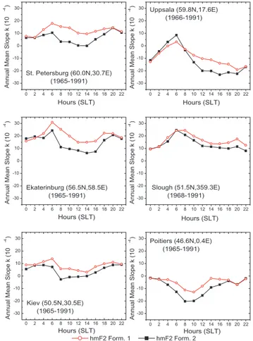
Fig. 2. Diurnal variation of thehmF2 trends when the Shimazaki (Formula 1) and the Dudeney (Formula 2) formulas were used to derivehmF2 fromM(3000)F2.
with
MF =M3{[(0.0196M32+1)/(1.2967M
2 3−1)]}
1/2
M3=M(3000)F2
and
1M=0.253/(r−1.215)−0.012
r=foF2/foE.
The results of such a comparison for St. Petersburg, Up-psala, Ekaterinburg, Slough, Kiev and Poitiers are shown in Fig. 2. All analysed stations demonstrate a systematic be-haviour of the trends when both formulas are applied; the trend magnitude tending slightly to decrease when the ef-fect of the underlying layer is taken into account by the ratio
foF2/foE (Formula 2). The differences in the trend magnitude are not very large and they depend on the local time. Both formulas give close results during nighttime hours whenfoE is small, but the difference increases during daytime hours when the E-layer contribution increases. Therefore, it should be kept in mind that hmF2 trend results are not as reli-able as foF2 ones because hmF2 values are inferred from
-20 -10 0 10 20 30 40
Slope K per year (10
-4
)
Slope K per year (10
-4
)
Slope K per year (10
-4
)
Slope K per year (10
-4
)
0 SLT (Model 1)
0 SLT (Model 1)
40 50 60 70 -20
-10 0 10 20 30 40
Geographic Latitude, deg
40 50 60 70
Geographic Latitude, deg
-20 -10 0 10 20 30 40
12 SLT (Model 1) 12 SLT (Model 2)
0 SLT (Model 2)
12 SLT (Model 2) 12 SLT (Model 1)
0 SLT (Model 2)
30 40 50 60 -20
-10 0 10 20 30 40
Geomagnetic Latitude, deg
30 40 50 60
Geomagnetic Latitude, deg
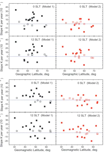
Fig. 3.A dependence of thehmF2 trend magnitude on geographic (top panel) and geomagnetic (bottom panel) latitude for two models, 00 and 12 SLT. Filled in symbols correspond to significant trends at a 95% confidence level. Note the absence of any pronounced dependence.
an additional noise to the analysedhmF2 values. There are some problems with the use of formula (2). It includes the
foF2/foE ratio, which should itself demonstrate long-term variations that distort the soughthmF2 trend. In addition,foE values used in the formula (2) are not available at many sta-tions during nighttime hours. Therefore, the simple formula by Shimazaki (1955) has been chosen for our analysis. This allowed us to analyse a greater number of ionosonde stations. In this context it should be mentioned that the use of model
foE values instead of absentfoE observations (Upadhyai and Mahajan, 1998) should distort thehmF2 trends asfoE itself demonstrates a long-term trend (Givishvili and Leshchenko, 1995; Bremer, 1998) which is not reflected by an empirical model such as IRI-90.
4 CalculatedhmF2 trends
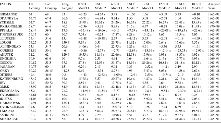
Ground-based ionosonde observations on 27 Eurasian sta-tions located in the 37◦N – 69◦N and 5.6◦W – 136◦E sector are used in this study. The list of the stations is given in
Ta--20 -10 0 10 20 30 40
12 SLT (Model 2) 0 SLT (Model 2)
12 SLT (Model 1) 0 SLT (Model 1)
0 20 40 60 80 100 120 140 -20
-10 0 10 20 30 40
Slope K per year (10
-4
)
Geographic Longitude, deg
Slope K per year (10
-4
)
0 20 40 60 80 100 120 140
Geographic Longitude, deg
Fig. 4.Same as Fig. 3 but for the dependence on geographic longi-tude. Note some longitudinal effect with negative trends at western European stations.
ble 2. The observations from most of them are seen to over-lap the analysed period of 1965–1991, which corresponds to the period of increasing geomagnetic activity. Moreover, this time period is the richest, with observations over the world-wide ionosonde network.
The calculatedhmF2 linear trends for four SLT moments (0, 6, 12 and 18) and two models are shown in Table 2. An inclusion of the dependence onAp12 to the regression
(Model 2) makes the trends more negative, while Model 1 provides more positive trend magnitudes. Mikhailov and Marin (2000) found the opposite effect of taking into account the dependence on theAp index for thefoF2 trends which were more positive in the latter case.
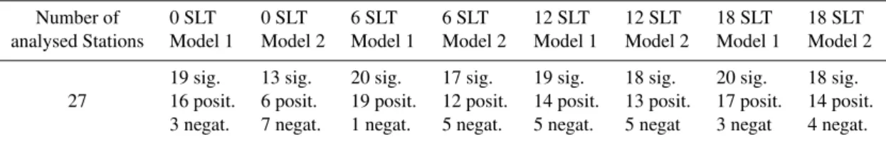
Most of the stations listed in Table 2 show significant trends. The number of stations with significant trends (neg-ative and positive) for four SLT moments and two models is summarised in Table 3. Most of them are seen to be pos-itive even when theAp index is included to the regression (Model 2). The only exception is for the 00 SLT (Model 2) case when the numbers of positive and negative significant trends are nearly the same. Therefore, the majority of the significanthmF2 trends are positive regardless of the model used. This is an important result of our analysis, which gives a clue for further physical interpretation.
Using the results given in Table 2, spatial (both latitudinal and longitudinal) variations of thehmF2 trends have been analysed. The slopes K at 00 and 12 SLT for the stations with observations available for the whole period 1965–1991 are plotted versus latitude (geomagnetic and geographic) and geographic longitude in Figs. 3 and 4, respectively. Regres-sions of hmF2 with R12 (Model 1) and with R12 +Ap12
(Model 2) are used in both figures for a comparison. The scatter of the slopeK at the analysed stations is seen to be smaller when theAp12 index is included to the regression
D.
Mar
in
et
al.:
L
ong-term
hm
F2
trend
s
765
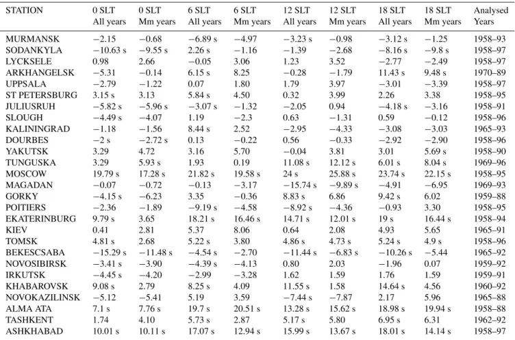
Table 2. Ionosonde stations and calculated annual mean slopeK(in 10−4units) for the period 1965–1991. Regression ofhmF2 withR12
(Model 1) and withR12+Ap12(Model 2), and all years in the indicated period are used to obtainhmF2 linear trends. Significant trends at
a confidence level of 95% are denoted by an “s” after the value
STATION Lat. Lat. Long. 0 SLT 0 SLT 6 SLT 6 SLT 12 SLT 12 SLT 18 SLT 18 SLT Analysed
Geomag. Geograp. Geograp. Model 1 Model 2 Model 1 Model 2 Model 1 Model 2 Model 1 Model 2 Years
MURMANSK 64 69 33 −3.23 −4.63 s 3.48 −1.60 1.66 −3.09 3.43 −0.10 1965–91
SODANKYLA 63.73 67.4 26.6 −6.71 s −6.94 s 8.24 s 1.50 5.08 −2.58 1.04 −3.26 1965–91
LYCKSELE 62.7 64.7 18.8 18.98 s 10.62 s 24.26 s 16.65 s 25.22 s 16.29 s 22.41 s 15.95 s 1965–91
ARKHANGELSK 58.7 64.6 40.5 −2.36 −5.31 8.95 s 6.15 s 4.77 −0.28 15.08 s 11.43 s 1970–89
UPPSALA 58.44 59.8 17.6 −15.49 s −19.06 s −0.11 −7.29 s −13.42 s −20.08 s −19.85 s −23.6 s 1965–91
ST PETERSBURG 56.17 60 30.7 7.64 s −0.23 17.87 s 8.28 s 10.12 s 3.67 13.54 s 7.05 1965–91
JULIUSRUH 54.4 54.6 13.4 −3.48 −10.38 s 2.67 −4.42 s 3.63 −2.08 −0.19 −4.69 s 1965–91
SLOUGH 54.25 51.5 359.4 9.19 s 0.51 23.78 s 11.92 s 15.00 s 6.64 s 15.66 s 7.55 s 1965–91
KALININGRAD 53.1 54.7 20.6 14.06 s 0.44 22.75 s 9.23 s 4.91 −3.36 5.55 −1.91 1965–91
DOURBES 51.89 50.1 4.6 −0.86 −2.77 s −2.71 −2.89 s −13.36 s −12.14 s −23.75 s −12.95 s 1965–91
YAKUTSK 51.2 62 129.6 19.55 s 11.16 s 22.66 s 12.58 s 15.96 s 6.93 s 18.37 s 9.92 s 1965–90
TUNGUSKA 50.9 61.6 90 9.7 s 2.53 4.64 0.64 16.64 s 9.15 s 12.77 s 6.95 s 1969–91
MOSCOW 50.82 55.5 37.3 27.8 s 12.07 s 31.87 s 18.19 s 29.26 s 16.82 s 31.18 s 18.12 s 1965–91
MAGADAN 50.75 60 151 9.29 s 2.15 9.02 0.35 −9.52 s −14.2 s 3.19 2.90 1969–91
GORKY 50.29 56.15 44.28 0.69 −3.34 8.77 s 4.95 15.47 s 8.03 s 14.58 s 9.67 s 1965–88
POITIERS 49.4 46.6 0.3 −4.43 −12.63 s −6.09 s −12.9 s −7.59 s −10.74 s −2.19 −5.75 1965–91
EKATERINBURG 48.42 56.4 58.6 15.75 s 5.57 30.87 s 19.6 s 14.87 s 9.21 s 22.15 s 14.61 s 1965–91
KIEV 47.5 50.72 30.3 8.89 s 0.41 13.75 s 5.37 4.35 0.64 9.82 s 4.93 1965–91
TOMSK 45.92 56.5 84.9 23.45 s 12.17 s 22.48 s 11.17 s 23.17 s 14.19 s 21.26 s 12.64 s 1965–91
BEKESCSABA 45.2 46.7 21.2 −11.94 s −13.54 s −3.77 −6.61 s −9.8 s −9.84 s −9.39 s −8.73 s 1965–91
NOVOSIBIRSK 44.61 54.6 83.2 7.96 s −0.06 8.17 s −0.15 7.59 s 1.17 6.2 s 0.28 1965–91
IRKUTSK 41.06 52.5 104 11.13 s 2.96 17.43 s 7.68 s 15.92 s 8.41 s 16.62 s 9.03 s 1965–91
KHABAROVSK 37.91 48.5 135.1 10.27 s 4.50 22.89 s 7.67 13.48 s 7.69 s 14.63 s 7.88 s 1965–91
NOVOKAZILINSK 37.6 45.77 62.12 1.44 −5.12 15.07 s 5.19 −0.97 −7.44 6.39 2.17 1965–88
ALMA ATA 33.42 43.2 76.9 12.51 s 5.64 s 28.27 s 20.84 s 18.77 s 16.31 s 22.98 s 19.55 s 1965–88
TASHKENT 32.3 41.33 69.62 4.99 2.29 10.98 s 6.51 3.97 5.17 s 9.37 s 8.01 s 1965–91
0 2 4 6 8 10 12 14 16 18 20 22 -30
-20 -10 0 10 20 30
Slope k (10
-4
)
Slope k (10
-4
)
Φ = (30-41N) Φ = (44-51N)
Geographic Longitude: 26-33E, degrees Geographic Longitude: 0-22E, degrees
Uppsala Slough Juliusruh Lycksele
Hours (SLT)
Slope k (10
-4
)
0 2 4 6 8 10 12 14 16 18 20 22 Bekescaba Dourbes Poitiers Kaliningrad
Hours (SLT)
0 2 4 6 8 10 12 14 16 18 20 22 -30
-20 -10 0 10 20 30
Φ = (45-53N) Φ = (54-62N)
Sokankyla Murmansk
Hours (SLT)
0 2 4 6 8 10 12 14 16 18 20 22 Φ = (63-64N)
Geographic Longitude: >37E, degrees St. Petersburg Kiev
Hours (SLT)
0 2 4 6 8 10 12 14 16 18 20 22 -30
-20 -10 0 10 20 30
Moscow Tomsk Ekaterinburg Novosibirsk
Hours (SLT)
0 2 4 6 8 10 12 14 16 18 20 22 Φ = (47-56N)
Irkutsk Tashken Khabarov Ashkhaba
Hours (SLT)
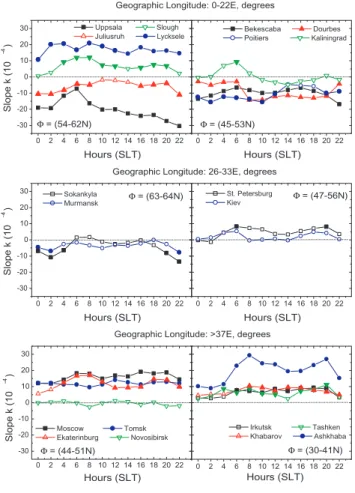
Fig. 5. Diurnal variation of thehmF2 trends in three longitudinal sectors. Regression ofhmF2 withR12+Ap12(Model 2) was used.
Filled in symbols correspond to significant trends at a 95% confi-dence level. The interval of geomagnetic latitudes8where stations are located is given in the plots.
latitudinal dependence was revealed for the foF2 trends (Danilov and Mikhailov, 1999; Mikhailov and Marin, 2000). This is another interesting result of our analysis which should be reconciled with the previous conclusions on the foF2 trends. On the other hand, some longitudinal effect is seen in Fig. 4. The trends have a tendency to have different signs in the West European and in the East European/Asian longi-tudinal sectors.
All negative trends are observed at the stations located be-tween 0 and 33◦E, while significant positive trends are ob-served to the east from 33◦E. But it should be pointed out that some stations, such as Slough or Lycksele, demonstrate significant positive trends and they are located in the West European longitudinal sector.
To study this effect in more detail, the diurnal variation of the trends has been calculated for all ionosonde stations shown in Fig. 4 (those ones with available observations for the period 1965–1991) using Model 2. The results are pre-sented in Fig. 5. Stations have been separated according to their longitude. Whereas most of the analysed stations lo-cated in the 0–22◦E longitudinal sector have negative trends (Fig. 5, top), those withλ > 37◦E (bottom panel) present
significant positive trends for all SLT. Stations in the bound-ary region (middle panel) show small positive or negative trends which are not significant. A similar longitudinal effect was found earlier by Bremer (1998). It should be stressed that although we observe some stations with significant neg-ative trends (all located in a small longitudinal sector of west-ern Europe), they are a minority as most of the stations are seen to present positive trends (see Tables 2 and 3). This longitudinal effect also requires physical interpretation.
Another point which should be taken into account in the long-term trends analysis is the possible influence of the hysteresis effect. Similar to foF2, the M(3000)F2 values also demonstrate a hysteresis effect in their solar cycle vari-ations (Rao and Rao, 1969). AshmF2 values are derived fromM(3000)F2, some effect may also be expected in the
hmF2 variations as well. Danilov and Mikhailov (1999) and Mikhailov and Marin (2000) found in theirfoF2 long-term trends research that only when the hysteresis effect at the rising and falling phases of a solar cycle was avoided, was it possible to obtain stable significant trends. They recom-mended using a selection of years around solar cycle maxi-mum and minimaxi-mum for thefoF2 trends analysis. Taking into account this result, we have tried to check the effect of the year selection on the resultanthmF2 trends. By analogy with the foF2 trends analysis, we considered all years and then only years around the solar cycle extrema. The results of this comparison are given in Table 4 (Model 1) and in Table 5 (Model 2). The selection of years applied in this analysis is based on the observed annual meanR12variations. Two or
three years around solar cycle maxima (M) and minima (m) with close annual meanR12values are selected for each solar
cycle (Table 1). As it can be seen from Tables 4 and 5, al-though there are some small differences in thehmF2 slopes for the two selections of years, the character of the trends does not change. Therefore, this (M)+(m) selection of years does not help to revealhmF2 trends, as it did in the case of thefoF2 trends. There is still no explanation for this result. Therefore, to revealhmF2 long-term trends, all years with available observations are used (as done in Table 2) since this increases the statistics and the confidence of results obtained.
5 Discussion
The physical mechanism of the ionospheric trends remains still unclear. Although the thermosphere cooling due to an increase in the atmospheric greenhouse gases has been pro-posed by different researchers as an explanation for hmF2 long-term trends, the results of the F2-layer parameter trends analysis cannot be explained by this greenhouse hypothesis. Global cooling of the upper atmosphere due to this effect would result in a negativehmF2 trend (Bremer, 1992; Ulich and Turunen, 1997) and a positive one infoF2 at least for the midlatitude F2-layer (Mikhailov and Marin, 2000), which is contrary to the obtained observations. This conclusion was obtained for the Northern Hemisphere stations. Long-term
Ar-D. Marin et al.: Long-termhmF2 trends 767
Table 3. Number of stations with significant (positive and negative)hmF2 trends taking into account the results presented in Table 2. Confidence level of 95% is applied
Number of 0 SLT 0 SLT 6 SLT 6 SLT 12 SLT 12 SLT 18 SLT 18 SLT analysed Stations Model 1 Model 2 Model 1 Model 2 Model 1 Model 2 Model 1 Model 2
19 sig. 13 sig. 20 sig. 17 sig. 19 sig. 18 sig. 20 sig. 18 sig. 27 16 posit. 6 posit. 19 posit. 12 posit. 14 posit. 13 posit. 17 posit. 14 posit.
3 negat. 7 negat. 1 negat. 5 negat. 5 negat. 5 negat 3 negat 4 negat.
Table 4.Calculated annual mean slope K (in 10–4 units) for the period 1965–1991. Regression ofhmF2 withR12(Model 1), and all years
as well as years around solar maximum and minimum (Mm years) are used to obtainhmF2 linear trends. Significant trends at a confidence level of 95% are denoted by an “s” after the value
STATION 0 SLT 0 SLT 6 SLT 6 SLT 12 SLT 12 SLT 18 SLT 18 SLT Analysed
All years Mm years All years Mm years All years Mm years All years Mm years Years
MURMANSK −3.23 1.00 3.48 1.56 1.66 4.38 3.43 3.02 1965–91
SODANKYLA −6.71 s −10.03 s 8.24 s 6.43 s 5.08 5.75 1.04 0.48 1965–91 LYCKSELE 18.98 s 20.27 s 24.26 s 24.85 s 25.22 s 30.6 s 22.41 s 23.11 s 1965–91 ARKHANGELSK −2.36 5.39 8.95 s 13.46 s 4.77 7.56 15.08 s 16.37 s 1970–89 UPPSALA −15.49 s −8.67 −0.11 3.53 −13.42 s −7.68 −19.85 s −16.08 s 1965–91 ST PETERSBURG 7.64 s 11.23 s 17.87 s 15.84 s 10.12 s 13.03 s 13.54 s 13.71 s 1965–91
JULIUSRUH −3.48 0.33 2.67 4.94 3.63 8.23 s −0.19 2.95 1965–91
SLOUGH 9.19 s 13.05 s 23.78 s 22.55 s 15.00 s 15.46 s 15.66 s 18.56 s 1965–91 KALININGRAD 14.06 s 14.07 s 22.75 s 17.98 s 4.91 5.10 5.55 5.46 1965–91 DOURBES −0.86 −1.01 −2.71 −1.23 −13.36 s −6.26 s −23.75 s −19.91 s 1965–91 YAKUTSK 19.55 s 16.8 s 22.66 s 18.19 s 15.96 s 16.41 s 18.37 s 16.97 s 1965–90 TUNGUSKA 9.7 s 13.08 s 4.64 3.76 16.64 s 19.02 s 12.77 s 13.79 s 1969–91 MOSCOW 27.8 s 36.89 s 31.87 s 40.79 s 29.26 s 42.6 s 31.18 s 41.81s 1965–91
MAGADAN 9.29 s 10.42 s 9.02 10.39 s −9.52 s −2.63 3.19 2.54 1969–91
GORKY 0.69 2.29 8.77 s 7.01 15.47 s 16.7 s 14.58 s 15.35 s 1965–88
POITIERS −4.43 −0.71 −6.09 s −2.34 −7.59 s −2.00 −2.19 7.19 1965–91 EKATERINBURG 15.75 s 16.84 s 30.87 s 32.35 s 14.87 s 18.29 s 22.15 s 25.2 s 1965–91
KIEV 8.89 s 12.58 s 13.75 s 17.69 s 4.35 6.35 9.82 s 11.24 s 1965–91
TOMSK 23.45 s 20.01 s 22.48 s 19.26 s 23.17 s 22.37 s 21.26 s 20.27 s 1965–91 BEKESCSABA −11.94 s −9.58 s −3.77 0.58 −9.8 s −6.77 s −9.39 s −6.23 s 1965–91 NOVOSIBIRSK 7.96 s 9.78 s 8.17 s 7.80 7.59 s 12.06 s 6.2 s 9.6 s 1965–91 IRKUTSK 11.13 s 8.54 s 17.43 s 10.74 s 15.92 s 12.01 s 16.62 s 11.32 s 1965–91 KHABAROVSK 10.27 s 10.93 s 22.89 s 2.77 s 13.48 s 7.66 s 14.63 s 12.48 s 1965–91 NOVOKAZILINSK 1.44 1.38 15.07 s 13.72 −0.97 −1.10 6.39 10.27 1965–88 ALMA ATA 12.51 s 15.12 s 28.27 s 29.71 s 18.77 s 20.99 s 22.98 s 25.81 s 1965–88
TASHKENT 4.99 5.93 10.98 s 5.52 3.97 3.02 9.37 s 6.53 1965–91
ASHKHABAD 33.41 s 32.32 s 40.78 s 37.79 s 35.22 s 35.04 s 41.44 s 41.35 s 1965–91
gentine Islands and Port Stanley were analysed by Jarvis et al. (1998) and for the Concepcion station by Foppiano et al (1999). Primarily negativehmF2 trends were revealed at these stations, especially for Port Stanley. ThehmF2 obser-vations from the first two stations were analysed by Danilov and Mikhailov (2001) using the same approach applied in this paper to reveal the trends. The Argentine Islands data are shown to demonstrate primarily positivehmF2 trends simi-lar to most of the Northern Hemisphere stations, whereas at Port Stanley, there is a stable negativehmF2 trend around the clock. It was concluded that the difference might be due to the fact that Port Stanley is close to the region of the South-Atlantic Geomagnetic Anomaly where processes
of direct corpuscular ionisation may play some role in the F2 layer formation thus disturbing the “normal” picture of
Fop-Table 5.Calculated annual mean slopeK(in 10−4units) for the whole period withhmF2 observations available on a particular ionosonde station. Regression ofhmF2 withR12+Ap12(Model 2) , and all years as well as years around solar maximum and minimum (Mm years)
are used to obtainhmF2 linear trends. Significant trends at a confidence level of 95% are denoted by an “s” after the value
STATION 0 SLT 0 SLT 6 SLT 6 SLT 12 SLT 12 SLT 18 SLT 18 SLT Analysed
All years Mm years All years Mm years All years Mm years All years Mm years Years
MURMANSK −2.15 −0.68 −6.89 s −4.97 −3.23 s −0.98 −3.12 s −1.25 1958–93 SODANKYLA −10.63 s −9.55 s 2.26 s −1.16 −1.39 −2.68 −8.16 s −9.8 s 1958–97
LYCKSELE 0.98 2.66 −0.05 3.06 1.23 3.52 −2.77 −2.49 1958–97
ARKHANGELSK −5.31 −0.14 6.15 s 8.25 −0.28 −1.79 11.43 s 9.48 s 1970–89
UPPSALA −2.79 −1.22 0.07 1.80 1.79 3.97 −3.01 −3.39 1958–97
ST PETERSBURG 3.15 s 3.13 5.84 s 4.50 0.32 3.99 2.26 3.38 1958–95
JULIUSRUH −5.82 s −5.96 s −3.07 s −1.32 −2.05 0.94 −4.18 s −3.16 1958–91
SLOUGH −4.49 s −4.07 1.19 −2.3 0.63 −1.31 0.59 −0.12 1958–96
KALININGRAD −1.18 −1.56 8.44 s 2.52 −2.95 −4.33 −3.08 −3.03 1965–93
DOURBES −2 s −2.72 s 0.13 −0.22 0.56 −0.33 −2.92 −2.90 1958–96
YAKUTSK 3.29 4.72 3.16 5.70 −0.04 3.81 3.01 5.69 s 1958–90
TUNGUSKA 3.29 5.93 s 1.93 0.19 11.08 s 12.12 s 6.01 s 8.04 s 1969–96
MOSCOW 19.79 s 17.28 s 21.82 s 19.58 s 24 s 25.88 s 23.74 s 22.15 s 1958–95 MAGADAN −0.07 −0.72 −0.13 −3.17 −15.74 s −9.89 s −4.91 −6.95 1969–93
GORKY −4.15 s −6.23 3.35 −0.36 8.83 s 6.86 9.42 s 6.02 1959–88
POITIERS −2.36 −1.89 −9.19 s −4.58 −8.92 s −4.36 −0.93 3.30 1958–95 EKATERINBURG 9.79 s 3.65 18.21 s 16.46 s 14.71 s 12.01 s 19 s 16.44 s 1958–94
KIEV 0.41 2.81 5.37 8.06 0.64 2.08 4.93 5.65 1965–91
TOMSK 4.81 s 2.68 5.22 s 3.80 4.86 s 4.73 s 5.24 s 4.9 s 1958–96
BEKESCSABA −15.29 s −11.48 s −4.54 s −2.70 −11.44 s −6.83 s −10.26 s −5.44 1965–92 NOVOSIBIRSK −3.41 s −3.90 −4.39 s −4.13 0.80 2.03 −1.96 0.07 1959–92
IRKUTSK −4.45 s −4.20 −2.99 −3.28 1.62 1.59 1.76 1.59 1959–91
KHABAROVSK 9.08 s 2.79 8.25 s 4.09 11.55 s 1.58 14.64 s 4.56 1960–92
NOVOKAZILINSK −5.12 −5.41 5.19 3.59 −7.44 s −7.87 2.17 5.96 1965–88 ALMA ATA 7.1 s 7.76 s 19.7 s 20.51 s 13.28 s 15.62 s 18.98 s 19.94 s 1958–88
TASHKENT 1.74 4.10 5.73 s 2.87 5.17 s 5.80 6.95 s 6.31 1962–92
ASHKHABAD 10.01 s 10.11 s 17.07 s 12.94 s 15.99 s 13.67 s 18.01 s 14.14 s 1958–97
piano et al. (1999) have analysed all available (1958–1994) observations which belong to different periods in the geo-magnetic activity long-term variation and this cannot be ig-nored in the F2-layer parameters trend analysis (Mikhailov and Marin, 2000, 2001). In addition, it should be stressed that mechanisms of F2-layer trends are different at low, mid-dle and high-latitude stations, reflecting the specificity of the F2-layer formation and they can hardly be attributed just to the thermosphere cooling due to the greenhouse effect.
In connection with this discussion it is interesting to con-sider the results by Keating et al. (2000) who, in analysing the orbits of 5 satellites, found a 9.8±2.5% decrease in the total thermospheric densityρat 350 km in 1996 with respect to 1976. They attribute this effect to a 10% increase in the atmospheric CO2 abundance. According to their estimates,
such a 10% decrease inρshould result in a 5 km lowering of the constant pressure level. This seems to be in line with the
hmF2 long-term decrease which many researchers are look-ing for. The Keatlook-ing et al. (2000) results may be consid-ered as the first and the only direct experimental evidence for long-term changes in the thermosphere presumably related with the greenhouse thermosphere cooling hypothesis. But one should keep in mind that such small (less than 10% over
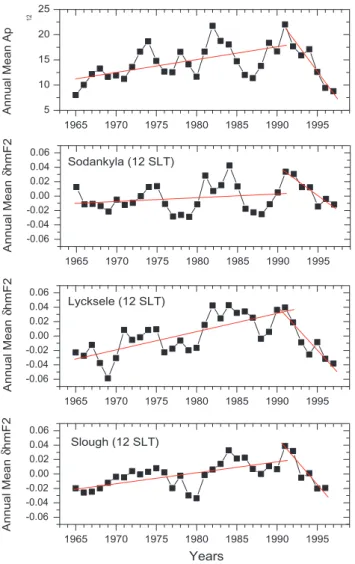
20 years) changes inρ may be due to some other reasons, such as: the conversion of orbital data to atmospheric den-sity, the accuracy of the empirical model MET99 used for the data reduction. Unfortunately ionospheric F2layer observa-tions cannot help us to reveal such small changes inρwhich (if they really exist) are masked by stronger processes. On the other hand, according to the geomagnetic control con-cept by Mikhailov and Marin (2000), the 1996 belongs to the period of decreasing geomagnetic activity (1990-91 is a turning point), therefore one should expect negative hmF2 trend at mid-latitudes after 1991 which is due to a decrease in geomagnetic activity but not to a greenhouse effect. Some examples of such change in thehmF2 trends after 1991 are given in Fig. 6.
an-D. Marin et al.: Long-termhmF2 trends 769 other turning point). Therefore, trends should be analysed
over a time interval which does not include different (in-creasing/decreasing) periods in geomagnetic activity. This was the reason for analysing thehmF2 trends for the time period 1965–1991 with the increasing geomagnetic activity. Such proposed geomagnetic control of thefoF2 trends im-plies corresponding trends inhmF2. So let us analysehmF2 trends from this point of view. An approximate expression for hmF2 can be written for the day-time mid-latitude F2-region according to Ivanov-Kholodny and Mikhailov (1986):
hm∼=
H
3 {ln[O]1+lnβ1+ln(H
2/
0.54d)} +cW, (2) whereH =kTn/mgis the scale height and [O] is the con-centration of atomic oxygen,β is the linear loss coefficient at a fixed heighth1,W (in m/s) is the vertical plasma drift
which is primarily related to thermospheric winds,cis a co-efficient close to unity,d=1.38∗1019∗(Tn/1000)0.5is a co-efficient in the expression for the ambipolar diffusion coeffi-cientD=d/[O]. The loss coefficientβdepends on the den-sity of the molecular gases N2and O2:β=k1[N2] +k2[O2],
where k1 andk2 are the reaction rate constants of the two
processes controlling the sink of O+ions in the F2-region: O++N2
k1
−→NO++N; O++O2
k2
−→O+2 +O both rate constants being temperature dependent (Hierl et al., 1997).
The main processes responsible for the F2-layer storm effects are known: neutral composition, temperature and thermospheric wind changes at middle and lower latitudes, while electric fields and particle precipitation strongly af-fect the high-latitude F2-region (Pr¨olss, 1995, and references therein). During geomagnetic disturbed periods, the high-latitude energy inputs (Joule heating and particle precipita-tion) cause changes in the thermosphere global circulation. These result in a perturbation of neutral composition and temperature, with a decrease in [O] and an increase in [N2],
[O2] and neutral temperature. Such perturbations are
be-lieved to be the main reason for the mid-latitude F2-region negative storm effect. They result in an increase of the linear loss coefficientβ (due to the N2and O2concentrations and
temperature increase) with a correspondinghmF2 increase. The decrease in atomic oxygen concentration has an opposite effect onhmF2, but the effect of aβincrease usually prevails (Mikhailov and F¨orster, 1997, 1999). Therefore, we should expect positivehmF2 trends at middle latitudes as a reaction to an increase in geomagnetic activity.
At lower latitudes, neutral composition variations are not large (e.g. Pr¨olss, 1995 and references therein) and the usual observed positive F2-layer storm effects are primarily due to an increase in the equatorward thermospheric wind. Some contribution to the F2-layer positive storm effects at lower latitudes provides atomic oxygen (Mikhailov et al. 1995). This results in small or even positive foF2 trends at lower latitudes, as was shown by Mikhailov and Marin (2000) and should result in positivehmF2 trends as well. As both mech-anisms work in one direction (hmF2 increase), changing
1965 1970 1975 1980 1985 1990 1995 -0.06
-0.04 -0.02 0.00 0.02 0.04 0.06
Slough (12 SLT) Lycksele (12 SLT)
Years
1965 1970 1975 1980 1985 1990 1995 -0.06
-0.04 -0.02 0.00 0.02 0.04 0.06
1965 1970 1975 1980 1985 1990 1995 -0.06
-0.04 -0.02 0.00 0.02 0.04 0.06
Annual Mean
δ
hmF2
Annual Mean
δ
hmF2
Annual Mean
δ
hmF2 Sodankyla (12 SLT)
1965 1970 1975 1980 1985 1990 1995 5
10 15 20 25
Annual Mean Ap
12
Fig. 6. Annual meanAp12 and δhmF2 variations at Sodankyla, Lycksele and Slough, and 12 SLT (Model 1). Note different signs of trends for the period prior and after 1991.
each other as we pass from middle to lower latitudes, one should not expect any pronounced latitudinal dependence in
hmF2 trends, as it was shown by our analysis. Therefore, the revealed positivehmF2 trends from the majority of the stations can be explained by the F2-layer storm mechanism due to the long-term increase in geomagnetic activity which takes place after 1965.
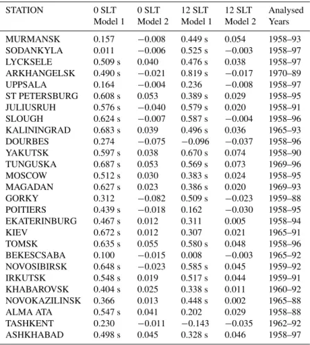
Table 6.Calculated coefficients of correlation r between annual meanhmF2 andAp12values for the whole period withhmF2 observations
available on a particular ionosonde station. Regression ofhmF2 withR12(Model 1) and withR12+Ap12(Model 2), and all years in the
indicated period are used to obtain the coefficients. Significant coefficients at a confidence level of 95% are denoted by “s” after the value
STATION 0 SLT 0 SLT 12 SLT 12 SLT Analysed Model 1 Model 2 Model 1 Model 2 Years
MURMANSK 0.157 −0.008 0.449 s 0.054 1958–93 SODANKYLA 0.011 −0.006 0.525 s −0.003 1958–97 LYCKSELE 0.509 s 0.040 0.476 s 0.038 1958–97 ARKHANGELSK 0.490 s −0.021 0.819 s −0.017 1970–89 UPPSALA 0.164 −0.004 0.236 −0.008 1958–97 ST PETERSBURG 0.608 s 0.053 0.389 s 0.029 1958–95 JULIUSRUH 0.576 s −0.040 0.579 s 0.020 1958–91 SLOUGH 0.624 s −0.007 0.587 s −0.004 1958–96 KALININGRAD 0.683 s 0.039 0.496 s 0.036 1965–93 DOURBES 0.274 −0.075 −0.096 −0.037 1958–96 YAKUTSK 0.597 s 0.038 0.670 s 0.074 1958–90 TUNGUSKA 0.687 s 0.053 0.569 s 0.073 1969–96 MOSCOW 0.512 s 0.030 0.383 s 0.024 1958–95 MAGADAN 0.627 s 0.023 0.386 s 0.020 1969–93 GORKY 0.312 −0.082 0.509 s −0.023 1959–88 POITIERS 0.439 s −0.018 0.162 −0.030 1958–95 EKATERINBURG 0.467 s 0.012 0.311 0.005 1958–94
KIEV 0.672 s 0.012 0.307 0.021 1965–91
TOMSK 0.635 s 0.055 0.580 s 0.048 1958–96 BEKESCSABA 0.100 −0.015 0.008 −0.003 1965–92 NOVOSIBIRSK 0.648 s −0.023 0.585 s 0.045 1959–92 IRKUTSK 0.548 s 0.019 0.517 s 0.044 1959–91 KHABAROVSK 0.404 s 0.025 0.338 s 0.011 1960–92 NOVOKAZILINSK 0.366 0.013 0.448 s 0.002 1965–88 ALMA ATA 0.547 s 0.041 0.202 0.029 1958–88 TASHKENT 0.230 −0.011 −0.143 −0.035 1962–92 ASHKHABAD 0.498 s 0.045 0.328 s 0.046 1958–97
An example of this fact can be observed when comparing Lycksele and Uppsala ionosonde stations. These stations are pretty close (see Table 2), but they demonstrate significant trends of different signs. Nonetheless, positivehmF2 trends obtained for most of the stations analysed may be considered as serious support for the geomagnetic origin of the F2-layer parameter long-term trends.
Finally, in order to test the proposed relationship between thehmF2 trends and geomagnetic activity, we calculated the correlation coefficients between the annual meanδhmF2 and theAp12 for each ionosonde station, using the whole period
with observations available. The results of this analysis are given in Table 6. All analysed stations demonstrate posi-tiveδhmF2–Ap12 correlation, with most of them (19 of 27
both at 00 and 12 SLT) being significant with a confidence level of 95% when Model 1 is used. Such correlation disap-pears when a geomagnetic index is included to the regression (Model 2) and this is not surprising. The obtained positive correlation (when Model 1 is used) may be considered as a clear indication of the relationship betweenhmF2 trends and geomagnetic activity. However, it should be pointed out that despite the fact that theδhmF2–Ap12correlation disappears
whenAp12is taken into account in the regression (Model 2),
the inclusion of this index, in fact, does not remove the geo-magnetic effects on the trends (Mikhailov and Marin, 2000, 2001). Although there is an obvious relationship between the F2-layer parameter trends and the geomagnetic activity, it is impossible to remove this geomagnetic effect from the trends revealed using any conventional index (e.g. monthly or annual mean Ap) of geomagnetic activity. If it could be done using the conventional indices, the problem of the F2-layer storm description and prediction would have been solved long ago, but this is not the case up until now. This is not surprising as any global geomagnetic activity index cannot, in principle, take into account the whole complexity of F2-layer storm effects with positive and negative phases depending on season, UT and LT of storm onset, storm mag-nitude, etc. Indeed, the inclusion ofAp12 to the regression
(Model 2) has some effect on the trend magnitude, but with-out changing, in principle, the results obtained whenAp12
D. Marin et al.: Long-termhmF2 trends 771 F2-layer storm mechanisms. On the other hand an additional
analysis is required to find out the reason for significant neg-ativehmF2 trends revealed at some stations.
6 Conclusions
The main results of this analysis may be listed as follows: 1. The new approach proposed by Danilov and Mikhailov (1998, 1999) and Mikhailov and Marin (2000) has been used to revealhmF2 linear trends at 27 European and Asian ionosonde stations. Although the choice of a simple formula by Shimazaki (1955) for thehmF2 derivation has no princi-ple influence on the trends obtained during nighttime hours, the trends turn out to be slightly less if the effect of underly-ing ionisation is taken into account by applyunderly-ing more accu-rate formulas during daytime hours.
2. The majority of the stations show significant posi-tive trends for the period of increasing geomagnetic activ-ity 1965–1991, without any dependence on latitude (neither magnetic nor geographic). This result can be explained in the framework of the long-term increase in geomagnetic activity and related F2-layer storm activity. The significant positive correlation obtained between the annualδhmF2 and Ap12
values confirms this close relationship betweenhmF2 trends and geomagnetic activity. However, some stations located in the western part of Europe demonstrate significant negative trends. This longitudinal effect (earlier revealed by Bremer) needs further analysis as significant negative trends observed at some western European stations are not explained within the geomagnetic control concept.
3. Unlike the case withfoF2 trends, a selection of years around solar cycle minimum and maximum does not help to revealhmF2 trends and using of all years with available ob-servations may be recommended for thehmF2 trends analy-sis. This increases the statistics and the confidence of results obtained.
4. Positive significanthmF2 trends obtained for the major-ity of the stations considered (regardless of the model used) contradict the suggestion that thermospheric cooling due to the greenhouse effect might be the cause of the F2-layer parameter trends. However, they can be explained in the framework of the geomagnetic control hypothesis proposed by Mikhailov and Marin (2000).
Acknowledgements. This work was in part supported by the Rus-sian foundation for Fundamental Research under Grant 00–05– 64189, and it has also been possible thanks to financial support granted by the National Institute of Aerospace Technology (INTA – Spain).
Topical Editor M. Lester thanks L. Cander and J. Lastovicka for their help in evaluating this paper.
References
Bilitza, D., Sheikh, N. M., and Eyrig, R., A global model for the height of the F2-peak using M3000 values from the CCIR nu-merical map, Telecom J., 46, 549–553, 1979.
Bradley, P. A. and Dudeney, J. R., A simple model of the vertical distribution of electron concentration in the ionosphere, J. Atm. Terr. Phys., 35, 2131–2146, 1973.
Bremer, J., Ionospheric trends in mid-latitudes as a possible indica-tor of the atmospheric greenhouse effect, J. Atmos. Terr. Phys., 54, 1505–1511, 1992.
Bremer, J., Trends in the ionospheric E and F regions over Europe, Ann. Geophys., 16, 986–996, 1998.
CCIR, Documents CCIR Study Group, Period 1986–1990, Geneva, 27 April – 10 May, Rec. 371–5, p. 47, 1988.
Danilov, A. D., Long-term changes of the mesosphere and lower thermosphere temperature and composition, Adv. Space Res., 20 (11), 2137–2147, 1997.
Danilov, A. D., Review of long-term trends in the upper meso-sphere, thermosphere and ionomeso-sphere, Adv. Space Res., 22 (6), 907–915, 1998.
Danilov, A. D. and Mikhailov, A. V., Long-term trends of the F2-layer critical frequencies: a new approach, Proceedings of the 2nd COST 251 Workshop “Algorithms and models for COST 251 Final Product”, 30–31 March, 1998, Side, Turkey, Ruther-ford Appleton Lab., UK, 114–121, 1998.
Danilov, A. D. and Mikhailov, A. V., Spatial and seasonal variations of thefoF2 long-term trends, Ann. Geophys., 17, 1239–1243, 1999.
Danilov, A. D. and Mikhailov, A. V., F2-layer parameters long-term trends on the Argentine Islands and Port Stanley vertical sound-ing data, (submitted to Ann. Geophys.) 2001.
Deminov, M. G., A. V. Garbatsevich, and R.G. Deminov, Climatic changes of the ionospheric F2-layer, Doklady RAN, 372 (3), 383–385, (in Russian) 2000.
Dudeney, J. R., Brit. Antarct. Surv. Sci. Rept 88, 1974.
Dudeney, J. R., An improved model of the variation of the elec-tron concentration with height in the ionosphere, J. Atmos. Terr. Phys., 40, 95–203, 1978.
Foppiano, A. J., Cid, L., and Jara, V., Ionospheric long-term trends for South American mid-latitudes, J. Atmos. Solar-Terr. Phys., 61, 717–723, 1999.
Givishvili, G. V. and Leshchenko, L. N., Possible proofs of presence of technogenic impact on the midlatitude ionosphere, Doklady RAN, 334 (2), 213–214, 1994 (in Russian).
Givishvili, G. V. and Leshchenko, L. N., Dynamics of the climatic trends in the midlatitude in the midlatitude ionospheric E region, Geomag. Aeronom., 35 (3), 166–173, (in Russian) 1995. Givishvili, G. V., Leshchenko, L. N., Shmeleva, O. P., and Ivanidze,
T. G., Climatic trends of the mid-latitude upper atmosphere and ionosphere, J. Atmos. Terr. Phys., 57, 871–874, 1995.
Hierl, P. M., Dotan, I., Seeley, J. V., Van Doran, J. M., Morris, R. A., and Viggiano, A. A., Rate coefficients for the reactions of O+ with N2 and O2 as a function of temperature (300–188 K), J. Chem. Phys., 106 (9), 3540–3544, 1997.
Ivanov-Kholodny, G. S. and Mikhailov, A. V., The prediction of ionospheric conditions, D. Reidel Publ. Co., Dordrecht, The Netherlands, 1986.
Jarvis, M. J., Jenkins, B., and Rodgers, G. A., Southern Hemisphere observations of a long-term decrease in F region altitude and thermospheric wind providing possible evidence for global ther-mospheric cooling, J. Geophys. Res., 103, 20774–20787, 1998. Keating, G. M., Tolson, R. H., and Bradford, M. S., Evidence of
long term global decline in the Earth’s thermospheric densities apparently related to anthropogenic effects, Geophys. Res. Lett., 27, 1523–1526, 2000.
F2-layer positive storm effect at middle and lower latitudes, Ann. Geophys., 13, 532–540, 1995.
Mikhailov, A. V., Mikhailov, V. V., and Skoblin, M. G., Monthly medianfoF2 andM(3000)F2 ionospheric model over Europe, Ann. Geophys., 39, 791–805, 1996.
Mikhailov, A. V. and F¨orster, M., Day-to-day thermosphere param-eter variation as deduced from Millstone Hill incoherent scatter radar observations during 16–22 March, 1990 magnetic storm period, Ann. Geophys., 15, 1429–1438, 1997.
Mikhailov, A. V. and F¨orster, M., Some F2-layer effects during the 6–11 January , 1997 CEDAR storm period as observed with the Millstone Hill incoherent scatter facility, J. Atmos. Solar-Terr. Phys., 61, 249–261, 1999.
Mikhailov, A. V. and Marin, D., Geomagnetic control of thefoF2 trends, Ann. Geophys., 18, 653–665, 2000.
Mikhailov, A. V. and Marin, D., An interpretation of thefoF2 and
hmF2 long-term trends in the framework of the geomagnetic control concept, Ann. Geophys., 19, 733–748, 2001.
Pollard, J. H., A handbook of numerical and statistical techniques, Camb. Univ. Press, 1977.
Pr¨olss, G. W., Ionospheric F region storms, in Handbook of Atmo-spheric Electrodynamics, 2, edited by H. Volland, pp. 195–248, CRC Press, Boca Raton, Fla., 1995.
Rao, M. S. V. G., and Rao, R. S., The hysteresis variation in F2-layer parameters, J.Atmos. Terr. Phys., 31, 1119–1125, 1969.
Rishbeth, H., A greenhouse effect in the ionosphere?, Planet. Space Sci., 38, 945–948, 1990.
Rishbeth, H. and Roble, R. G., Cooling of the upper atmosphere by enhanced greenhouse gases – modelling of thermospheric and ionospheric effects, Planet. Space Sci., 40, 1011–1026, 1992. Rishbeth, H., Long-term changes in the ionosphere, Adv. Space
Res., 20 (11) 2149–2155, 1997.
Roble, R. G. and Dickinson, R. E., How will changes in carbon dioxide and methane modify the mean structure of the meso-sphere and thermomeso-sphere, Geophys. Res. Lett. 16, 1441–1444, 1989.
Sharma, S. S., Chandra, H. and Vyas, G. D., Long-term ionospheric trends over Ahmedabad, Geophys. Res. Lett., 26, 433–436, 1999. Shimazaki, T., World-wide variations in the height of the maximum electron density of the ionospheric F2 layer, J. Radio Res. Labs. Japan, 2 (7), 85–97, 1955.
Ulich, T., How do long-term trends in F2 layer peak height depend on the underlying ionospheric model?, Paper presented at Ses-sion ST3 of the 25th EGS General Assembly, Nice, April, 2000. Ulich, T. and Turunen, E., Evidence for long-term cooling of the upper atmosphere in ionospheric data, Geophys. Res. Lett., 24, 1103–1106, 1997.