www.atmos-chem-phys.net/14/199/2014/ doi:10.5194/acp-14-199-2014
© Author(s) 2014. CC Attribution 3.0 License.
Atmospheric
Chemistry
and Physics
Field measurements of trace gases emitted by prescribed fires in
southeastern US pine forests using an open-path FTIR system
S. K. Akagi1, I. R. Burling1, A. Mendoza2, T. J. Johnson2, M. Cameron3, D. W. T. Griffith3, C. Paton-Walsh3, D. R. Weise4, J. Reardon5, and R. J. Yokelson1
1University of Montana, Department of Chemistry, Missoula, MT 59812, USA 2Pacific Northwest National Laboratories, Richland, WA 99354, USA
3University of Wollongong, Department of Chemistry, Wollongong, New South Wales, Australia
4USDA Forest Service, Pacific Southwest Research Station, Forest Fire Laboratory, Riverside, CA 92507, USA 5USDA Forest Service, Rocky Mountain Research Station, Fire Sciences Laboratory, Missoula, MT 59808, USA
Correspondence to:R. J. Yokelson (bob.yokelson@umontana.edu)
Received: 24 March 2013 – Published in Atmos. Chem. Phys. Discuss.: 10 July 2013 Revised: 22 October 2013 – Accepted: 23 October 2013 – Published: 8 January 2014
Abstract. We report trace-gas emission factors from three pine-understory prescribed fires in South Carolina, US mea-sured during the fall of 2011. The fires were more intense than many prescribed burns because the fuels included ma-ture pine stands not subjected to prescribed fire in decades that were lit following an extended drought. Emission fac-tors were measured with a fixed open-path Fourier transform infrared (OP-FTIR) system that was deployed on the fire con-trol lines. We compare these emission factors to those mea-sured with a roving, point sampling, land-based FTIR and an airborne FTIR deployed on the same fires. We also compare to emission factors measured by a similar OP-FTIR system deployed on savanna fires in Africa. The data suggest that the method used to sample smoke can strongly influence the relative abundance of the emissions that are observed. The majority of fire emissions were lofted in the convection col-umn and were sampled by the airborne FTIR. The roving, ground-based, point sampling FTIR measured the contribu-tion of individual residual smoldering combuscontribu-tion fuel ele-ments scattered throughout the burn site. The OP-FTIR pro-vided a∼30 m path-integrated sample of emissions
trans-ported to the fixed path via complex ground-level circula-tion. The OP-FTIR typically probed two distinct combustion regimes, “flaming-like” (immediately after adjacent ignition and before the adjacent plume achieved significant vertical development) and “smoldering-like.” These two regimes are denoted “early” and “late”, respectively. The path-integrated sample of the ground-level smoke layer adjacent to the fire
from the OP-FTIR provided our best estimate of fire-line ex-posure to smoke for wildland fire personnel. We provide a table of estimated fire-line exposures for numerous known air toxics based on synthesizing results from several studies. Our data suggest that peak exposures are more likely to chal-lenge permissible exposure limits for wildland fire personnel than shift-average (8 h) exposures.
1 Introduction
occurs when the majority of the smoke is produced by flam-ing combustion, lofted via convection, and directed away from major population centers. This requires that fuel con-ditions, boundary layer depth, wind speed, and wind direc-tion are within specific limits. Land managers try to mini-mize prolonged smoldering outside the envelope of convec-tion from the flame front. This type of combusconvec-tion is of-ten termed “residual smoldering combustion”, or RSC, and typically produces un-lofted smoke that accounts for many of the local-scale air quality impacts of prescribed burning (Bertschi et al., 2003; Achtemeier, 2006). There are very few peer-reviewed field measurements of the emissions from RSC (Bertschi et al., 2003; Burling et al., 2011; Akagi et al., 2013) and these measurements are becoming more de-sirable with increased recognition that RSC is a major fuel consumption process in some ecosystems (Christian et al., 2007; Greene et al., 2007; Hyde et al., 2011; Turetsky et al., 2011; Benscoter et al., 2011).
This work is part of a series of studies focusing on smoke emissions from prescribed fires on US Department of De-fense (DoD) bases. Previous studies from this series include Burling et al. (2010) who sampled the emissions from fu-els collected on bases that were burned in a large labora-tory combustion facility; Burling et al. (2011) and Akagi et al. (2012, 2013) who described airborne and ground-based smoke measurements on bases in the western and southeast-ern US; and Yokelson et al. (2013) who synthesized the lab-oratory and field results. In the previous studies, Burling et al. (2011) and Akagi et al. (2013) used a mobile, closed-cell FTIR system to search for and sample RSC point sources based on the observation of visible smoke plumes emanat-ing from specific smolderemanat-ing logs, stumps, litter, etc. In this study we focus on “passive” ground level emissions measure-ments using a static, open-path Fourier transform infrared (OP-FTIR) gas analyzer system that measured all smoke (in-cluding both flaming and smoldering emissions) that drifted through the fixed measurement path of∼30 m. Griffith et
al. (1991) was first to employ an OP-FTIR system to study biomass burning emissions. More recently, OP-FTIR has been used to study polluted air in challenging environmental or industrial conditions, such as measuring volcanic emis-sions or aircraft exhaust (Gosz et al., 1988; Oppenheimer and Kyle, 2007; Schäfer et al., 2005). Recently, Wooster et al. (2011) revived the use of OP-FTIR for field measurements of biomass burning, reporting emission ratios (ER) and emis-sion factors (EF) for CO2, CO, CH4, HCHO, and NH3from
savanna fires in Kruger National Park, South Africa. An important application of our open-path data is bet-ter understanding of the composition of ground-level smoke from prescribed burning to help minimize human exposure to potentially harmful toxins. Smoke could affect human health via numerous, complex, and poorly understood mechanisms. In particular, firefighters, burn managers, and other wild-land fire personnel are subjected to a complex mixture of combustion-generated gases and respirable particles. This
in-cludes at least five chemical groups classified as known hu-man carcinogens by the International Agency for Research on Cancer (IARC), other species classified by the IARC as probable or possible human carcinogens, and at least 26 chemicals listed by the US EPA as hazardous air pollutants (Naeher et al., 2007). Adverse health effects caused by smoke emitted during a fire could potentially include upper respi-ratory symptoms (Swiston, 2008), neurological symptoms, and cancer (though previous studies have not found a strong link between the two, Demers et al., 1994). Only a few stud-ies in the literature have evaluated occupational exposure to smoke among firefighters (Materna et al., 1992; Reinhardt and Ottmar, 1997, 2004; Adetona et al., 2011).
Measuring fire-line exposures to various toxins present in smoke for comparison to established exposure limits is not simple because fire intensity, fuel composition, and weather conditions are constantly changing and thereby modifying the smoke chemistry and dilution occurring in the work en-vironment (Sharkey, 1997). Different fire types also pose different conditions; several studies found that exposures to pollutants were higher among firefighters at prescribed fires than at wildfires (Reinhardt and Ottmar, 2004; Sharkey, 1997). In addition, smoke exposure can vary by work ac-tivity (e.g. direct attack, lighting, mop-up) (Reinhardt and Ottmar, 2004). For the typical morning prescribed burn, in-creasing afternoon winds may increase smoke distribution and risk of smoke overexposure for some workers. Vari-ous measurement techniques, including electronic dosime-ters, liquid chromatography, and gas chromatography/flame ionization detection (FID) have been employed to measure different species in smoke. This work is the first to assess fire-line exposure using the open-path FTIR technique.
In summary, this study first describes the OP-FTIR system employed on three Fort Jackson fires and the data reduction approach. We then present a time series of OP-FTIR results with the simultaneous observations of the other FTIR instru-ments noted for perspective. We calculate OP-FTIR EF for the trace gases detected and these EF are then compared to EF from the other FTIRs on the same fires and to EF mea-sured by an OP-FTIR system deployed on savanna fires. Fi-nally, we combine the OP-FTIR mixing ratio measurements on the fire-line with results from the other DoD studies to generate a preliminary assessment of fire-line exposure to air toxins.
2 Experimental details
2.1 Open-path FTIR measurements
species in the atmosphere across distances of tens to hun-dreds of meters. An active configuration was used with an unmodulated SiC glowbar source and sender telescope at one end of the light path and the FTIR with receiver tele-scope at the other. The source was powered (∼20 W) using
a 12.6 V DC automobile battery. The 1200◦C SiC source was mounted at the focal point of an F/4 Newtonian tele-scope with a 150 mm clear aperture. The sender teletele-scope directed a collimated, broadband IR beam to a 137 mm re-ceiver telescope coupled to the OPAG-22 FTIR spectrometer. Pathlengths of 29.3–32.2 m were used to optimize infrared intensity and sensitivity (Fig. 1b). On the receiving end, the OPAG-22 was powered by two automobile batteries in se-ries to provide∼25 V DC. The nominal field of view of the
spectrometer is 30 milliradians (mrad), which was reduced to 10 mrad by the F/3 receiver telescope (Fig. 1a). The in-terferometer uses dual retro-reflecting cube corner mirrors in an inverted pendulum mechanism that does not need align-ment in the field. The FTIR used a Stirling-cycle cooled mer-cury cadmium telluride (MCT) detector with a proprietary software correction for nonlinearity (Keens, 1990). Spectra were recorded at a resolution of 1.5 cm−1and 50 scans were co-added to give increased signal-to-noise ratio (SNR) at a time resolution of 134 s per spectrum. After aligning the tele-scopes, an ambient emission spectrum was recorded with the source turned off. This spectrum accounts for emission from the ambient-temperature environment which is modulated by the interferometer and detected in the FTIR spectra. The am-bient emission spectrum was subtracted from all measured globar spectra before further analysis.
The emission-corrected sample spectra were then ana-lyzed either directly as single-beam spectra, or as transmis-sion spectra ratioed to a background air spectrum taken be-fore the fire. Ratioing to background was used only in spec-tral regions where the continuum spectrum of the source-telescope-interferometer system was complex and could not be fitted well by the analysis procedure. The background spectrum was also used to characterize the composition of the pre-fire atmosphere. Analysis was by iterative non-linear least-squares fitting of the measured spectra by calculated spectra as described in previous work (Burling et al., 2011; Griffith et al., 2012). The calculated spectra are based on HITRAN (Rothman et al., 2009) and Pacific Northwest Na-tional Laboratory (Sharpe et al., 2004; Johnson et al., 2006, 2010) spectral databases, and include the effects of envi-ronmental pressure and temperature as well as the instru-ment line shape and resolution. Spectra were analyzed in domains of typically 10 to 200 cm−1 width, with each
re-gion targeting one or more trace gases (see Table A1 in Ap-pendix A for all species reported and the spectral analysis regions from which they were retrieved). Typical precision of measurements is < 1 % for dominant species such as CO2,
CO and CH4, but accuracy may be a few percent, varying
from species to species; Smith et al. (2011) provide a de-tailed analysis of the accuracy of OP-FTIR measurements.
Fig. 1. (a)Photograph of the OPAG-22 spectrometer system with
receiver telescope in the field during the 2 November fire.(b)
Pho-tograph of the sender and receiver telescopes separated by an
opti-cal path of∼30 m taken in clean air before ignition on 30 October.
(c)Photograph of the 2 November fire from the airborne platform
used by the airborne FTIR system. Pictures of fuels sampled by the LAFTIR can be found in Akagi et al. (2013).
Detection limits for trace species are typically 1–10 ppb. Ex-cess mixing ratios (EMRs) for any species X detected when smoke filled the optical path (denoted1X, the mixing ratio of species X in a smoke plume layer minus its mixing ratio in background air) were obtained directly from the transmission spectra or by difference between the appropriate single beam retrievals for H2O, CO2, CO, and CH4in the plume and
2.2 Other gas-phase sampling instruments
In addition to measurements made by the OP-FTIR, two closed-cell FTIR systems were employed: (1) an Airborne FTIR (AFTIR) to sample lofted fresh and photochemically aged smoke (Fig. 1c), and (2) a mobile, LAnd-based FTIR (LAFTIR) system to sample point sources of smoldering smoke (Akagi et al., 2013). This work will focus primarily on gas-phase species measured by the OPAG-22 (hereafter referred to as the OP-FTIR) system, but it is instructive to compare with the other FTIRs at times. Whole air sampling (WAS) canisters were also used on the ground and in the air to measure an extensive suite of gases (mostly non-methane organic compounds, NMOCs) and are reported in Akagi et al. (2013).
2.3 Calculation of emission ratios (ERs) and emission factors (EFs)
Excess mixing ratios for FTIR species were calculated fol-lowing the procedure in Sect. 2.1. The molar emission ratio (ER) is calculated by dividing1X by the EMR of a refer-ence species1Y, usually1CO or1CO2, measured in the
same fresh smoke sample as “X”. Since all species are re-trieved from the same spectrum at the same time, emission ratios can be determined for any pair of species at each spec-trum time-step (for the OP-FTIR∼134 s). In this study, we
first combined all the OP-FTIR measurements from each fire to compute a single fire-averaged initial emission ratio (and 1-σ standard deviation) for each fire. We computed the fiaveraged ERs from the slope of the linear least-squares re-gression line with the intercept forced to zero when plot-ting1X against 1Y (Yokelson et al., 1999). The intercept is forced to zero because the background concentration is typically well known and variability in the plume can af-fect the slope and intercept if the intercept is not forced. This method heavily weights the large excess mixing ratios that may reflect higher rates of fuel consumption and data that have higher SNR. For NH3 and CH3COOH, for unknown
reasons, there was a large positive intercept in the plots ver-sus CO and the intercept was not forced, but the slope was still well-constrained and provides our best ER estimate. For comparison we also summed the excess amounts of X and Y over time and took the ratio61X /61Y as an alternate estimate of the ER. The ERs calculated by this summation method were within 20 % of those calculated using the re-gression method. For example, the ER(1CH3OH /1CO) on
the 30 October fire was 0.0209 or 0.0193 using the sum-mation or regression method, respectively. The sumsum-mation method is intrinsically more sensitive to the duration of the measurements as opposed to peak emissions because each datum is weighted equally. Both methods give similar ERs and we choose the regression method to emphasize measure-ments collected with high SNR during the most intense peri-ods of combustion.
ERs can be used to calculate EFs expressed as grams of compound emitted per kilogram of biomass burned (on a dry weight basis). A set of ERs obtained at any point dur-ing the fire could be used to calculate a set of EFs relevant to the time of the sample. For this study we use fire-averaged ERs (obtained as described above) to calculate a set of fire-averaged EFs for each fire using the carbon mass-balance method (Yokelson et al., 1996, 1999) illustrated by Eq. (1): EF(g kg−1)=FC×1000×
MMX
MMC×CCTX
(1)
whereFCis the mass fraction of carbon in the fuel, MMXis
the molecular mass of compound X, MMCis the molecular
mass of carbon (12.011 g mol−1), and CX/ CT is the
num-ber of emitted moles of compound X divided by the total number of moles of carbon emitted. CX/ CT can be
calcu-lated directly from the fire-averaged ERs and consideration of the number of carbon atoms in a species. This method is most accurate when the mass fraction of carbon in the fuel is precisely known and all the burnt carbon is volatilized and detected. Based on literature values for similar fuels (Susott et al., 1996; Burling et al., 2010) we assumed a carbon frac-tion of 0.50 by mass (on a dry weight basis) for fuels burned in this campaign. The actual fuel carbon fraction was likely within 5–10 % of this value. Note that EFs scale linearly with the assumed fuel carbon fraction. Total emitted carbon in this study was determined from the sum of the carbon from species quantified from the OP-FTIR spectra. This sum un-derestimates the actual total carbon by a few percent due to unmeasured carbon leading to a slight, across-the-board overestimate of calculated EFs (Akagi et al., 2011).
Because the emissions from flaming and smoldering pro-cesses differ, we use the modified combustion efficiency, or MCE, to describe the relative contribution of each of these combustion processes, where higher MCEs indicate more flaming combustion (Ward and Radke, 1993; Yokelson et al., 1996) Eq. (2):
MCE= 1CO2
1CO2+1CO
(2)
2.4 Field campaign site description
Fort Jackson is located at 34.05◦ latitude and−80.83◦
lon-gitude just northeast of Columbia, SC in the southeastern US. The fires took place on 30 October, 1 November, and 2 November 2011 and are hereafter referred to as the Block 6, 9b, and 22b fires, respectively. Information regarding fuels, weather, size, location, etc. for the three prescribed fires sam-pled in this study can be found in Akagi et al. (2013).
features turkey oak (Quercus cerris). In low density pine ar-eas the understory has a diverse herbaceous layer with little bluestem (Schizachyrium scoparium) and scrub oak (turkey oak) regeneration. In high density pine areas associated with fire exclusion there is high degree of canopy closure, which results in less understory vegetation and relatively more duff/litter composed primarily of pine needles. In Block 9b (burned on 1 November) there was significant growth of farkleberry (Vaccinium arboretum) intermixed with the ma-ture stands of pine. This fire-adapted community typically is burned every 5–10 yr to maintain forest health and also pro-vide suitable army training grounds (www.dnr.sc.gov/cwcs/ pdf/habitat/SandhillsHabitat.pdf), but the plots burned in this study were specifically selected to include stands with no re-cent history of prescribed fire. Blocks 6, 9b, and 22b had not been burned since 1957, 1956, and 2003, respectively. In ad-dition, the plots were ignited under drought conditions in an effort to create a scenario closer to that of a wildfire. Thus, the Fort Jackson fires provide a contrast to the Camp Leje-une fires sampled earlier in this series of studies by Burling et al. (2011), which studied sites burned on a regular basis during a wet spring.
3 Results and discussion
3.1 Three-pronged sampling approach
Three FTIRs – the OP-FTIR, LAFTIR, and AFTIR – were used at different temporal and spatial scales to provide more complete data on smoke emissions over the duration of the fire. The OP-FTIR successfully sampled smoke generated by ignition activities near the measurement path; post-ignition, wind-blown smoke from the wake of the receding, local flame front; occasional smoke from more distant combus-tion; and any upwind residual smoldering combustion emis-sions that were directed through the open path. The OP-FTIR initially captured mostly flaming emissions (from ig-nition of the forest understory) and then a mix of flaming and smoldering emissions that were not entrained in the con-vection column, see Sect. 3.1.3). These emissions originated in a non-fixed, upwind portion of the burn unit because the fires created sporadic local winds and downdrafts in addi-tion to the light and variable winds that were prevalent dur-ing the measurements. The AFTIR sampled flamdur-ing emis-sions mixed with entrained smoldering emisemis-sions in the in-tense, single convection column that was generated by each burn. The convection column is not developed enough for air-borne sampling until sufficient fire has been applied to site. Finally, the ground-based LAFTIR system actively located point-sources of RSC smoke after the flame front had passed through the sample area. Our expectation before the experi-ment was that both ground-based FTIRs would observe much lower MCEs than the AFTIR and that the OP-FTIR data would help us weight the relative contribution of the
differ-ent smoldering point sources sampled by the LAFTIR to the overall ground-level smoke layer. However, the RSC point sources were widely separated on these prescribed fires and the wind-blown smoke crossing the OP-FTIR path was also impacted by flaming emissions not sampled by the LAFTIR, especially in the early period of the fire’s progression. Addi-tionally, the LAFTIR system often roved to locations whose emissions were not directed towards the OP-FTIR, which in turn often sampled drift smoke whose source was not pled by the LAFTIR. Because the two instruments often sam-pled different emissions we could not estimate the contri-bution of RSC to the ground-level smoke layer, but flaming emissions clearly contributed more than we expected as dis-cussed below. The detailed sampling protocol for each instru-ment is presented next.
3.1.1 OP-FTIR
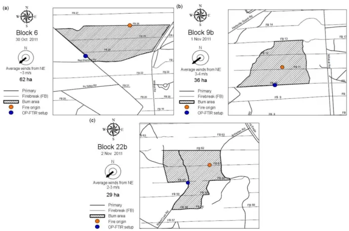
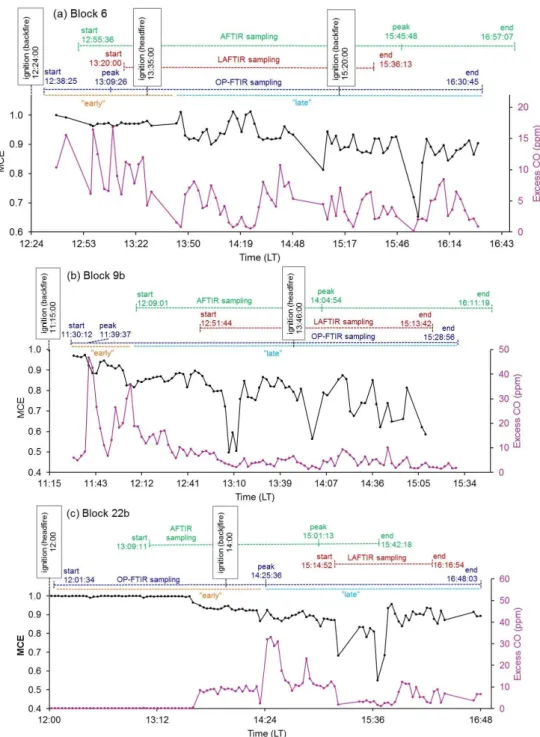
Unlike the LAFTIR and AFTIR, the OP-FTIR was set up be-fore the burns on a pre-selected portion of the fire perime-ter. For each fire the OP-FTIR was positioned to capture the downwind smoke emitted shortly after the fire ignition commenced. Figure 2 shows the burn blocks at Fort Jack-son and the relative placement of the OP-FTIR for each fire. After ignition, the OP-FTIR sampled a variety of emissions as detailed next. Figure 3 shows the OP-FTIR time series of MCE and excess CO (ppm) that can be used as indicators of the combustion type and intensity the OP-FTIR observed on each fire. The AFTIR and LAFTIR sampling time periods and fire ignition times are also shown.
During the Block 6 fire, light and variable winds were from the northeast and the OP-FTIR was positioned along the southwest perimeter of the fire area with an optical path of 32.2 m (Fig. 2a). A backing fire was started at 12:24 local time (LT, EDT) on the southwestern perimeter of the burn block along the same firebreak as the OP-FTIR setup. The heading fire was initiated at the opposite end of the block at 13:35 LT, with more backfires lit to increase the fire inten-sity at∼15:20 LT. The most intense column of smoke of the
day was sampled by AFTIR∼25 min later around 15:46 LT
(Fig. 3a).
Fig. 2.Detailed burn maps of(a)Block 6,(b)Block 9b, and(c)Block 22b prescribed fires at Fort Jackson, SC. The location of the OP-FTIR is shown as a blue circle. The location where the fire was first lit is shown by the orange circle. Fires were typically lit along firebreaks in a continuous line with the “fire origin” representing where the fire-line was initiated.
∼25 min later and the AFTIR peaked ∼35 min after that
(Fig. 3c).
3.1.2 AFTIR
The AFTIR airborne sampling strategy is detailed in Akagi et al. (2013). To measure the initial emissions, lofted smoke less than several minutes old was sampled by penetrating the smoke column 150 to several thousand meters from the flame front (Fig. 1c). The smoke sampled by the AFTIR was pro-duced by flaming combustion of understory and canopy fu-els with a significant contribution (∼40 %, Yokelson et al., 1996) from smoldering emissions that became entrained in the single, main updraft core. AFTIR sampling periods and peak smoke samples are seen in Fig. 3.
3.1.3 LAFTIR
The LAFTIR ground-based sampling protocol was similar to that described in Burling et al. (2011) and Akagi et al. (2013). Backgrounds were acquired before the fire. Ground-based sampling access was sometimes precluded during ignition, but sampling access then continued through late afternoon until the fire was effectively out. During post-ignition access, numerous point sources of RSC were sought out and
sam-pled with the LAFTIR system minutes to hours after passage of a flame front. Spot sources of white smoke, mainly pro-duced from pure smoldering combustion, included smolder-ing stumps, fallen logs, litter layers, etc., and they contributed to a dense smoke layer below the canopy. The LAFTIR sometimes sampled in the vicinity of the OP-FTIR, but fre-quently roved to other areas. The LAFTIR sampling period for each fire is shown in Fig. 3.
3.2 MCE, initial emissions, and a comparison
of flaming- and smoldering-dominated combustion measured by OP-FTIR
3.2.1 MCE and initial emissions
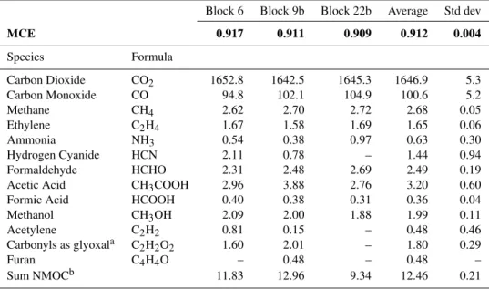
OP-FTIR fire-average MCEs and EFs are shown in Table 1. The OP-FTIR MCEs across all fires showed minimal vari-ability with a study-average of 0.912±0.004 compared to the LAFTIR (0.842±0.046) and AFTIR (0.929±0.008).
The average MCE for full fires burning SE US DoD fuels in the lab was 0.937±0.024 (Burling et al., 2010). The
Fig. 3.MCE (black) and excess CO (ppm, pink) time series from OP-FTIR on the three Fort Jackson fires. Above the time series, AFTIR (green), LAFTIR (red), and OP-FTIR (dark blue) sampling time frames are shown to denote the start and end of measurement collection and when the “peak” intensity signal was observed from a given measurement platform. “Early” and “late” periods of OP-FTIR sampling are denoted in orange and light blue, respectively. Ignition times are shown in black to mark the lighting of headfires and backfires.
(less than 18.6 % fire-average relative standard deviation, or RSD). The major exceptions were acetylene (96.4 % RSD) and the two nitrogen-containing compounds, HCN (65.3 % RSD) and NH3(48.6 % RSD). The high variability in the
lat-ter two compounds is not surprising since the highly variable nitrogen content of biomass fuel can have a large influence on the emissions of N-containing species (Burling et al., 2011).
High variability in acetylene has been observed in the lit-erature and is likely attributed to the fact that C2H2 can be
Table 1.MCE (bolded) and EFs (g kg−1)for three pine understory burns measured by OP-FTIR.
Block 6 Block 9b Block 22b Average Std dev
MCE 0.917 0.911 0.909 0.912 0.004
Species Formula
Carbon Dioxide CO2 1652.8 1642.5 1645.3 1646.9 5.3
Carbon Monoxide CO 94.8 102.1 104.9 100.6 5.2
Methane CH4 2.62 2.70 2.72 2.68 0.05
Ethylene C2H4 1.67 1.58 1.69 1.65 0.06
Ammonia NH3 0.54 0.38 0.97 0.63 0.30
Hydrogen Cyanide HCN 2.11 0.78 – 1.44 0.94
Formaldehyde HCHO 2.31 2.48 2.69 2.49 0.19
Acetic Acid CH3COOH 2.96 3.88 2.76 3.20 0.60
Formic Acid HCOOH 0.40 0.38 0.31 0.36 0.04
Methanol CH3OH 2.09 2.00 1.88 1.99 0.11
Acetylene C2H2 0.81 0.15 – 0.48 0.46
Carbonyls as glyoxala C2H2O2 1.60 2.01 – 1.80 0.29
Furan C4H4O – 0.48 – 0.48 –
Sum NMOCb 11.83 12.96 9.34 12.46 0.21
aThe residual spectrum from 2820 to 2850 cm−1(after fitting HCHO, CH
4, and H2O) contained features similar to glyoxal, but
shifted by several wavenumbers. The feature may have been due to a mixture of oxygenated compounds (most likely carbonyls), but was analyzed using the glyoxal IR cross-section (Profeta et al., 2011).bNon-methane organic compounds.
3.2.2 Comparison of flaming- and
smoldering-dominated combustion sampled by OP-FTIR
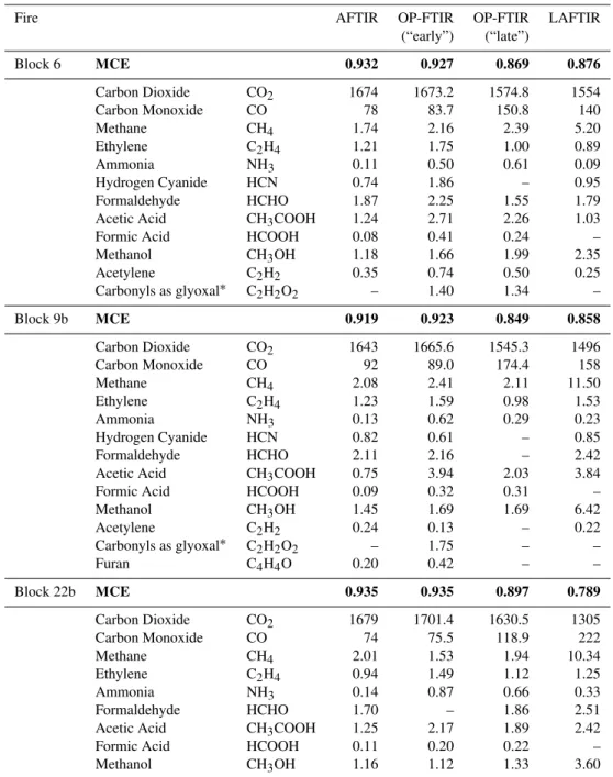
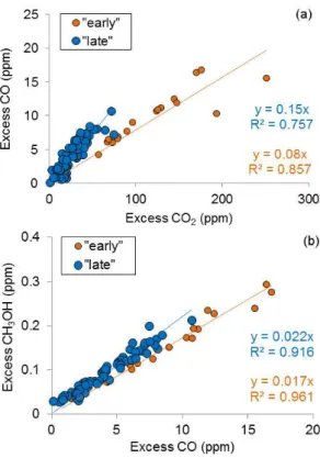
Fire-average EFs are important when assessing overall fire characteristics or when comparing to other fire-average EF in the literature. That being said, the drop in OP-FTIR MCE seen partway through each Fort Jackson fire (Fig. 3) suggests that EF computed separately for “early” and “late” time blocks would be mainly indicative of flaming- and smoldering-dominated combustion, respectively. In fact, the calculation of OP-FTIR EF for “early” and “late” periods did inform the comparison to EF measured from other plat-forms. It should be noted that not all fire measurements show a fast transition between high and low MCE (Yokelson et al., 1996) and the division between “early” and “late” can be indistinct. However, this informal separation is one use-ful way to probe the dynamic mix of flaming and smolder-ing combustion and compare to other platforms. Delineation between “early” and “late” are seen for the three fires in Fig. 3. As an example, on the Block 6 fire, “early” was de-fined from the first OP-FTIR sample (12:38:25 LT) until a no-ticeable drop in MCE is observed (13:47:00 LT, upper trace, black, Fig. 3a). This signifies a change in the composition of the sampled smoke from mostly flaming to more smoldering combustion. Emission factors for “early” and “late” smoke measured by OP-FTIR from the Fort Jackson fires are shown in Table 2. This shift from flaming- to smoldering-dominated combustion is also noted in the ER plots for several species, including CO and methanol (Fig. 4). Both species are pri-marily produced from smoldering combustion and thus, a
higher ratio of1CO /1CO2and1CH3OH /1CO was
ob-served when sampling “late” smoke that had a greater con-tribution from un-lofted RSC (“late” data are shown in blue). CO had a large EF range, with EF(CO) “late” being almost twice as large as EF(CO) “early”. While we generally ob-serve higher OP-FTIR EF for some smoldering compounds late in the fire associated with lower MCE, we note that this trend was not consistently observed across all fires and plat-forms. Additionally, we observe mixed, somewhat anoma-lous results likely rooted in fuel differences for other species such as ammonia, ethylene, acetic acid, formaldehyde, and formic acid (Table 2). On the Block 9b fire, the EF for NH3
and CH3COOH are twice as large for the early flaming
dom-inated OP-FTIR samples as they are for the later smoldering dominated samples, despite the fact that these compounds are well-known to be associated with smoldering emissions. It is possible that the OP-FTIR may be relatively more influenced by recirculated emissions from burning live fuels early in the fire.
3.3 OP-FTIR data compared with LAFTIR and AFTIR
FTIR platforms
It is of interest to compare the emission factors from all three FTIRs employed during the Fort Jackson burns since each FTIR had a different spatial and temporal perspec-tive on the overall combustion emissions. Figure 5 shows a side-by-side comparison of OP-FTIR, LAFTIR, and AF-TIR fire-averaged emission factors from all three Fort Jack-son fires. The study-average MCEs were 0.929±0.008,
Table 2.MCE (bolded) and EFs (g kg−1)for select compounds measured during “early” and “late” blocks by OP-FTIR. Fire-averaged EF from the AFTIR and LAFTIR (Akagi et al., 2013) are also shown.
Fire AFTIR OP-FTIR OP-FTIR LAFTIR
(“early”) (“late”)
Block 6 MCE 0.932 0.927 0.869 0.876
Carbon Dioxide CO2 1674 1673.2 1574.8 1554
Carbon Monoxide CO 78 83.7 150.8 140
Methane CH4 1.74 2.16 2.39 5.20
Ethylene C2H4 1.21 1.75 1.00 0.89
Ammonia NH3 0.11 0.50 0.61 0.09
Hydrogen Cyanide HCN 0.74 1.86 – 0.95
Formaldehyde HCHO 1.87 2.25 1.55 1.79
Acetic Acid CH3COOH 1.24 2.71 2.26 1.03
Formic Acid HCOOH 0.08 0.41 0.24 –
Methanol CH3OH 1.18 1.66 1.99 2.35
Acetylene C2H2 0.35 0.74 0.50 0.25
Carbonyls as glyoxal∗ C2H2O2 – 1.40 1.34 –
Block 9b MCE 0.919 0.923 0.849 0.858
Carbon Dioxide CO2 1643 1665.6 1545.3 1496
Carbon Monoxide CO 92 89.0 174.4 158
Methane CH4 2.08 2.41 2.11 11.50
Ethylene C2H4 1.23 1.59 0.98 1.53
Ammonia NH3 0.13 0.62 0.29 0.23
Hydrogen Cyanide HCN 0.82 0.61 – 0.85
Formaldehyde HCHO 2.11 2.16 – 2.42
Acetic Acid CH3COOH 0.75 3.94 2.03 3.84
Formic Acid HCOOH 0.09 0.32 0.31 –
Methanol CH3OH 1.45 1.69 1.69 6.42
Acetylene C2H2 0.24 0.13 – 0.22
Carbonyls as glyoxal∗ C2H2O2 – 1.75 – –
Furan C4H4O 0.20 0.42 – –
Block 22b MCE 0.935 0.935 0.897 0.789
Carbon Dioxide CO2 1679 1701.4 1630.5 1305
Carbon Monoxide CO 74 75.5 118.9 222
Methane CH4 2.01 1.53 1.94 10.34
Ethylene C2H4 0.94 1.49 1.12 1.25
Ammonia NH3 0.14 0.87 0.66 0.33
Formaldehyde HCHO 1.70 – 1.86 2.51
Acetic Acid CH3COOH 1.25 2.17 1.89 2.42
Formic Acid HCOOH 0.11 0.20 0.22 –
Methanol CH3OH 1.16 1.12 1.33 3.60
∗The residual spectrum from 2820 to 2850 cm−1(after fitting HCHO, CH
4, and H2O) contained features similar to glyoxal, but
shifted by several wavenumbers. The feature may have been due to a mixture of oxygenated compounds (most likely carbonyls), but was analyzed using the glyoxal IR cross-section (Profeta et al., 2011).
and LAFTIR platforms, respectively (calculated from Ta-ble 2). The MCEs from the AFTIR and LAFTIR indicate larger contributions from flaming and smoldering combus-tion, respectively. We observe a general trend for some smol-dering species whose emissions depend more strongly on MCE than fuel type (e.g. CH4, CH3OH, furan) – namely:
EF(AFTIR) < EF(OP-FTIR) < EF(LAFTIR), which is con-sistent with the decreasing trend in FTIR fire-averaged
MCEs. However, exceptions exist when considering all fires and all platforms. For nitrogen compounds whose emis-sions are typically more fuel dependent (e.g. HCN, NH3),
a general EF(AFTIR < EF(LAFTIR) < EF(OP-FTIR) trend was observed.
flaming-/smoldering-Fig. 4.ER plots of(a)1CO /1CO2and(b)1CH3OH /1CO from the Block 6 (30 October) fire with two trend-lines shown: samples collected “early” in the fire are shown as orange circles and those collected “late” in the fire are shown as blue circles. Different trends observed “early” and “late” in the fire’s progression imply changes in the sampled smoke over time and a decrease in MCE.
dominated phases to further investigate general trends ob-served in Fig. 5. Table 2 includes a detailed comparison of emissions from different platforms and different fires, with OP-FTIR EF divided into “early” and “late” sampling peri-ods. These data are visually represented in Fig. 6. The OP-FTIR (“early”) MCE is similar to the AOP-FTIR MCE on all fires. This is expected, since the smoke observed by the OP-FTIR during the initial phase of the fire was mostly flaming emissions. Alternately, the OP-FTIR (“late”) MCE is simi-lar to the LAFTIR MCE on the Block 6 and Block 9b fires, which is also expected since the OP-FTIR (“late”) phase sampled mostly smoldering debris after passage of the flame front. However, beyond these similarities no consistent trend is seen. For instance, the values for LAFTIR CH4 are 2–5
times higher than the values for OP-FTIR “late” at similar MCE. The data are highly variable and the passively-sampled OP-FTIR values may be less biased than the LAFTIR val-ues. Some of the EF that were higher for OP-FTIR compared to the other two platforms are also known as “sticky” com-pounds that can be difficult to sample in closed-cell systems (NH3 and HCOOH). However, small to no losses of these
species were observed during 120–180 s storage in the closed cells and the residence times in the coated/Teflon inlets are
only 1–2 s. Further, losses on the cell walls were measured and corrected for in both closed cell FTIR systems accord-ing to a protocol developed by Yokelson et al. (2003) who directly compared AFTIR and OP-FTIR systems in the same well-mixed laboratory smoke samples. If the passivation cor-rections were accurate, then the higher study-average EF by OP-FTIR for some species in this work may largely be due to sampling emissions from a different mix of fuels. This idea is supported by the fact that EFs for HCN, HCHO, and C2H4,
which are generally smoldering compounds that do not suffer from wall losses, are also higher in OP-FTIR than the closed cell systems. In addition, the NH3 EFs agree well for the
LAFTIR and OP-FTIR “late” period on one fire (Block 9b). Nevertheless, we acknowledge that open-path measurements are inherently immune to sampling losses for such species and if the closed cell correction factors are too small, then fires may emit more NH3 or HCOOH than our previous
closed-cell measurements indicate (Akagi et al., 2011). Re-gardless of the reason for the study-average differences be-tween the FTIRs (e.g. fuel differences, temperature differ-ences (Aan de Brugh et al., 2012), sampling issues (Norman et al., 2009)), the EFs from the OP-FTIR show that flaming influenced the ground level smoke layer.
3.4 OP-FTIR comparisons with the literature
We can compare the OP-FTIR EF with those from a study that employed a similar open-path FTIR to mea-sure biomass burning emissions from South African sa-vanna fires (Wooster et al., 2011). The fire-averaged MCE and1CO /1CO2, respectively, from Wooster et al. (2011)
(0.913±0.026 and 0.095) are similar to those in this work (0.912±0.004 and 0.095). This similarity in fire-average MCE and 1CO /1CO2 is surprising considering
pine-understory and savanna fuels are intrinsically different and have been measured from airborne platforms at different MCE and1CO /1CO2(pine-understory: 0.931±0.016 and
0.074; savanna: 0.944±0.012 and 0.059; Akagi et al., 2011,
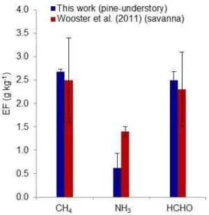
2013). Savannas are usually dominated by fine fuels that burn at high combustion efficiency (Akagi et al., 2011) and do not often include large diameter fuels highly susceptible to pro-longed smoldering. Temperate pine understory ecosystems often have more dead/down debris and below-ground fuels like organic soils that tend to burn by smoldering and/or RSC although that is minimized in prescribed fires. The Wooster et al. (2011) fires were not sampled by an airborne platform, thus, we cannot compare both OP-FTIR and AFTIR MCEs between the studies. We can compare emissions for several species from this work and Wooster et al. (2011) (Fig. 7). Emission factors from this work are all within the natural variability of EF (computed as the 1-σ standard deviation of fire-averaged EF reported by Wooster et al., 2011), except for NH3. As mentioned in Sect. 3.2.1, multiple factors can
Fig. 5.Side-by-side comparison of study-average emission factors between the AFTIR (green), OP-FTIR (blue), and LAFTIR (red) FTIRs
employed during the Fort Jackson campaign. The EFs and error bars represent the average EF and 1-σ standard deviation over all three of
the Fort Jackson fires, respectively.
et al. (2011) were acquired at Kruger National Park where elephant dung is a major fuel component. Dung is known to have a higher nitrogen content compared with other biomass types (Christian et al., 2007; Keene et al. 2006). While the N content of fuels sampled in this work and in Wooster et al (2011) is unknown, higher fuel N could explain why EF(NH3)was significantly higher in Wooster et al. (2011). 3.5 Estimating fire-line exposure to air toxics
Smoke has numerous and varied possible health effects, es-pecially for fire-line workers who are subjected to it on a routine basis. Quantification, of ground-level concentrations over the duration of a prescribed fire is one part of assess-ing the risk. The measured exposures can then be com-pared to laws and guidelines that estimate potentially harm-ful levels of toxins. Average concentrations over time and peak exposures are both of concern: in the US, the Occu-pational Safety and Health Administration (OSHA) sets le-gal exposure limits known as permissible exposure limits (PELs) and short-term exposure limits (STELs) for these two cases, respectively. A PEL is a time-weighted average (TWA) concentration not to be exceeded for routine 8 h exposure while a STEL should not be exceeded for any 15–30 min period. The National Institute of Occupational Safety and Health (NIOSH) provide Recommended Exposure Limits, or RELs, as TWA concentrations for an 8 h or 10 h workday. NIOSH also reports STELs as a 15 min maximum exposure. NIOSH limits, being guidelines, are often more conservative than those enforced by OSHA (Sharkey, 1997). In addition to NIOSH, the American Conference of Industrial Hygienists (ACGIH) sets exposure guidelines known as Threshold Limit Values (TLVs). The ACGIH TLV is an 8 h TWA and the TLV STEL is a 15 min maximum exposure. In our analysis we re-port a range when more than one exposure limit/guideline is available.
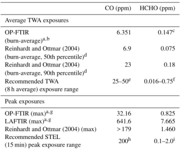
Table 3 shows measured TWA burn-average and peak ex-posures for CO and HCHO from this work, other works (Reinhardt and Ottmar, 2004), and the recommended TWA (8 h) and STEL exposure ranges. We first compare OP-FTIR burn-average TWA concentrations to those from Reinhardt and Ottmar (2004), who report a frequency distribution of line exposures as a cumulative percent of sampled fire-fighters measured from prescribed burns in the Northwest. The CO burn-average mixing ratio exposure for firefight-ers in the 50th percentile from Reinhardt and Ottmar (2004) was slightly higher (by 8.6 %) than the burn-average con-centration measured in this work, while their HCHO 50th percentile concentration was approximately a factor of two lower than in our work. Location, fuel, weather, and fuel moisture are just some of the variables that could have created very different burn conditions between our study and that of Reinhardt and Ottmar (2004). OP-FTIR burn-averaged exposures can also be compared with recom-mended TWA exposures. Our burn-average 1CO was be-low all the recommended exposure levels while our burn-average1HCHO was near the lower end of exposure guide-lines (0.016–0.75 ppm range). Thus, Fort Jackson1CO and 1HCHO did not exceed OSHA guidelines suggesting that prolonged exposures were a limited problem for these com-pounds during the Fort Jackson fires.
3
2
1
0
Emission Factor (g kg
-1 ) 6
3
AFTIR OP-FTIR (early) OP-FTIR (late) LAFTIR
Block 6 (a)
5
4
3
2
1
0
Emission Factor (g kg
-1 )10
5 Block 9b
(b)
4
3
2
1
0
Emission Factor (g kg
-1) 128
4 Block 22b
(c)
CH4 C2H4 HCHO CH3COOH HCOOH CH3OH C2H2 Carbonyls
as glyoxal C4H4O NH3 HCN
Fig. 6.Emission factors (g kg−1)measured by the AFTIR (green), OP-FTIR, and LAFTIR (red) from the three Fort Jackson fires:(a)
Block 6,(b)Block 9b, and(c)Block 22b. The OP-FTIR EF have been broken down into “early” (orange) and “late” (blue) as shown in
Fig. 3. Error bars represent the relative uncertainty in the EF. A break has been added in the uppermostyaxis EF values that applies only to
CH4and CH3OH, when applicable.
Fig. 7.Comparison of emission factors from this work (blue) and Wooster et al. (2011) (red). EF from this work have been slightly recalculated using a similar mass balance of carbon as dictated by measured species from Wooster et al. (2011), and are thus slightly different than EF shown in Table 1.
LAFTIR values represent a mostly avoidable upper limit, as these mixing ratios were measured by placing the sample line less than 1 m from smoldering point sources.
Thus far we have limited our discussion of air toxins to CO and HCHO, though many others exist. Exposure to the other air toxins not measured by the OP-FTIR can be estimated using normalized excess mixing ratios (1X /1CO where
“X” is an air toxin) measured in other studies and multiply-ing by the OP-FTIR burn-average CO. Exposure estimates have previously been derived this way by Austin (2008) who used published EFs and ceiling limits to calculate “hazard ra-tios”. We use a slightly different approach: we estimate TWA and peak exposures of high risk compounds using a recent comprehensive set of pine-understory prescribed fire emis-sion ratios from Yokelson et al. (2013) and multiply those ER by the OP-FTIR burn-average and peak1CO. For air toxins measured both by OP-FTIR and Yokelson et al. (2013) we can “test” this approach by comparing “estimated” vs. “mea-sured” exposures (for HCHO, CH3OH, NH3, see Table A2
in Appendix A). In most cases the estimated mixing ratios are lower than the measured mixing ratios by up to 65 %, ex-cept for HCHO and NH3measured by the LAFTIR; e.g., the
greatest deviation from 1 was the estimated/measured value of 6.60 for the NH3 LAFTIR peak exposure. Given such a
high ratio (based on comparison to AFTIR measurements from 2010) it is clear that this estimation technique is less ap-plicable for N-containing compounds since their emissions depend strongly on fuel N (Burling et al., 2011). It is also important to note that the emissions data from Yokelson et al. (2013) are mostly for the 2010 pine understory prescribed fires at Camp Lejeune that were lit after a wet spring ver-sus older growth stands lit after a prolonged drought in this work. Excluding the one anomalously high NH3ratio
men-tioned above, the average estimated/measured ratio and 1-σ standard deviation is 0.69±0.38. Thus, smoke is variable,
Table 3.Average TWA and peak exposures measured in this work and other studies and recommended TWA and peak exposures.
CO (ppm) HCHO (ppm)
Average TWA exposures
OP-FTIR 6.351 0.147c
(burn-average)a,b
Reinhardt and Ottmar (2004) 6.9 0.075 (burn-average, 50th percentile)d
Reinhardt and Ottmar (2004) 23 0.18 (burn-average, 90th percentile)d
Recommended TWA 25–50e 0.016–0.75f (8 h average) exposure range
Peak exposures
OP-FTIR (max)a,g 32.16 0.825 LAFTIR (max)a,g 641.6 7.665 Reinhardt and Ottmar (2004) (max) > 179 1.460 Recommended STEL
200h 0.1–2.0i (15 min) peak exposure range
aReported as excess mixing ratios. Absolute values will be slightly higher to account
for background concentrations.bThe time at the prescribed burns averaged 4:13 h (range
∼4–5 h).cSince we do not report HCHO measured from the start to end of the Fort Jackson fires, this value was estimated as ER(HCHO / CO)×OP-FTIR (burn-average)
1CO.dThe time at the prescribed burns averaged 7 h (range 2–13 h).eLow and high
CO values represent ACGIH TWA TLV and OSHA TWA PEL, respectively.fLow and high HCHO values represent NIOSH TWA REL and OSHA TWA PEL, respectively.
gPeak exposures represent the average maximum peak exposure from the three
different fires measured.hNIOSH ceiling and OSHA STEL (5 min).iLow and high values represent NIOSH STEL and OSHA STEL, respectively.
Based on this methodology we present estimated expo-sures to many air toxins not measured in this work, but reported in Yokelson et al. (2013) (Table 4). All of the species listed in Table 4 are designated as hazardous air pol-lutants, or harmful or potentially harmful constituents in to-bacco smoke as noted by Yokelson et al. (2013). Our esti-mated fire-line TWA exposures based on OP-FTIR burn av-erage CO are significantly lower than recommended TWA exposure limits (a factor of 10 lower at the least), suggest-ing that reasonably cautious personnel on the Fort Jackson fires likely did not exceed individual recommended expo-sure limits for the hazardous compounds listed in Table 4. Even estimated peak exposures based on LAFTIR peak CO were lower than recommended STELs except for acrolein and HCN, which exceeded STELs by factors of 3.7 and 1.2, respectively. We also show estimated exposures divided by the recommended TWA exposure limits, orEx, where
X is a given compound of interest.Excan be used to
cal-culate a unitless irritant exposure mixture termEm, where
Em=Ex1+Ex2+Ex3+. . . (Reinhardt and Ottmar, 2004). For
example,Exfor compounds such as acrolein and
formalde-hyde can be summed and ifEmexceeds 1, then the
combi-nation of the irritants exceeds the combined exposure limit (Sharkey, 1997). Only considering acrolein (Table 4) and formaldehyde (Table 3), we report a TWA combined irritant exposureEm of 0.31 which is not in exceedance of OSHA
limits but only lower by a factor of∼3, showing that com-bined TWA exposures are a greater concern than TWA posures assessed individually. However, we note that the ex-posure mixture equation is a simplification of complex phe-nomena and it is unlikely that the effects of toxins add lin-early (Yokelson et al., 2013; Menser and Heggestad, 1966; Mauderly and Samet, 2009). Em is used as an estimate of
combined exposure effects as the actual synergistic effects of a given pollutant combination are unknown. Additionally, we ignore the effects of particles which likely affect expo-sure limits for individual and combined species (Pope and Dockery, 2006; Adetona et al., 2011). This work agrees with previous works that “shift-average” TWA exposures may be less of a problem than peak exposures (Sharkey, 1997; Rein-hardt and Ottmar, 2004; Austin, 2008), however, combined TWA exposures must be considered for a more realistic as-sessment of fire-line risk.
4 Conclusions
We measured trace gas emission factors for three prescribed fires at Fort Jackson, SC using an open-path Fourier trans-form infrared (OP-FTIR) system. The fires occurred outside the common range of conditions for southeastern US pre-scribed fires because the fuels included stands that had not been burned by prescribed fire in decades and the stands had recently been subject to drought. Thus, the emissions may be somewhat relevant to a scenario where frequency of pre-scribed fire is reduced, or to a wildfire.
The OP-FTIR measured a fire-averaged modified combus-tion efficiency (MCE) closer to that of the airborne FTIR (AFTIR) system than to the land-based FTIR (LAFTIR). This suggests that local ignition before plume development and to a lesser extent, downdrafts after plume development, may contribute significantly to the ground level smoke layer. Burn managers maximize smoke lofting so airborne mea-surements provide the best fire integrated sample in the ab-sence of abundant residual smoldering combustion (RSC). However, the LAFTIR enables modeling of specific RSC fu-els, but the OP-FTIR may be a less biased sample of the ground-level smoke layer. More coordinated and extensive ground-based sampling of emissions and fuel consumption would be of value in future experiments.
Table 4.Estimated OP-FTIR TWA burn-averaged and peak concentrations, LAFTIR peak concentrations, and recommended TWA and peak exposures.
Estimated OP Recommended Ex(estimated Estimated OP- Estimated Recommended
-FTIR TWA TWA exposure exposure/ FTIR peak LAFTIR peak STEL peak exposure (ppm)a (ppm)b Recommended exposure exposure exposure exposure)c (ppm)a (ppm)a (ppm)d Acrolein (C3H4O) 0.0109 0.1 1.09×10⁻¹ 0.055 1.102e 0.3
Ammonia (NH3)f 0.206 25–50 4.12×10⁻³ 0.493 1.106 35
Benzene (C6H6) 0.0058 0.1–1.0 5.81×10⁻³ 0.029 0.587 1.0–5.0
Hydrogen Cyanide (HCN) 0.0540 10 5.40×10⁻³ 0.273 5.456e 4.5 Hydrochloric Acid (HCl) 0.0043 2.0–5.0 8.68×10⁻⁴ 0.022 0.438 3.0–7.0 Acetonitrile (CH3CN) 0.0079 20–40 1.98×10⁻⁴ 0.040 0.801 60
Acetaldehyde (CH3CHO) 0.0385 100 3.85×10⁻⁴ 0.195 3.885 150
Formaldehyde (HCHO)f 0.147 0.016–0.75 1.96×10⁻¹ 0.825 7.665 0.1–2.0
Methanol (CH3OH)f 0.1200 200 6.00×10⁻⁴ 0.560 15.65 250
Acrylonitrile (C3H3N) 0.0010 1.0–2.0 5.07×10⁻⁴ 0.005 0.102 10
1,3-Butadiene (C4H6) 0.0001 1.0–2.0 7.48×10⁻⁵ 0.0004 0.008 5
Propanal (C3H6O) 0.0043 20 2.14×10⁻⁴ 0.022 0.433 –
Acetone (C3H6O) 0.0150 250–1000 1.50×10⁻⁵ 0.076 1.514 1000
1,1-Dimethylhydrazine (C2H8N2) 0.0014 0.5 2.70×10⁻³ 0.007 0.136 –
Crotonaldehyde (C4H6O) 0.0074 2.0 3.68×10⁻³ 0.037 0.743 –
Acrylic Acid (C3H4O2) 0.0013 2.0–10.0 1.33×10⁻⁴ 0.007 0.134 –
Methyl Ethyl Ketone (MEK, C4H8O) 0.0041 200 2.07×10⁻⁵ 0.021 0.418 300
n-Hexane (C6H14) 0.0006 50–500 1.21×10⁻⁶ 0.003 0.061 510
Toluene (C6H5CH3) 0.0038 50–200 1.89×10⁻⁵ 0.019 0.381 500
Phenol (C6H5OH) 0.0088 5 1.76×10⁻³ 0.044 0.887 15.6
Methyl Methacrylate (C5H8O2) 0.0009 50–100 9.21×10⁻⁶ 0.005 0.093 100
Styrene (C8H8) 0.0012 20–100 1.16×10⁻⁵ 0.006 0.117 40–200
Xylenes (C8H10) 0.0031 100 3.07×10⁻⁵ 0.016 0.310 150–200
Ethylbenzene (C8H10) 0.0009 100 8.95×10⁻⁶ 0.005 0.090 125
Naphthalene (C10H8) 0.0038 10 3.83×10⁻⁴ 0.019 0.387 15
Isocyanic Acid (HNCO)g 0.0052 – – 0.026 0.524 –
aEstimated values reported as excess mixing ratios. Absolute values will be slightly higher to account for background concentrations.bReported as OSHA TWA PEL, NIOSH TWA REL, and/or
ACGIH TWA TLV.cEstimated exposures (ppm) were divided by the recommended OSHA TWA exposures (ppm) to aid in the estimation of combined exposure limits. When OSHA TWA were not available, ACGIH TWA TLV were used.dReported as OSHA STEL, NIOSH STEL, and/or ACGIH TLV STEL.eExceeds recommended STEL peak exposure limit.fMeasured values from Table 3 are shown instead of estimated values.gRoberts et al. (2011) suggest mixing ratios above 0.001 ppm may have physiological effects, but no recommendations have been established.
environment coupled with the spatial separation between the systems. The largest differences between ground-based sys-tems were seen for CH4(factor of five) and the largest
dif-ferences between AFTIR and OP-FTIR were for NH3, which
was higher by ground-based OP-FTIR than from an aircraft. The chemistry and amount of un-lofted emissions is not highly constrained suggesting that some fires may produce higher overall NH3emissions than would be implied by
air-borne measurements (Griffith, 1991; Wooster et al., 2011). We also observed very similar EF between this work and EF measured on prescribed African savanna fires by a sim-ilar OP-FTIR system, despite the fact that the fires burned in very different ecosystems, fuel types, weather conditions, etc. This also suggests that MCE and trace gas EFs can be highly dependent on the measurement platform.
Average and peak OP-FTIR mixing ratios and peak LAFTIR mixing ratios were compared to recommended time-weighted average (TWA) and peak exposure guidelines. We also estimated TWA and peak exposures for many air tox-ins not measured in this work by ratioing normalized excess
mixing ratios from a comprehensive study to our real fire-line CO data. This is an important approach to estimating ex-posures since it would be difficult to deploy large amounts of advanced instrumentation on a fire-line. Our data sup-port previous findings that peak exposures are more likely to challenge permissible exposure limits than average expo-sures, suggesting it is important for wildland fire personnel to avoid concentrated smoldering smoke to minimize their risk of overexposure.
Appendix A
Table A1.Spectral regions used to retrieve excess mixing ratios reported in this work.
Target Spectral region Other species Single Beam (SB) or
species (cm−1) fitted Transmission (T)
CO, CO2 2050–2330 H2O SB
CH4 2990–3105 H2O SB
C2H4, NH3 922–975 H2O TR
CH3OH 1020–1055 NH3, H2O TR
CH3COOH, HCOOH 1100–1230 H2O, CH4, NH3 TR
HCN 709–717 H2O TR
C2H2, Furan 725–755 H2O, CO2, 2-Methylfuran TR
HCHO, Glyoxal 2740–2850 CH4, H2O TR
Table A2.Estimated and measured exposures for species measured both by the OP-FTIR and in Yokelson et al. (2013) reported as excess mixing ratios (see Sect. 3.5 for discussion).
OP-FTIR TWA OP-FTIR peak LAFTIR peak
exposure (ppm) exposure (ppm) exposure (ppm)
Formaldehyde (HCHO) Estimateda 0.12 0.63 12.52
Measuredb 0.147c 0.825 7.665
Estimated/Measured 0.82 0.76 1.63
Methanol (CH3OH) Estimateda 0.081 0.409 8.165
Measured 0.120 0.56 15.65
Estimated/Measured 0.67 0.73 0.52
Ammonia (NH3) Estimateda 0.072 0.366 7.304
Measured 0.206 0.493 1.106
Estimated/Measured 0.35 0.74 6.60
aEstimated from pine-understory fire ER(1X /1CO) (from Yokelson et al., 2013) multiplied by the burn-average1CO measured by the
OP-FTIR (Table 3).bShown in Table 3.cSince we do not report HCHO measured from the start to end of the Fort Jackson fires, this value was estimated as ER(1HCHO /1CO)×OP-FTIR (burn-average)1CO.
Acknowledgements. This work was supported by the Strategic Environmental Research and Development Program (SERDP) project RC-1649 and administered partly through Forest Service Research Joint Venture Agreement 08JV11272166039, and we thank the sponsors for their support. We greatly appreciate the collaboration and efforts of John Maitland and forestry staff at Fort Jackson.
Edited by: P. O. Wennberg
References
Aan de Brugh, J. M. J., Henzing, J. S., Schaap, M., Morgan, W. T., van Heerwaarden, C. C., Weijers, E. P., Coe, H., and Krol, M. C.: Modelling the partitioning of ammonium nitrate in the convective boundary layer, Atmos. Chem. Phys., 12, 3005–3023, doi:10.5194/acp-12-3005-2012, 2012.
Achtemeier, G. L.: Measurements of moisture in smoldering smoke and implications for fog, Int. J. Wildland Fire, 15, 517–525, doi:10.1071/WF05115, 2006.
Adetona, O., Dunn, K., Hall, D. B., Achtemeier, G., Stock, A., and
Naeher, L. P.: Personal PM2.5 exposure among wildland
fire-fighters working at prescribed forest burns in southeastern United States, J. Occup. Environ. Hyg., 8, 503–511, 2011.
Akagi, S. K., Yokelson, R. J., Wiedinmyer, C., Alvarado, M. J., Reid, J. S., Karl, T., Crounse, J. D., and Wennberg, P. O.: Emis-sion factors for open and domestic biomass burning for use in atmospheric models, Atmos. Chem. Phys., 11, 4039–4072, doi:10.5194/acp-11-4039-2011, 2011.
Akagi, S. K., Craven, J. S., Taylor, J. W., McMeeking, G. R., Yokel-son, R. J., Burling, I. R., Urbanski, S. P., Wold, C. E., Seinfeld, J. H., Coe, H., Alvarado, M. J., and Weise, D. R.: Evolution of trace gases and particles emitted by a chaparral fire in California, Atmos. Chem. Phys., 12, 1397–1421, doi:10.5194/acp-12-1397-2012, 2012.
Akagi, S. K., Yokelson, R. J., Burling, I. R., Meinardi, S., Simp-son, I., Blake, D. R., McMeeking, G. R., Sullivan, A., Lee, T., Kreidenweis, S., Urbanski, S., Reardon, J., Griffith, D. W. T., Johnson, T. J., and Weise, D. R.: Measurements of reactive trace
gases and variable O3formation rates in some South Carolina
Austin, C.: Wildland firefighter health risks and respiratory protec-tion. Institut de recherche Robert Sauvé en santé et en sécurité du travail (IRSST), Report R-572, 2008.
Benscoter, B. W., Thompson, D. K., Waddington, J. M., Flannigan, M. D., Wotton, B. M., de Groot, W. J., and Turetsky, M. R.: In-teractive effects of vegetation, soil moisture and bulk density on depth of burning of thick organic soils, Int. J. Wildland Fire, 20, 418–429, 2011.
Bertschi, I. T., Yokelson, R. J., Ward, D. E., Babbitt, R. E., Su-sott, R. A., Goode, J. G., and Hao, W. M.: Trace gas and particle emissions from fires in large diameter and belowground biomass fuels, J. Geophys. Res., 108, 8472, doi:10.1029/2002JD002100, 2003.
Biswell, H. H.: Prescribed burning in California wildlands vegeta-tion management, Berkeley, CA: University of California Press; p. 255, 1989.
Burling, I. R., Yokelson, R. J., Griffith, D. W. T., Johnson, T. J., Veres, P., Roberts, J. M., Warneke, C., Urbanski, S. P., Rear-don, J., Weise, D. R., Hao, W. M., and de Gouw, J.: Labora-tory measurements of trace gas emissions from biomass burn-ing of fuel types from the southeastern and southwestern United States, Atmos. Chem. Phys., 10, 11115–11130, doi:10.5194/acp-10-11115-2010, 2010.
Burling, I. R., Yokelson, R. J., Akagi, S. K., Urbanski, S. P., Wold, C. E., Griffith, D. W. T., Johnson, T. J., Reardon, J., and Weise, D. R.: Airborne and ground-based measurements of the trace gases and particles emitted by prescribed fires in the United States, Atmos. Chem. Phys., 11, 12197–12216, doi:10.5194/acp-11-12197-2011, 2011.
Carter, M. C. and Foster, C. D.: Prescribed burning and productivity in southern pine forests: a review, Forest Ecol. Manag., 191, 93– 109, 2004.
Christian, T. J., Yokelson, R. J., Carvalho Jr., J. A., Griffith, D. W. T., Alvarado, E. C., Santos, J. C., Neto, T. G. S., Veras, C. A. G., and Hao, W. M.: The tropical forest and fire emissions exper-iment: Trace gases emitted by smoldering logs and dung from deforestation and pasture fires in Brazil, J. Geophys. Res., 112, D18308, doi:10.1029/2006JD008147, 2007.
Cochrane, M. A., Moran, C. J., Wimberly, M. C., Baer, A. D., Finney, M. A., Beckendorf, K. L., Eidenshink, J., and Zhu, Z.: Estimation of wildfire size and risk changes due to fuels treat-ments, Int. J. Wildland Fire, 21, 357–367, 2012.
Crutzen, P. J. and Andreae, M. O.: Biomass burning in the trop-ics: Impact on atmospheric chemistry and biogeochemical cy-cles, Science, 250, 1669–1678, 1990.
Demers, P. A., Checkoway, H., Vaughan, T. L., Weiss, N. S., Heyer, N. J., and Rosenstock, L.: Cancer incidence among firefighters in Seattle and Tacoma, Washington (United States), Cancer Cause. Control, 5, 129–135, 1994.
Gosz, J. R., Dahm, C. N., and Risser, P. G.: Long-path FTIR mea-surement of atmospheric trace gas concentrations, Ecology, 69, 1326–1330, 1988.
Greene, D. F., Macdonald, S. E., Hauessler, S., Domenicano, S., Noel, J., Jayen, K., Charron, I., Guathier, S., Hunt, S., Gielau, E. T., Bergeron, Y., and Swift, L.: The reduction of organic-layer depth by wildfire in the North American boreal forest and its effect on tree recruitment by seed, Can. J. Forest Res., 37, 1012– 1023, 2007.
Griffith, D. W. T., Mankin, W. G., Coffey, M. T., Ward, D. E., and Riebau, A.: FTIR remote sensing of biomass burning emissions
of CO2, CO, CH4, CH2O, NO, NO2, NH3, and N2O, in Global
Biomass Burning: Atmospheric, Climatic, and Biospheric Impli-cations, MIT Press, edited by: Levine, J., 230–240, 1991. Griffith, D. W. T., Deutscher, N. M., Caldow, C., Kettlewell, G.,
Riggenbach, M., and Hammer, S.: A Fourier transform infrared trace gas and isotope analyser for atmospheric applications, At-mos. Meas. Tech., 5, 2481–2498, doi:10.5194/amt-5-2481-2012, 2012.
Hardy, C. C., Ottmar, R. D., Peterson, J. L., Core, J. E., and Sea-mon, P.: Smoke management guide for prescribed and wildland fire; 2001 ed., PMS 420-2, National Wildfire Coordinating group, Boise, ID. 226 pp., 2001.
Hyde, J. C., Smith, A. M. S., Ottmar, R. D., Alvarado, E. C., and Morgan, P.: The combustion of sound and rotten coarse woody debris: a review, Int. J. Wildland Fire, 20, 163–174, 2011. Johnson, T. J., Masiello, T., and Sharpe, S. W.: The quantitative
infrared and NIR spectrum of CH2I2vapor: vibrational
assign-ments and potential for atmospheric monitoring, Atmos. Chem. Phys., 6, 2581–2591, doi:10.5194/acp-6-2581-2006, 2006. Johnson, T. J., Profeta, L. T. M., Sams, R. L., Griffith, D. W. T., and
Yokelson, R. J.: An infrared spectral database for detection of gases emitted by biomass burning, Vib. Spectrosc., 53, 97–102, doi:10.1016/j.vibspec.2010.02.010, 2010.
Keeley, J. E., Aplet, G. H., Christensen, N. L., Conard, S. G., John-son, E. A., Omi, P. N., PeterJohn-son, D. L., and Swetnam, T. W.: Eco-logical foundations for fire management in North American For-est and shrubland ecosystems, General Technical Report PNW-GTR-779, Portland: US Forest Service, 2009.
Keene, W. C., Lobert, J. M., Crutzen, P. J., Maben, J. R., Scharffe, D. H., Landmann, T., Hely, C., and Brain, C.: Emissions of ma-jor gaseous and particulate species during experimental burns of southern African biomass, J. Geophys. Res., 111, D04301, doi:10.1029/2005jd006319, 2006.
Keens, A. and Simon, A.: Correction of non-linearities in detec-tors in Fourier transform spectroscopy, United States Patent, 4927269, 1990.
Lobert, J. M., Scharffe, D. H., Hao, W. M., Kuhlbusch, T. A., Seuwen, R., Warneck, P., and Crutzen, P. J.: Experimental eval-uation of biomass burning emissions: nitrogen and carbon con-taining compounds, in: Global Biomass Burning: Atmospheric, Climatic, and Biospheric Implications, edited by: Levine, J. S., MIT Press, Cambridge, 289–304, 1991.
Materna, B. L., Jones, J. R., Sutton, P. M., Rothman, N., and Har-rison, R. J.: Occupational exposures in California wildland fire fighting, Am. Ind. Hyg. Assoc. J., 53, 69–76, 1992.
Melvin, M. A.: 2012 National prescribed fire use survey report, Technical Report 01–12, Coalition of Prescribed Fire Councils, Inc., 1–19, 2012.
Menser, H. A. and Heggestad, H. E.: Ozone and sulfur dioxide synergism: Injury to tobacco plants, Science, 153, 424–425, doi:10.1126/science.153.3734.424, 1966.
Mauderly, J. L. and Samet, J. M.: Is there evidence for synergy among air pollutants in causing health effects?, Environ. Health Persp., 117, 1–6, 2009.
health effects: A review, Inhal. Toxicol., 19, 67–106, doi:10.1080/08958370600985875, 2007.
Norman, M., Spirig, C., Wolff, V., Trebs, I., Flechard, C., Wisthaler, A., Schnitzhofer, R., Hansel, A., and Neftel, A.: Intercomparison of ammonia measurement techniques at an intensively managed grassland site (Oensingen, Switzerland), Atmos. Chem. Phys., 9, 2635–2645, doi:10.5194/acp-9-2635-2009, 2009.
Oppenheimer, C. and Kyle, P. R.: Probing the magma plumbing of Erebus volcano, Antarctica, by open-path FTIR spectroscopy of gas emissions, J. Volcanol. Geoth. Res., 1, 743–754, 2007. Pope III, C. A. and Dockery, D. W.: Health effects of fine particulate
air pollution: lines that connect, J. Air Waste Manage., 56, 709– 742, 2006.
Profeta, L. T. M., Sams, R. L., and Johnson, T. J.: Quantitative in-frared intensity studies of vapor-phase glyoxal, methylglyoxal, and 2, 3-butanedione (diacetyl) with vibrational assignments, J. Phys. Chem. A, 115, 9886–9900, 2011.
Reinhardt, T. E. and Ottmar, R. D.: Smoke Exposure Among Wild-land Firefighters: A Review and Discussion of Current Litera-ture, Report PNW-GTR-373, Portland, OR.: US Department of Agriculture, Forest Service, Pacific Northwest Research Station, 1997.
Reinhardt, T. E. and Ottmar, R. D.: Baseline measurements of smoke exposure among wildland firefighters, J. Occup. Environ. Hyg., 1, 593–606, doi:10.1080/15459620490490101, 2004. Roberts, J. M., Veres, P. R., Cochran, A. K., Warneke, C.,
Burling, I. R., Yokelson, R. J., Lerner, B., Holloway, J. S., Fall, R., and de Gouw, J.: Isocyanic acid in the at-mosphere: Sources, concentrations and sinks, and potential health effects, Proc. Natl. Acad. Sci. USA, 108, 8966–8971, doi:10.1073/pnas.1103352108, 2011.
Rothman, L. S., Gordon, I. E., Barbe, A., Benner, D. C., Bernath, P. F., Birk, M., Boudon, V., Brown, L. R., Campargue, A., Champion, J. P., Chance, K., Coudert, L. H., Dana, V., Devi, V. M., Fally, S., Flaud, J. M., Gamache, R. R., Goldman, A., Jacquemart, D., Kleiner, I., Lacome, N., Lafferty, W. J., Mandin, J. Y., Massie, S. T., Mikhailenko, S. N., Miller, C. E., Moazzen-Ahmadi, N., Naumenko, O. V., Nikitin, A. V., Or-phal, J., Perevalov, V. I., Perrin, A., Predoi-Cross, A., Rinsland, C. P., Rotger, M., Simecková, M., Smith, M. A. H., Sung, K., Tashkun, S. A., Tennyson, J., Toth, R. A., Vandaele, A. C., and Vander Auwera, J.: The HITRAN 2008 molecular spectroscopic database, J. Quant. Spectrosc. Ra., 110, 533–572, 2009. Schäfer, K., Jahn, C., Utzig, S., Flores-Jardines, E., Harig, R., and
Rusch, P.: Remote measurement of the plume shape of aircraft exhausts at airports by passive FTIR spectrometry, in: Remote Sensing of Clouds and the Atmosphere IX, edited by: Schäfer, K., Comeron, A., Carleer, M., Picard, R. H., and Sifakis, N., Proc. SPIE, Bellingham, WA, US, 5571, 334–344, 2005.
Sharkey, B. (Ed.): Health Hazards of Smoke: Recommendations of the April 1997 Consensus Conference, Tech. Rep. 9751-2836-MTDC, 84 pp., Missoula Technol. and Dev. Cent., USDA For. Serv., Missoula, Montana, US, 1997.
Sharpe, S. W., Johnson, T. J., Sams, R. L., Chu, P. M., Rhoderick, G. C., and Johnson, P. A.: Gas phase databases for quantitative infrared spectroscopy, Appl. Spectrosc., 58, 1452–1461, 2004. Smith, T. E. L., Wooster, M. J., Tattaris, M., and Griffith, D. W.
T.: Absolute accuracy and sensitivity analysis of OP-FTIR
re-trievals of CO2, CH4and CO over concentrations representative
of “clean air” and “polluted plumes”, Atmos. Meas. Tech., 4, 97– 116, doi:10.5194/amt-4-97-2011, 2011.
Susott, R. A., Olbu, G. J., Baker, S. P., Ward, D. E. Kauffman, J. B., and Shea, R. W.: Carbon, hydrogen, nitrogen, and thermo-gravimetric analysis of tropical ecosystem biomass, in: Global Biomass Burning: Atmospheric, Climatic, and Biospheric Im-plications, edited by: Levine, J. S., 249–259, MIT Press, Cam-bridge, MA, 1996.
Swiston, J. R., Davidson, W., Attridge, S., Li, G. T., Brauer, M., and van Eeden, S. F.: Wood smoke exposure induces a pulmonary and systemic inflammatory response in firefighters, Eur. Respir. J., 32, 129–138, doi:10.1183/09031936.00097707, 2008. Turetsky, M. R., Kane, E. S., Harden, J. W., Ottmar, R. D.,
Ma-nies, K. L., Hoy E., and Kasischke, E. S.: Recent acceleration of biomass burning and carbon losses in Alaskan forests and peat-lands, Nat. Geosci., 4, 27–31, doi:10.1038/ngeo1027, 2011. Ward, D. E. and Radke, L. F.: Emissions measurements from
veg-etation fires: A Comparative evaluation of methods and results, Fire in the Environment, in: The Ecological, Atmospheric and Climatic Importance of Vegetation Fires, edited by: Crutzen, P. J. and Goldammer, J. G., John Wiley, New York, 53–76, 1993. Wiedinmyer, C. and Hurteau, M. D.: Prescribed fire as a means of
reducing forest carbon emissions in the Western United States, Environ. Sci. Technol., 44, 1926–1932, 2010.
Wooster, M. J., Freeborn, P. H., Archibald, S., Oppenheimer, C., Roberts, G. J., Smith, T. E. L., Govender, N., Burton, M., and Palumbo, I.: Field determination of biomass burning emission ratios and factors via open-path FTIR spectroscopy and fire ra-diative power assessment: headfire, backfire and residual smoul-dering combustion in African savannahs, Atmos. Chem. Phys., 11, 11591–11615, doi:10.5194/acp-11-11591-2011, 2011. Yokelson, R. J., Griffith, D. W. T., and Ward, D. E.: Open
path Fourier transform infrared studies of large-scale labo-ratory biomass fires, J. Geophys. Res., 101, 21067–21080, doi:10.1029/96JD01800, 1996.
Yokelson, R. J., Goode, J. G., Ward, D. E., Susott, R. A., Babbitt, R. E., Wade, D. D., Bertschi, I., Griffith, D. W. T., and Hao, W. M.: Emissions of formaldehyde, acetic acid, methanol, and other trace gases from biomass fires in North Carolina measured by air-borne Fourier transform infrared spectroscopy, J. Geophys. Res., 104, 30109–30126, doi:10.1029/1999JD900817, 1999.
Yokelson, R. J., Christian, T. J., Bertschi, I. T., and Hao, W. M.: Evaluation of adsorption effects on measurements of ammo-nia, acetic acid, and methanol, J. Geophys. Res., 108, 4649, doi:10.1029/2003JD003549, 2003.
Yokelson, R. J., Burling, I. R., Urbanski, S. P., Atlas, E. L., Adachi, K., Buseck, P. R., Wiedinmyer, C., Akagi, S. K., Toohey, D. W., and Wold, C. E.: Trace gas and particle emissions from open biomass burning in Mexico, Atmos. Chem. Phys., 11, 6787– 6808, doi:10.5194/acp-11-6787-2011, 2011.