www.clim-past.net/12/1119/2016/ doi:10.5194/cp-12-1119-2016
© Author(s) 2016. CC Attribution 3.0 License.
Effects of melting ice sheets and orbital forcing on the early
Holocene warming in the extratropical Northern Hemisphere
Yurui Zhang1,2, Hans Renssen2, and Heikki Seppä1
1Department of Geosciences and Geography, University of Helsinki, P.O. Box 64, 00014 Helsinki, Finland
2Faculty of Earth and life Sciences, VU University Amsterdam, De Boelelaan 1085, 1081 HV Amsterdam, the Netherlands
Correspondence to:Yurui Zhang ([email protected])
Received: 13 October 2015 – Published in Clim. Past Discuss.: 12 November 2015 Revised: 1 April 2016 – Accepted: 4 April 2016 – Published: 4 May 2016
Abstract.The early Holocene is marked by the final
tran-sition from the last deglaciation to the relatively warm Holocene. Proxy-based temperature reconstructions suggest a Northern Hemisphere warming, but also indicate important regional differences. Model studies have analyzed the influ-ence of diminishing ice sheets and other forcings on the cli-mate system during the Holocene. The clicli-mate response to forcings before 9 kyr BP (referred to hereafter as kyr), how-ever, remains not fully comprehended. We therefore stud-ied, by employing the LOVECLIM climate model, how or-bital and ice-sheet forcings contributed to climate change and to these regional differences during the earliest part of the Holocene (11.5–7 kyr).
Our equilibrium experiment for 11.5 kyr suggests lower annual mean temperatures at the onset of the Holocene than in the preindustrial era with the exception of Alaska. The magnitude of this cool anomaly varied regionally, and these spatial patterns are broadly consistent with proxy-based re-constructions. Temperatures throughout the whole year in northern Canada and northwestern Europe for 11.5 kyr were 2–5◦C lower than those of the preindustrial era as the
cli-mate was strongly influenced by the cooling effect of the ice sheets, which was caused by enhanced surface albedo and ice-sheet orography. In contrast, temperatures in Alaska for all seasons for the same period were 0.5–3◦C higher than the
control run, which were caused by a combination of orbital forcing and stronger southerly winds that advected warm air from the south in response to prevailing high air pressure over the Laurentide Ice Sheet (LIS).
The transient experiments indicate a highly inhomoge-neous early Holocene temperature warming over different regions. The climate in Alaska was constantly cooling over
the whole Holocene, whereas there was an overall fast early Holocene warming in northern Canada by more than 1◦C kyr−1as a consequence of progressive LIS decay.
Com-parisons of simulated temperatures with proxy records illus-trate uncertainties related to the reconstruction of ice-sheet melting, and such a kind of comparison has the potential to constrain the uncertainties in ice-sheet reconstruction. Over-all, our results demonstrate the variability of the climate dur-ing the early Holocene, both in terms of spatial patterns and temporal evolution.
1 Introduction
The early Holocene from 11.5 to 7 kyr BP (hereafter noted as kyr) is paleoclimatologically interesting as it represents the last transition phase from full glacial to interglacial con-ditions. This period is characterized by a warming trend in the Northern Hemisphere (NH) that has been registered in numerous proxy records and indicated by stacked tem-perature reconstructions (Shakun et al., 2012). Oxygen iso-tope measurements from ice cores in Greenland (Dansgaard et al., 1993; Grootes et al., 1993; Rasmussen et al., 2006; Vinther et al., 2006, 2008) and the Canadian High Arctic (Koerner and Fisher, 1990) consistently show an increase in
δ18O by up to 3–5 ‰, which indicates an approximate
warm-ing in the climate system (Vinther et al., 2009). Moreover, this early Holocene warming is also registered in biologi-cal proxies. For example, a 4–5◦C warming in western and
is recorded in other high-resolution records from further east in Eurasia, such as in the speleothems from China (Yuan et al., 2004; Wang et al., 2005). Comparable trends have been identified in marine sediment core data, such as sea surface temperature (SST) rise in the North Atlantic reflected by the variation inδ18O and in planktonic foraminifera (Bond et al.,
1993; Kandiano et al., 2004; Hald et al., 2007). Although these proxy records provide a general view of early Holocene warming, their detailed expression in different regions and the reasons for this spatial variation are poorly known.
The orbitally induced increase in NH June insolation was one of the main external drivers of climate change during the last deglaciation (Berger, 1988; Denton et al., 2010; Abe-Ouchi et al., 2013; Buizert et al., 2014). This increase peaked in the earliest Holocene (Berger, 1978) and resulted in warm-ing over large areas. However, the early Holocene was also characterized by adjustments in components of the climate system that further affected the temperature through vari-ous feedback mechanisms. In the cryosphere, the Lauren-tide Ice Sheet (LIS) and Fennoscandian Ice Sheet (FIS) were melting at a fast rate and eventually disappeared at around 6.8 and 10 kyr, respectively (Dyke et al., 2003; Occhietti et al., 2011), which exerted multiple influences on the climate system (Renssen et al., 2009). First, the surface albedo was much higher over the ice sheets compared to ice-free sur-faces, which resulted in relatively low temperatures. Sec-ond, the ice-sheet topography could have also influenced the climate through the mechanism of adjustment to the atmo-spheric circulation (Felzer et al., 1996; Justino and Peltier, 2005; Langen and Vinther, 2009). For instance, a large-scale ice sheet could have generated a glacial anticyclone that lo-cally could have further reduced the temperature (Felzer et al., 1996), but it may also have caused a 2–3◦C warming
over the North Atlantic in the Last Glacial Maximum (LGM) (Pausata et al., 2011; Hofer et al., 2012). Third, both mod-eling and proxy studies have found that the Atlantic Merid-ional Overturning Circulation (AMOC) was relatively weak during the early Holocene due to the ice-sheet melting, which led to reduced northward heat transport and extended sea-ice cover (Renssen et al., 2010; Roche et al., 2010; Thornalley et al., 2011, 2013). Overall, the net effect of ice sheets on the early Holocene climate can be expected to have tempered the orbitally induced warming at the mid- and high latitudes. Important adjustments in the carbon cycle occurred in the early Holocene, as evidenced by the rise in atmospheric CO2
levels by 20–30 ppm that contributed to the warming (Schilt et al., 2010). Changes also happened in the biosphere dur-ing the early Holocene. Vegetation reconstructions revealed a northward expansion of boreal forest in the circum-Arctic region after the retreat of the ice sheets (MacDonald et al., 2000; Bigelow et al., 2003; CAPE project, 2001; Fang et al., 2013). This expansion of boreal forest into regions that were not previously vegetated or were covered by tundra caused a reduction of the surface albedo and induced a positive feed-back to the warming trend (Claussen et al., 2001).
The impact of these forcings on the Holocene climate has been examined in modeling studies. The focus in these stud-ies has been on the influence of the decay of the LIS and Greenland Ice Sheet (GIS) on the climate after 9 kyr rela-tive to other climate forcings (Renssen et al., 2009; Blaschek and Renssen, 2013). Renssen et al. (2009) used transient sim-ulations performed with the ECBilt-CLIO-VECODE model and found that the Holocene climate was sensitive to the ice sheets and that the LIS cooling effects delayed the Holocene Thermal Maximum (HTM) by up to thousands of years. Blaschek and Renssen (2013) applied a more recent ver-sion of the same model (renamed to LOVECLIM) and re-vealed that the GIS melting had an identifiable impact on the climate over the Nordic Seas. However, these Holocene modeling studies only started at 9 kyr. The most important challenges in simulating climate during the initial phase of the early Holocene are the inherent uncertainties in the ice-sheet forcings in terms of the ice-ice-sheet dynamics and the related meltwater release. Recent deglaciation studies based on cosmogenic exposure dating indicate slightly older ages of deglaciation in some regions than suggested by radiocar-bon dating data (Carlson et al., 2014; Clark, unpublished data), primarily because of a large uncertainty in bulk or-ganic sample ages and the possibility of old carbon contam-ination (Carlson et al., 2014; Stokes et al., 2015). Further-more, the Younger Dryas stadial ended at 11.7 kyr and may still have influenced the early Holocene climate due to the long response time of the deep ocean (Renssen et al., 2012). Therefore, the climate system’s response to forcings before 9 kyr, especially those of the ice sheets, is poorly understood. We have extended the study of Blaschek and Renssen (2013) back to 11.5 kyr to explore the early Holocene climate response to these key forcings. By em-ploying the same climate model of intermediate complexity LOVECLIM, we first analyzed the impact of forcings on the climate at 11.5 kyr and subsequently investigated the influence of two ice-sheet deglaciation scenarios in transient simulations. The comparison of these different simulations enables us to disentangle how the ice sheets influenced the early Holocene climate. More specifically, we have addressed the following research questions. (1) What were the spatial patterns of simulated temperature at the onset of the Holocene (11.5 kyr)? (2) What were the roles of the forcings, especially ice-sheet decay, in shaping these features? (3) What was the spatiotemporal variability in the simulated early Holocene temperature evolution?
2 Model and experimental design
2.1 The LOVECLIM model
sheets and carbon cycle are dynamically included. However, in our version, the components for the ice sheets and the car-bon cycle were not activated. Therefore, the ice-sheet evo-lution and greenhouse gases were prescribed in our present study. The atmospheric component is the quasi-geostrophic model ECBilt, which consists of three vertical layers and hasT21 horizontal resolution (Opsteegh et al., 1998). CLIO
is the ocean component, which consists of a free-surface, primitive-equation oceanic general circulation model (GCM) coupled to a three-layer dynamic–thermodynamic sea-ice model (Fichefet and Maqueda, 1997). The ocean model in-cludes 20 vertical levels and a 3◦×3◦ latitude–longitude
horizontal resolution (Goosse and Fichefet, 1999). These two core components were further coupled to the biosphere model VECODE, which simulates the dynamics of two main terrestrial plant functional types, trees and grasses, in addi-tion to desert (Brovkin et al., 1997). More details on LOVE-CLIM can be found in Goosse et al. (2010).
The LOVECLIM model is a useful tool to explore the mechanisms behind climate change, and it has made criti-cal contributions to our understanding of the climate history and variabilities observed in proxy records (Renssen et al., 2005, 2006, 2010). For example, it has helped with investi-gations of the potential forcings behind abrupt climate events (Renssen et al., 2002; Wiersma and Renssen, 2006; Renssen et al., 2015) as well as understanding the role of the decay-ing LIS and GIS in temperature evolution over the last 9 kyr (Renssen et al., 2009; Blaschek and Renssen, 2013). More-over, the LOVECLIM model simulates a reasonable modern climate (Goosse et al., 2010). It also simulates the merid-ional overturning stream function reasonably well and repro-duces a large-scale structure of atmosphere circulation that agrees with observations and with other models (Goosse et al., 2010). In addition, the model’s sensitivity to freshwater perturbation is reasonable compared to that of other models (Roche et al., 2007), and its sensitivity to a doubling of at-mospheric CO2concentration is 2 K, which is at the lower
end of coupled general circulation model (GCM) estimates (Flato et al., 2013).
2.2 Prescribed forcings
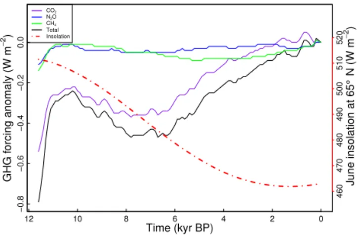
We included the major climatic forcings in terms of green-house gases (GHGs) in the atmosphere, astronomical param-eters (orbital forcing, or ORB) and decaying ice sheets. In all simulations, the solar constant, aerosol levels, the continental configuration and bathymetry were kept fixed at preindus-trial values. We based the concentrations of CO2, CH4and
N2O on ice core measurements for GHG forcing
(Louler-gue et al., 2008; Schilt et al., 2010). The radiative GHG forcing anomaly (relative to 0 kyr) in W m−2(Ramaswamy
et al., 2001), representing the overall GHG contribution, at first showed a rapid rise with a peak of −0.3 W m−2 at
10 kyr, which was followed by a slight decrease towards a minimum at 7 kyr, and gradually increased towards 0 kyr
12 10 8 6 4 2 0
−0.8
−0.6
−0.4
−0.2
0.0
Time (kyr BP)
GHG f
orcing anomaly (W m
−
2)
CO2
N2O CH4
Total Insolation
460
470
480
490
500
510
520
J
u
n
e
i
n
s
o
la
ti
o
n
a
t
6
5
°
N
(
W
m
)
−
2
Figure 1. Evolution of greenhouse gas concentrations (GHGs)
shown as the radiative forcing’s deviation from the preindustrial level (with solid lines corresponding to the left axis), and June
inso-lation at 65◦N derived from orbital configuration (with red line and
the axis on the right).
(Fig. 1). The astronomical parameters (eccentricity, obliq-uity and longitude of perihelion) determine the incoming so-lar radiation at the top of atmosphere and were derived from Berger (1978). An example of the resulting change in inso-lation is shown as the anomaly for June at 65◦N in Fig. 1,
which shows the gradual decrease over the course of the Holocene. While the global annual mean insolation stayed at almost the same level (not shown), both changes in obliq-uity and precession are resulting in insolation variations on the multi-millennial timescale of the Holocene. At the begin-ning of the Holocene (11.5 kyr), the orbitally induced inso-lation anomaly in the NH was positive in summer and nega-tive in winter (Fig. S1 in the Supplement). Overall, this setup of GHG and ORB forcing is in line with the PMIP3 pro-tocol ((http://pmip3.lsce.ipsl.fr), except that our simulation excluded the increase in GHG levels during the industrial era (Ruddiman, 2007). Accordingly, the terms preindustrial (era) and 0 kyr are considered equivalent in the present text and in-dicate modern conditions without anthropogenic impacts.
● ●
● ●
●
●
● ●
● ●
●
●
●
● ●
● ● ●
● ●
11 10 9 8 7
0
10
20
30
40
50
60
Ice sheet area and max thickness
Time (kyr BP)
Area of ice sheets (10E+5 km
2 )
● ● ●
● ●
● ●
● ●
●
● ●
● ●
●
● ● ●
●
● ●
● LIS_size FIS_size LIS_tck FIS_tck
0
500
1000
1750
2500
Max thickness of ice sheets (m)
(a)
11 10 9 8 7
0
20
40
60
80
100
Meltwater flux
Time (kyr BP)
Fresh w
ater in mSv
FWF_1 FWF_2 Fennoscandian St.Law. River Hudson Greenland
(b)
11 10 9 8 7
Equivalent sea level
Time (kyr BP)
−50
−40
−30
−20
−10
0
Sea le
vel (in m) relativ
e to 0kyr
(c)
FWF_v1 FWF_v2 FWF_v1 FWF_v2
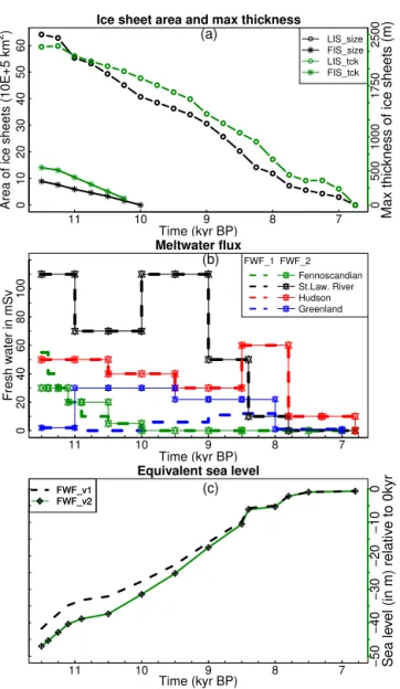
Figure 2. The prescribed ice-sheet forcing during the early
Holocene.(a)Variation in ice-sheet extent (km2) displayed as the
black lines with the axis on the left and their maximum thickness (m) indicated by the green lines with the axis on the right. A rel-atively minor change in GIS is not shown due to its small scale.
(b)Two freshwater flux scenarios (in mSv), FWF-v1 (thick dashed
lines) and FWF-v2 (solid lines).(c)Total meltwater discharge in
equivalent sea level (m).
2010), which is comparable with the ICE-5G reconstruction (Peltier, 2004). Both the spatial extent of the ice sheets and their thickness were updated every 250 years in our transient experiments, and they decreased rapidly during the earliest Holocene, followed by a more gradual deglaciation rate from 8 kyr onward (Fig. 2a).
We applied the meltwater release for 1200 years in our equilibrium experiments for 11.5 kyr by adding 0.11 Sv (1 sverdrup is 106m3s−1) of freshwater at the St. Lawrence
River, 0.05 Sv at Hudson Strait and Hudson River, 0.055 Sv coming from the FIS, and 0.002 Sv from the GIS
(Liccia-rdi et al., 1999; Jennings et al., 2015). The total freshwa-ter volume added to the oceans in our transient experiments was about 1.46×10¹⁶m−3in the first 4700 years (Fig. 2b),
which roughly matches the estimated ice-sheet melting vol-ume during the early Holocene (Dyke et al., 2003; Ganopol-ski et al., 2010; Clark, unpublished data). The volume of meltwater was slightly lower than the volume of the esti-mated 60 m sea level rise that took place during the early Holocene (Fig. 2c) (Lambeck et al., 2014), which suggests a coeval Antarctic melting contribution that is not considered here. Given the lack of a direct imprint left by meltwater on terrestrial records and hence the relatively large uncertainty, we used two versions of the freshwater flux (thick dashed lines and solid lines with symbols in Fig. 2b) that repre-sent two possible deglaciation scenarios of the GIS and FIS, named FWF-v1 and FWF-v2. The GIS FWF_v1 scenario is derived from the ICE_5G reconstruction, and FWF_v2 is based on the reconstruction of Vinther et al. (2009), which suggests a faster GIS thinning. The two FIS freshwater flux (FWF) scenarios are based on two estimations of the FIS melting, since the recent cosmogenic dating (FWF_v2) sup-ports a faster melting (Clark, unpublished data) than previ-ously thought (FWF_v1). However, we kept the freshwater discharge from LIS the same as in version 1, since the LIS deglaciation has been relatively well studied and we are more certain about its contribution.
2.3 Setup of experiments
We performed two types of experiments: equilibrium and transient simulations. First, the equilibrium experiments of OG11.5 and OGIS11.5 with boundary conditions for 11.5 kyr (Table 1) were designed. The OGIS11.5 experiment included ice-sheet forcing, whereas no ice sheets were included in OG11.5 (Table 2). Each of these experiments was initiated from the model’s default modern condition and was run for 1200 years, of which the last 200 years of data was used for the analysis. Renssen et al. (2006) demonstrated that a 1200-year spin-up is sufficient to reach a quasi-equilibrium in all components of the model.
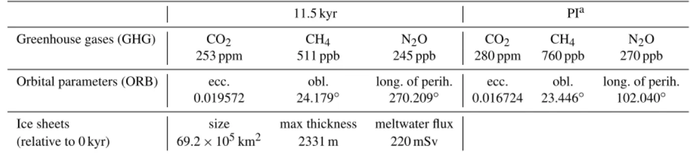
Table 1.Boundary conditions for 11.5 kyr and the preindustrial (PI) era
11.5 kyr PIa
Greenhouse gases (GHG) CO2 CH4 N2O CO2 CH4 N2O
253 ppm 511 ppb 245 ppb 280 ppm 760 ppb 270 ppb
Orbital parameters (ORB) ecc. obl. long. of perih. ecc. obl. long. of perih.
0.019572 24.179◦ 270.209◦ 0.016724 23.446◦ 102.040◦
Ice sheets size max thickness meltwater flux
(relative to 0 kyr) 69.2×10⁵km2 2331 m 220 mSv
PIa: GHG for AD 1750; ORB for AD 1950.
Table 2.Experiments and corresponding setup.
Equilibrium Transient
Name Forcing Name Forcing
OG11.5 ORB+GHG ORBGHG ORB+GHG
OGIS11.5 ORB+GHG+IS+FWFa OGIS_FWF_v1 ORB+GHG+IS+FWF_v1
OGIS_FWF_v2 ORB+GHG+IS+FWF_v2
FWFa: only one freshwater scenario is considered in the OGIS11.5 equilibrium experiment.
with the boundary conditions that are shown in Table 1 and, similarly to the other equilibrium experiments, the results of the last 200 years were used as a reference. These simula-tions and their forcings are summarized in Table 2. All tem-perature values in this study are shown as deviations from the PI simulation (indicates the climate at 0 kyr). Tempera-tures presented here are simulated near-surface temperature values without the environmental lapse rate corrections to the sea level temperature, which imply approximately a 0.5◦C
cold bias over ice-sheet covered regions when compared with site-specific proxy records.
3 Results
3.1 Equilibrium experiments at the onset of the Holocene
3.1.1 Simulation with only ORB and GHG forcings at 11.5 kyr (OG11.5)
In the experiment OG11.5, summer temperatures were 2– 4◦C higher over most of the extratropical continents than
in the PI simulation, with a maximum deviation of 5◦C
in the central parts of the Northern Hemisphere continents (Fig. 3a). The warming over the oceans was about 1.5◦C,
and less conspicuous than that over the continents. These warmer conditions were caused by the orbitally induced pos-itive summer insolation anomaly, as all atmospheric green-house gas levels were lower at 11.5 kyr than in the prein-dustrial era (Fig. 1). The most obvious feature of simulated winter temperatures was the marked contrast between high
latitudes and areas more to the south (Fig. 3b). For instance, midlatitudes were 1.5–3◦C cooler with the strongest
cool-ing in the central continents, whereas the high-latitude Arctic was clearly warmer with a maximum up to+3◦C than the PI.
This latitudinal gradient can be seen in annual mean temper-atures as well (Fig. 3c). Annual mean tempertemper-atures over the Arctic were about 1–4◦C higher than the PI. The warming
was slightly larger in winter than in summer, and this sea-sonal difference mirrors the Arctic Ocean damping effect on a seasonal signal due to a large heat capacity. Temperatures at lower latitudes were annually unchanged (mostly within
±0.5◦C) with a stronger seasonality (with warmer summers
and cooler winters), which is consistent with the insolation change at 11.5 kyr (Fig. S1).
3.1.2 Climate response to melting ice sheets at 11.5 kyr (OGIS11.5)
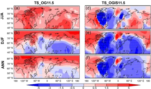
Our simulation OGIS11.5 (including the impact of ice sheets) suggests a much cooler climate than that of OG11.5. Most notably, ice sheets induced a strong summer cooling over ice-covered areas, and reduced temperatures up to 5◦C
compared to the PI simulation, with the strongest cooling at the center of the LIS (Fig. 3d). Additionally, SSTs were also more than 1.5◦C lower over the North Atlantic Ocean.
Figure 3.Simulated temperatures for 11.5 kyr, shown as deviation from the PI. Left column shows the simulation with only GHG and ORB forcings (OG11.5). For the right column, the ice-sheet forcing is included (OGIS11.5). Upper, middle and lower panels present summer (JJA), winter (DJF) and annual mean temperatures, respectively.
Alaska was the only continental region where winter tem-peratures exceeded the preindustrial values by up to+3◦C.
The strongest cooling effect was present in the regions cov-ered by ice sheets, for instance more than 3◦C cooler over
the LIS. Simulated annual mean temperatures in OGIS11.5 clearly showed overall lower values than the PI due to the ice-sheet impacts (Fig. 3f). The Eurasian continent was mostly 1.5–3◦C cooler, and a maximum temperature reduction of
more than 5◦C was found over the LIS. Only two areas were
still warmer: Alaska, including the adjacent sector of the Arc-tic Ocean, and the Nordic Seas. The most distinct feature was thus a thermally contrasting pattern over North Amer-ica, with simulated temperatures being around 2◦C higher
than those the PI for Alaska, whereas over most of Canada temperatures were more than 3◦C lower.
3.2 Transient simulation for the Holocene
It is clear in our analysis of Sect. 3.1 that the climate showed different responses in the following areas: the Arctic, northwestern Europe, northern Canada, Alaska and Siberia (marked in Fig. S2). Therefore, these areas were selected for special examination and the temperature evolutions of these regions will be shown. Our major focus was on millennial-scale temperature trends; therefore, we applied a 500-year running mean to our simulated time series that effectively filtered out high-frequency variability.
3.2.1 Temperature evolution in the Arctic
Arctic summer temperatures in ORBGHG continuously de-creased, which resulted in a total cooling of 2◦C during
the Holocene (Fig. 4). Winter temperatures showed an even stronger overall cooling of−3◦C.
The simulation OGIS_FWF-v1 with full forcings reveals a more complicated Arctic climate evolution compared to that of ORBGHG. The effect of ice sheets at the onset of the Holocene caused temperatures in both summer and winter to be more than 2◦C lower than those indicated by
ORBGHG. The final deglaciation of the FIS happened at 10 kyr, and the corresponding deglaciation for LIS occurred at 6.8 kyr. Therefore, their cooling effects no longer existed after 6.5 kyr, and all three runs showed similar temperatures after that time. As a consequence, the temperature evolution curve of OGIS_FWF-v1 first showed a warming, with the peak being reached at around 7 kyr, when the cooling effects of the ice sheets had been counterbalanced by the insola-tion anomalies. This was subsequently followed by a gradual cooling that was controlled by a decrease in the orbital forc-ing. Simulated temperatures initially had increased by 6.5 kyr at rate of 0.26, 0.21 and 0.44◦C kyr−1for summer, winter
and annual temperatures, respectively. The larger warming rate in annual mean than in summer and in winter was due to a largest response in the winter half year. The Arctic (here we refer to the region located north of 70◦N) has a large part
of ocean where the maximum response was delayed by a few months (Renssen et al., 2005). The study found the largest re-sponse in the winter half year (especially in fall) due to above delayed response that was ultimately caused by the thermal inertia over the oceans (Renssen et al., 2005). Indeed, this ex-planation was furthermore supported by the simulated large warming rate in fall (up to 0.78◦C kyr−1). The
10 8 6 4 2 0 −1 0 1 2 3
Time (kyr BP)
D e v ia ti o n o f T s − J J A ( °C ) Arctic Warm max ORBGHG OGIS_FWF−v1 OGIS_FWF−v2
Slope=0.26°C kyr−1 (a)
10 8 6 4 2 0
−1
0
1
2
3
Time (kyr BP)
D e v ia ti o n o f T s − D J F ( °C ) ORBGHG OGIS_FWF−v1 OGIS_FWF−v2
Slope=0.21°C kyr−1
(b)
10 8 6 4 2 0
−1
0
1
2
3
Time (kyr BP)
D e v ia ti o n o f T s − A N N ( °C ) ORBGHG OGIS_FWF−v1 OGIS_FWF−v2
Slope=0.44°C kyr−1 (c)
Figure 4.Simulated temperature evolution, shown as the anomalies
compared to PI, since the early Holocene at high latitudes (north of
70◦). Panels(a),(b)and(c)represent the summer, winter and
an-nual values, respectively. The slope indicates the overall warming rate and is based on the least-squares regression over the period from the 11.5 to 6 kyr, as from 6 kyr the temperature starts to de-crease. It is only a general estimation, and thus uncertainty ranges are not provided. The warmest peak is marked by a shaded bar and represents the simulated peak during which the temperature was
over 1◦C higher than the PI. Both slope calculation and warm peak
are based on the OGIS_FWF-2 simulation.
by a more gradual warming toward the maximum anomaly of 1◦C warmer than PI at about 7.5 kyr (Fig. 4a). Simulated
winter temperatures stayed at a level of 2◦C lower than that
of ORBGHG before 7 kyr, which was followed by a rapid increase of about 1.5◦C within a 500-year period, and then
reached a temperature peak of about 1.5◦C warmer than the
PI (Fig. 4b). Simulated annual mean temperatures showed a relatively stable rise until 6.5 kyr, which reached a maximum of about 1.5◦C warmer than that of PI (Fig. 4c). The
simu-lation OGIS_FWF-v2 gives similar results for the Arctic but had an even cooler climate before 9 kyr than in OGIS_FWF-v1, with the maximum cooling of up to 0.3◦C for all seasons
at 10.5 kyr.
3.2.2 Temperature evolution in northwestern Europe
The ORBGHG simulation indicates smaller climate variabil-ity in northwestern Europe than in the Arctic. Temperatures declined by around 1.5◦C through the entire period in
sum-10 8 6 4 2 0
−3
−2
−1
0
1
Time (kyr BP)
D e v ia ti o n o f T s − J J A ( °C
) NW Europe
ORBGHG OGIS_FWF−v1 OGIS_FWF−v2 Warm max
Slope=0.28°C kyr−1
(a)
10 8 6 4 2 0
−3 −2 −1 0 1 Time(kyr BP) D e v ia ti o n o f T s − D J F ( °C ) ORBGHG OGIS_FWF−v1 OGIS_FWF−v2
Slope=0.48°C kyr−1
(b)
10 8 6 4 2 0
−3 −2 −1 0 1 Time(kyr BP) D e v ia ti o n o f T s − A N N ( °C ) ORBGHG OGIS_FWF−v1 OGIS_FWF−v2
Slope=0.54°C kyr−1
(c)
Figure 5.Same as Fig. 4 but for northwestern Europe (5◦W–34◦E,
58–69◦N).
mer and less than 0.5◦C for annual mean, and rose by 0.5◦C
in winter (Fig. 5), which implies a decreasing seasonality to-ward the preindustrial era. This contrasts markedly with the clear cooling of climate in each season in the Arctic.
The OGIS_FWF-v1 simulation shows an overall cooler climate in northwestern Europe at the onset of Holocene, with temperature anomalies of−1.5◦C in summer,−3◦C in
winter and−2.8◦C in annual mean compared to the PI
simu-lation. Temperatures increased from this point (11.5 kyr) to-ward 6 kyr at an overall rate of 0.28, 0.48, and 0.54◦C kyr−1
for summer, winter and annual mean, respectively. The most important feature in summer was a sharp temperature rise from a negative anomaly (−1.5◦C) to a positive one (+1◦C)
10 8 6 4 2 0 −6 −4 −2 0 2
Time (kyr BP)
D e v ia ti o n o f T s − J J A ( °C
) N Canada
ORBGHG OGIS_FWF−v1 OGIS_FWF−v2 Warm max
Slope=1.04°C kyr−1
(a)
10 8 6 4 2 0
−6
−4
−2
0
2
Time (kyr BP)
D e v ia ti o n o f T s − D J F ( °C ) ORBGHG OGIS_FWF−v1 OGIS_FWF−v2
Slope=1.08°C kyr−1
(b)
10 8 6 4 2 0
−6
−4
−2
0
2
Time (kyr BP)
D e v ia ti o n o f T s − A N N ( °C ) ORBGHG OGIS_FWF−v1 OGIS_FWF−V2
Slope=1.12°C kyr−1
(c)
Figure 6.Same as Fig. 4 but for northern Canada (120–55◦W, 50–
69◦N).
10 8 6 4 2 0
−1
0
1
2
3
Time (kyr BP)
D e v ia ti o n o f T s − J J A ( °C ) Alaska ORBGHG OGIS_FWF−v1 OGIS_FWF−v2
Slope=−0.30°C kyr−1 (a)
10 8 6 4 2 0
−1
0
1
2
3
Time (kyr BP)
D e v ia ti o n o f T s − D J F ( °C ) ORBGHG OGIS_FWF−v1 OGIS_FWF−v2
Slope=−0.30°C kyr−1 (b)
10 8 6 4 2 0
−1
0
1
2
3
Time (kyr BP)
D e v ia ti o n o f T s − A N N ( °C ) ORBGHG OGIS_FWF−v1 OGIS_FWF−V2
slope=−0.18°C kyr−1 (c)
Figure 7.Same as Fig. 4 but for Alaska (170–120◦W, 58–74◦N).
clear thermal maximum in summer for northwestern Europe, which peaked at around 7.4 kyr.
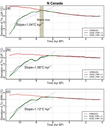
3.2.3 Temperature evolution in northern Canada
Simulated temperatures in ORBGHG for northern Canada decreased by 2.2◦C in summer, by 0.6◦C in winter and by
1.1◦C for annual average during the Holocene (Fig. 6). The
stronger cooling in summer than in winter reflected a strong early Holocene seasonality, which decreased over the whole period.
The OGIS_FWF-v1 simulation describes a much cooler climate in northern Canada during the early Holocene than that indicated by ORBGHG. This cooling was up to 5◦C
for all seasons at the onset of Holocene. The climate dra-matically warmed with an overall high rate of more than 1◦C kyr−1 in both winter and summer during the early
Holocene, which was due to the impact of the decaying LIS. The early Holocene warming was, however, not linear be-cause an initial phase with more rapid warming was fol-lowed by a more gradual temperature increase. In summer, this warming resulted in a thermal peak at around 7.4 kyr, which was about 1.5◦C warmer than the PI. From 7.4 kyr
onwards, the climate experienced a gradual cooling that was very similar to that of ORBGHG. Simulated temperatures in winter and annual mean did not show such a clear warm peak in comparison to summer. The results of OGIS_FWF-v2 only indicated marginal differences relative to OGIS_FWF-v1 for all seasons. Overall, the most significant feature of simulated temperatures in northern Canada was the strong warming that took place in the early Holocene.
3.2.4 Temperature evolution in Alaska
The ORBGHG simulation shows an overall cooling in Alaska for all seasons. Simulated summer and annual mean temperatures experienced a decrease of more than 2◦C throughout the whole period. Winter temperatures had
slightly increased by 10 kyr, and then stayed about 2◦C
higher for a period of 800 years, which was followed by a constant decrease toward the preindustrial value.
In contrast to other areas, both summer and winter temperatures in OGIS_FWF-v1 showed an overall cooling trend in Alaska during the entire Holocene (Fig. 7), which was slightly higher than in our ORBGHG simulation. The OGIS_FWF-v1 simulation indicates a 2◦C decline in
sum-mer temperature over the whole period, with a slightly faster rate between 7 and 6.5 kyr. Simulated winter temperatures decreased by 3.5◦C during the early Holocene, with two
small declines at 9.5 and 6.7 kyr. Annual temperatures in the OGIS_FWF-v1 simulation reflected a 2.3◦C cooling during
3.2.5 Temperature evolution in Siberia
The ORBGHG simulation describes an almost 2◦C
de-cline of summer temperatures over Siberia during the last 11.5 thousand years (Fig. 8). Simulated winter temperatures showed a smaller variation, as it decreased by less than 1◦C,
and annual mean temperatures decreased by around 1◦C
over the course of the Holocene. The evolution of simu-lated temperatures in ORBGHG over Siberia was on a similar scale to that of northwestern Europe.
The difference of simulated Siberian temperatures be-tween ORBGHG and OGIS_FWF-v1 varied in summer and winter. On the one hand, simulated summer temperatures in OGIS_FWF-v1 were generally similar to that in OR-BGHG with the exception of a small warming of 0.7◦C
be-fore 10 kyr. On the other hand, winter temperatures in the OGIS_FWF-v1 simulation were around 2◦C lower than in
ORBGHG before 7 kyr, followed by a rapid increase over the next 500 years, after which it followed the ORBGHG simulation. Consequently, simulated early Holocene warm-ing lasted much longer in winter than in summer. Simulated Siberian temperature evolution in OGIS_FWF-v2 generally followed that of OGIS_FWF-v1.
4 Discussion
We will evaluate our results by briefly comparing the simu-lations with proxy-based reconstructions, which will be fol-lowed by an analysis of the mechanism behind the simulated temperature patterns. The impact of freshwater forcing will also be discussed based on the two FWF scenarios.
4.1 Comparison of simulations with proxy records
At the onset of the Holocene, the overall cool climate indi-cated by the reconstructions generally matches that of our OGIS11.5 simulation, which shows lower annual tempera-tures at 11.5 kyr than the PI. Climate reconstructions based on proxy data generally show a cooler early Holocene over northern Europe than at 0 kyr both in the summer and win-ter (Heiri et al., 2104; Mauri et al., 2015). Terrestrial and ocean sediment data also suggest a cooler early Holocene climate over eastern Siberia (Klemm et al., 2013; Tarasov et al., 2013) and slightly lower SSTs over the North Atlantic Ocean (Came et al., 2007; Berner et al., 2008). Cooler condi-tions over the Barents Sea and Greenland are also indicated by multiple proxies (Peros et al., 2010; de Vernal et al., 2013; Vinther et al., 2008). Therefore, these proxy data agree with simulated lower temperatures over these areas.
However, there is less agreement with proxies in places where the reconstructions are sparse. The only available pollen-based reconstruction from the western side of the Ural Mountains suggests similar early Holocene summer temper-atures (within 1◦C anomaly) compared to the preindustrial
era (Salonen et al., 2011), whereas OGIS11.5 indicates that
10 8 6 4 2 0
−3
−2
−1
0
1
2
Time (kyr BP)
D
e
v
ia
ti
o
n
o
f T
s
−
J
J
A
(
°C
) Siberia
ORBGHG OGIS_FWF−v1 OGIS_FWF−v2
Slope=0.43°C kyr−1
Warm max
(a)
10 8 6 4 2 0
−3
−2
−1
0
1
2
Time (kyr BP)
D
e
v
ia
ti
o
n
o
f T
s
−
D
J
F
(
°C
)
ORBGHG OGIS_FWF−v1 OGIS_FWF−v2
Slope=0.25°C kyr−1 (b)
10 8 6 4 2 0
−3
−2
−1
0
1
2
Time (kyr BP)
D
e
v
ia
ti
o
n
o
f T
s
−
A
N
N
(
°C
)
ORBGHG OGIS_FWF−v1 OGIS_FWF−V2
Slope=0.36°C kyr−1
(c)
Figure 8.Same as Fig. 4 but for Siberia (62–145◦E, 58–74◦N)
and the warming rate slope is indicated for a shorter period (11.5– 9.8 kyr).
summer temperatures were slightly higher at 11.5 kyr over most areas. At high latitudes, the sea-ice cover reconstruc-tions serve as an indirect paleotemperature proxy due to the scarcity of temperature records, and reveal an inconclusive temperature signal over the Canadian Arctic (de Vernal et al., 2013), whereas our simulation reflects an overall warmer climate in the west and cooler conditions in the east.
main temperature features indicated in proxy-based recon-structions.
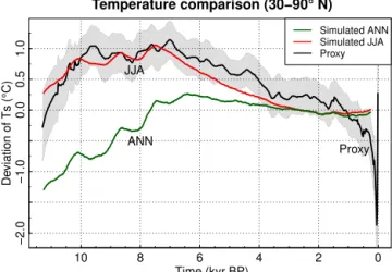
Shakun et al. (2012) and Marcott et al. (2013) stacked multiple proxies to construct a record of temperatures since the LGM. Both above stacked reconstructions and our sim-ulation OGIS_FWF-v2 show that the Holocene was gen-erally characterized by an initial warming and subsequent Holocene warm period over the NH extratropics, which in-dicates the broad consistency between simulation and proxy data. However, there are some disagreements related to sea-sonality (Fig. 9). Marcott et al. (2013) interpreted the stacked temperature reconstruction as representative of the annual mean climate, whereas it shows a better agreement with our simulated summer temperature than with annual mean value (Fig. 9). One potential explanation for this seasonal mismatch is that some proxy records have seasonal bias to-ward summer conditions, as has been suggested recently for many marine-based SST reconstructions from high latitudes (Lohmann et al., 2013). Further region-by-region compar-isons of these warming rates with proxy records are beyond the focus of this work and will be dealt with in a future pub-lication.
4.2 Mechanism of climate response to forcings
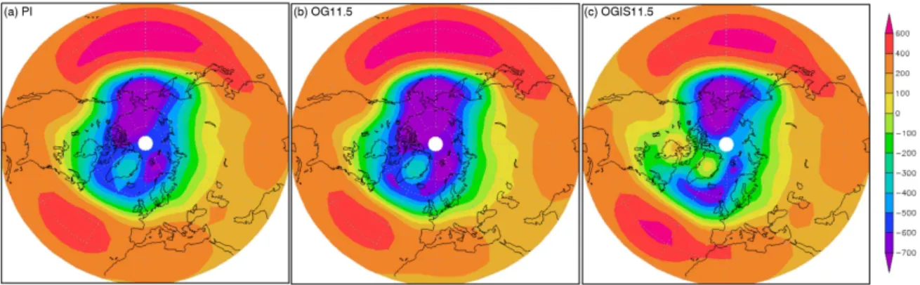
It is clear from our data that the spatial patterns of climate response at the onset of the Holocene can be attributed to the variation in the dominant forcings prevailing in the dif-ferent areas. Orbital-scale insolation variations are impor-tant driving factors for the early Holocene climate. For in-stance, higher temperatures in Alaska could be attributed to the orbitally induced positive insolation anomaly in combi-nation with an anomalous atmospheric circulation caused by the remnant LIS. The air descended over the cold LIS sur-face, which created a high surface pressure anomaly that produced a clockwise flow anomaly at the surface, as indi-cated by the 800 hPa geopotential height (Fig. 10). This in-duces stronger southerly winds over Alaska, which advected relatively warm air from the south. A potentially different early Holocene atmospheric circulation near the North At-lantic was also found in a proxy record of Steffensen et al. (2008), who reported an abrupt transition of deuterium excess that indicates a temperature change of precipitation moisture sources and is thus indirectly connected to atmo-spheric circulation changes.
The strong influence of the ice sheets on early Holocene temperatures has been found in previous studies (Renssen et al., 2009, 2012). Simulated lower summer temperatures over northern Canada and northwestern Europe in our OGIS11.5 simulation were the result of such ice-sheet-induced cooling, which would have fully overwhelmed the warming effect of the positive summer insolation anomaly. The ice-sheet cool-ing effect could partly be explained on a local scale by the enhanced albedo over the ice sheets and by the climate’s high sensitivity to albedo change (Romanova et al., 2006).
10 8 6 4 2 0
−2.0
−1.0
0.0
0.5
1.0
Temperature comparison (30−90° N)
Time (kyr BP)
De
viation of Ts (°C)
Simulated ANN Simulated JJA Proxy
JJA
Proxy ANN
Figure 9.Model–data comparison over the latitudinal band of 30–
90◦N, shown as a deviation from the PI. The stacked temperature
reconstruction with 1δuncertainty (grey band) is based on Marcott
et al. (2013).
Indeed, the summer surface albedo over the ice sheets was much higher (up to 0.8) than over ice-free surfaces, where the values varied from only 0.1 to 0.5, depending on the veg-etation type and the fractional snow cover (Fig. 11). Temper-atures could be further reduced by the ice-sheet orography impact. The elevation of ice sheets introduced descending air over the ice-sheet surface, which caused locally cooler conditions. There was also an approximate 0.5◦C cold bias
induced by the lapse rate effect when compared with the site-based records.
Changes in vegetation and land cover during the early Holocene contributed to climate change as well, especially over ecotonal regions. Modeling studies suggest that defor-estation in boreal regions could decrease regional tempera-tures by up to 1◦C due to an increase in surface albedo and
related positive feedbacks (Levis et al., 1999; Claussen et al., 2001; Liu et al., 2006). Taking Siberia as an example, the insolation-induced warming was partially offset by the over-all higher summer albedo (Fig. 11) induced by the southward expansion of the tundra and/or bare ground and related feed-backs at 11.5 kyr, resulting in a minor warming in summer. The albedo-related feedbacks and the smaller annual insola-tion anomalies jointly result in a 0.5–2◦C cooler in annual
climate at 11.5 kyr. We are aware of the potential role of permafrost at high latitudes; however, the discussion of the impact of permafrost thaw is hindered by the fact that our model version did not include a dynamic permafrost mod-ule. A version of LOVECLIM that is coupled to a permafrost module (VAMPERS) is currently in development (Kitover et al., 2015), and should enable us to quantify the role of per-mafrost in a future study.
Figure 10.Geopotential height anomalies from global mean (in m2s−2) at 800 hPa in the extratropical Northern Hemisphere. Panels(a),
(b)and(c)show the control condition PI and the simulations OG11.5 and OGIS11.5, respectively.
Figure 11.Summer surface albedo in the extratropical Northern Hemisphere. Panels(a),(b)and(c)represent the control run (PI) and the
simulations without ice sheets (OG11.5) and with ice sheets (OGIS11.5), respectively.
with the largest decrease being more than 3 Sv. It was also reflected in a shallower overturning circulation at 11.5 kyr compared to the PI simulation as a response to meltwa-ter release (Fig. 12). This slowdown also coincides with the foraminifera data from the Arctic Ocean and the Fram Strait that suggest a reduced northward oceanic heat trans-port (Thornalley et al., 2009). The slowdown and reduced heat transport led to slightly lower temperatures at high lat-itudes (western Arctic Ocean) at 11.5 kyr than that at 0 kyr. Likewise, after the meltwater fluxes of the LIS diminished around 7 kyr, strong intensification of the AMOC followed. This sudden intensification of AMOC would explain the rapid Arctic temperature increase that occurred at this time (Fig. 4). However, it is important to note that the temperature decrease was not simply inversely linear with the amount of northward transport of heat since the sea-ice feedbacks fur-ther reinforce this change (Roche et al., 2007). In fact, sea-ice coverage in the OGIS11.5 simulation was much more exten-sive over the Davis Strait (northern Labrador Sea) than the corresponding value in OG11.5 (Fig. 13). This extended sea-ice cover in this region was stronger than the direct cool-ing effect of the reduced oceanic heat transport. Such an anomaly might be explained by positive feedbacks involving sea ice being active (Renssen et al., 2005). The Greenland
Sea warming could be attributed to enhanced convective ac-tivity that releases more oceanic heat into the atmosphere. This enhanced convective activity was caused by the shift of deep water formation from the eastern Greenland Sea to the west, which was initially induced by the freshwater discharge from ice-sheet melting. The net response of the climate re-flects the impact of a combination of forcings and feedbacks, which showed a high temporal–spatial variability.
4.3 Early Holocene warming and climate–ocean system response to freshwater
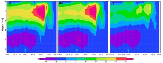
Figure 12.Meridional overturning stream function (Sv) in the Atlantic Ocean basin. Panels(a),(b)and(c)indicate the control run (PI) and the simulations OG11.5 and OGIS11.5, respectively. On the left-hand side, depth is indicated in kilometers. Positive values indicate a clockwise circulation. Maximum AMOC strength value was 22 Sv (reached at about 1200 m depth) in the PI and OGIS simulation, while it was only about 14 Sv (reached at 600–700 m depth) in OGIS11.5.
(a) PI (b) OG11.5 (c) OGIS11.5
Figure 13.Minimum sea-ice thickness (m) in September for PI(a), OG11.5(b)and OGIS11.5(c).
at 10 kyr (Fig. S3) and a sea-ice expansion over the Den-mark Strait (Figs. 14 and S4). However, the efficiency of the above meltwater flux freshening effect is determined by multiple aspects. The most important factor is the maximum flux of meltwater that was added to the ocean, while the to-tal freshwater amount had only a second-order effect (Roche et al., 2007). Numerous investigations on the behavior of the coupled atmosphere–ocean system suggest that the ap-plication of freshwater will not lead to a disruption of the North Atlantic Deep Water production (NADW) as long as a certain threshold is not crossed (Ganopolski et al., 1998; Rahmstorf et al., 2005). Apart from the intensity and dura-tion, the ocean circulation response to freshwater also de-pends on the location where this freshwater is released. For instance, it is more sensitive to the release of freshwater in the eastern Norwegian Sea than at the St. Lawrence River outlet since the former is closer to the main site with NADW formation (Roche et al., 2010). This is consistent with a pre-vious study by Blaschek and Renssen (2103), who found that freshwater from the GIS did have a tangible impact on the Nordic Seas, even though the total amount was minor.
Since the second freshwater scenario (OGIS_FWF-v2) in-cludes a slightly larger FWF from the GIS (compared to that in OGIS_FWF-v1) and the FWF was released in a sensitive area, the location-dependent sensitivity could also partially explain further AMOC weakening in the OGIS_FWF_v2 simulation compared to OGIS_FWF-v1.
10 8 6 4 2 0
12
14
16
18
20
22
24
Time (kyr BP)
Maxim
um AMOC (Sv)
ORBGHG OGIS_FWF−v1 OGIS_FWF−v2
(a)
10 8 6 4 2 0
8.0
9.0
10.0
11.0
Time (kyr BP)
Sea ice in NH (10E+12 m
2)
ORBGHG OGIS_FWF−v1 OGIS_FWF−v2
(b)
Figure 14.Response of the ocean variables (shown as a 100-year
average) to forcings during the Holocene.(a)Maximum meridional
overturning stream function (Sv) in the North Atlantic.(b)Sea-ice
area (1012m2) in the Northern Hemisphere.
northwestern Europe, the OGIS_FWF-v2 represented a more realistic climate than OGIS_FWF-v1 did, which implies that the existing uncertainties in the reconstructions of ice-sheet dynamics can be evaluated by applying different freshwater scenarios. Further comparison with proxy data and with other model transient simulations will be conducted in a future pa-per.
5 Conclusions
We performed both equilibrium and transient simulations by employing the LOVECLIM climate model to explore the spatial patterns of the climate response to forcings at the on-set of the Holocene and temperature evolution over the last 11.5 thousand years. We focused on three research questions in our analysis, which are outlined below with the main find-ing:
1. What were the spatial patterns of simulated temperature at the onset of the Holocene?
The temperature anomalies relative to PI at 11.5 kyr were regionally heterogeneous, which are shown as a range of annually negative anomalies over many areas but which were positive in Alaska. The climate in eastern northern Canada and northwestern Europe was much cooler than in other regions, with temperature anomalies of−2 to−5◦C relative to 0 kyr throughout
the year. The climate over the northern Labrador Sea and the North Atlantic was also 0.5–3◦C cooler.
Temperatures in Siberia were 0.5–3◦C and 1.5–3◦C
lower in winter and annually, respectively, and summer temperatures showed only a small deviation (between
+0.5 and −1.5◦C) compared to 0 kyr. Simulated
summer temperature anomaly in the eastern Arctic Ocean was also small (between+0.5 and−0.5◦C), and
annual temperatures were 0.5–2◦C lower. In contrast to
cooler conditions in other areas, temperatures in Alaska were 1.5–3◦C higher than the preindustrial period for
all seasons.
2. What were the roles of forcings, especially ice-sheet decay, in shaping these features?
The ice-sheet cooling effect in northern Canada and northwestern Europe overwhelmed the warming impact of the positive insolation anomaly, which caused the relatively cold climate at 11.5 kyr. In particular, the enhanced surface albedo over the ice sheets and the orographic effect were important in promoting these cold conditions. The cooler climate over the northern Labrador Sea and the North Atlantic was related to both reduced northward heat transport and enhanced sea-ice feedbacks. A small summer temperature anomaly was found in Siberia, where the positive insolation anomaly was partially offset by the cooling effect of the higher albedo associated with the relatively extensive tundra cover in the early Holocene. Overall, lower winter and annual temperatures at 11.5 kyr over central Siberia can be attributed to both vegetation-related albedo feedbacks and to the relatively small negative insolation deviation compared to the preindustrial level.
The dominant factors driving the climate in eastern Arc-tic Ocean climate were the amount of northward heat transport associated with the strength of ocean circula-tion and the orbitally forced insolacircula-tion variacircula-tion. An-nual mean temperatures at 11.5 kyr were lower than at 0 kyr because the cooling effect of a reduced northward oceanic heat transport (induced by weakened ocean cir-culation) was larger than the insolation-induced warm-ing. During summer, these two factors were of similar magnitude and temperatures were similar to those of the preindustrial era. Temperatures in Alaska were higher for all seasons in response to the dominant positive solation anomaly and the enhanced southerly winds in-duced by the LIS, which advected relatively warm air from the south. Therefore, this regional heterogeneity is the result of the climate response to a range of dominant forcings and feedbacks.
3. What was the spatiotemporal variability in the simu-lated early Holocene evolution?
variability. In contrast, northern Canada experienced a strong warming with an overall warming rate over 1◦C kyr−1, and this warming lasted until 7 kyr.
Al-though different forcings and mechanisms played different roles in northwestern Europe, the Arctic and Siberia, the overall warming effect was similar for these regions, with a rate of around 0.5◦C kyr−1. In addition,
the comparison of early Holocene temperatures over northwestern Europe with proxy records suggests that the OGIS_FWF-v2 represented a more realistic climate condition than the OGIS_FWF-v1 does, and it implies that the uncertainties with regard to the ice-sheet decay can potentially be constrained by applying different deglaciation scenarios and comparing then with networks of proxy records. Overall, our results demonstrated a large spatial variability in the climate response to diverse forcings and feedbacks, both for the early Holocene temperature distribution and for the early Holocene warming, and this data–model comparison also helps in understanding the difference between proxy records.
The Supplement related to this article is available online at doi:10.5194/cp-12-1119-2016-supplement.
Acknowledgements. This work was funded by the China
Schol-arship Council. We would like to thank Didier Roche for helping us to set up the experiments. The constructive comments of the two anonymous reviewers and the editor are gratefully acknowledged.
Edited by: M.-F. Loutre
References
Abe-Ouchi, A., Saito, F., Kawamura, K., Raymo, M. E., Okuno, J., Takahashi, K., and Blatter, H.: Insolation-driven 100 000-year glacial cycles and hysteresis of ice-sheet volume, Nature, 500, 190–193, doi:10.1038/nature12374, 2013.
Berger, A.: Milankovitch Theory and Climate, Rev. Geophys.., 26, 624–657, 1988.
Berger, A. L.: Long-term variations of daily insolation and Quater-nary climatic changes, J. Atmos. Sci., 35, 2362–2367, 1978. Berner, K. S., Koç, N., Divine, D., Godtliebsen, F., and Moros, M.:
A decadal-scale Holocene sea surface temperature record from the subpolar North Atlantic constructed using diatoms and statis-tics and its relation to other climate parameters, Paleoceanogra-phy, 23, PA2210, doi:10.1029/2006pa001339, 2008.
Bigelow, N. H., Brubaker, L. B., Edwards, M. E., Harrison, S. P., Prentice, I. C., Anderson, P. M., Andreev, A. A., Bartlein, P. J., Christensen, T.R., Cramer, W., Kaplan, J. O., Lozhkin, A. V., Matveyeva, N. V., Murray, D. F., McGuire, A. D., Razzhivin, V. Y., Ritchie, J. C., Smith, B., Walker, D.A., Gajewski, K., Wolf, V., Holmqvist, B. H., Igarashi, Y., Kremenetskii, K., Paus, A.,
Pisaric, M. F. J., and Volkova, V. S.: Climate change and Arctic
ecosystems: Vegetation changes north of 55◦N between the last
glacial maximum, mid-Holocene, and present, J. Geophys. Res., 108, 8170, doi:10.1029/2002JD002558, 2003.
Birks, H. H: South to north: Contrasting late-glacial and early-Holocene climate changes and vegetation responses between south and north Norway, Holocene, 25, 37–52, doi:10.1177/0959683614556375, 2015.
Blaschek, M. and Renssen, H.: The Holocene thermal maximum in the Nordic Seas: the impact of Greenland Ice Sheet melt and other forcings in a coupled atmosphere-sea-ice-ocean model, Clim. Past, 9, 1629–1643, doi:10.5194/cp-9-1629-2013, 2013. Bond, G., Broecker, W., Johnsen, S., McManus, J., Labeyrie, L.,
Jouzel, J., and Bonani, G.: Correlations between climate records from North Atlantic sediments and Greenland ice, Nature, 365, 143–147, doi:10.1038/365143a0, 1993.
Brooks, S. J. and Birks, H. J. B.: Chironomid-inferred Late-glacial and early Holocene mean July air temperatures for Krakenes Lake, western Norway, J. Paleolimnol., 23, 77–89, 2000. Brooks, S. J., Matthews, I. P., Birks, H. H., and Birks, H.
J. B.: High resolution Lateglacial and early-Holocene sum-mer air temperature records from Scotland inferred from chironomid assemblages, Quaternary Sci. Rev., 41, 67–82, doi:10.1016/j.quascirev.2012.03.007, 2012.
Brovkin, V., Ganopolski, A., and Svirezhev Y.: A continuous climate-vegetation classification for use in climate-biosphere studies, Ecol. Model., 101, 251–261, 1997.
Buizert, C., Gkinis, V., Severinghaus, J. P., He, F., Lecavalier, B. S., Kindler, P., Leuenberger, M., Carlson, A. E., Vinther, B., Masson-Delmotte, V., White, J. W. C., Liu, Z., Otto-Bliesner, B., and Brook, E. J.: Greenland temperature response to climate forcing during the last deglaciation, Science, 345, 1177–1180, doi:10.1126/science.1254961, 2014.
Came, R. E., Oppo, D. W., and McManus, J. F.: Amplitude and timing of temperature and salinity variability in the subpo-lar North Atlantic over the past 10 kyr, Geology, 35, 315–318, doi:10.1130/g23455a.1, 2007.
CAPE project members, Holocene paleoclimate data from the arctic: Testing models of global climate change, Quaternary Sci. Rev., 20, 1275–1287, doi:10.1016/S0277-3791(01)00010-5, 2001.
Carlson, A. E., Winsor, K., Ullman, D. J., Brook, E., Rood, D. H., Axford, Y., Le Grande, A. N., Anslow, F., and Sinclair, G.: Earliest Holocene south Greenland ice-sheet retreat within its late-Holocene extent, Geophys. Res. Lett., 41, 5514–5521, doi:10.1002/2014GL060800, 2014.
Claussen, M., Brovkin, V., and Ganopolski, A.: Biogeophysical ver-sus biogeochemical feedbacks of large-scale land cover change, Geophys. Res. Lett., 28, 1011–1014, doi:10.1029/2000gl012471, 2001.
Dansgaard, W., Johnsen, S. J., Clausen, H. B., Dahl-Jensen, D., Gundestrup, N. S., Hammer, C. U., Hvidberg, C. S., Steffensen, J. P., Sveinbjornsdottir, A. E., Jouzel, J., and Bond, G.: Evidence for general instability of past climate from a 250 kyr ice-core record, Nature, 364, 218–220, 1993.
de Vernal, A., Hillaire-Marcel, C., Rochon, A., Fréchette, B., Henry, M., Solignac, S., and Bonnet, S.: Dinocyst-based recon-structions of sea ice cover concentration during the Holocene in the Arctic Ocean, the northern North Atlantic Ocean and its adjacent seas, Quaternary Sci. Rev., 79, 111–121, doi:10.1016/j.quascirev.2013.07.006, 2013.
Dyke, A. S., Moore, A., and Robertson, L.: Deglaciation of North America, Open-file report-geological survey of Canada, Canada, 2003.
Fang, K., Morris, J. L., Salonen, J. S., Miller, P. A., Renssen, H., Sykes, M. T., and Seppä, H.: How robust are Holocene treeline simulations? A model-data comparison in the Euro-pean Arctic treeline region, J. Quaternary Sci., 28, 595–604, doi:10.1002/jqs.2654, 2013.
Felzer, B., Oglesby, R. J., Webb, T., and Hyman, D. E.: Sensitiv-ity of a general circulation model to changes in northern hemi-sphere ice sheets, J. Geophys. Res.-Atmos., 101, 19077–19092, doi:10.1029/96JD01219, 1996.
Fichefet, T. and Maqueda, M. A. M.: Sensitivity of a global sea ice model to the treatment of ice thermodynamics and dynamics, J. Geophys. Res., 102, 12609–12646, doi:10.1029/97jc00480, 1997.
Flato, G., Marotzke, J., Abiodun, B., Braconnot, P., Chou, S. C., Collins, W., Cox, P., Driouech, F., Emori, S., Eyring, V., Forest, C., Gleckler, P., Guilyardi, E., Jakob, C., Kattsov, V., Reason, C., and Rummukainen, M.: Evaluation of Climate Models, in: Cli-mate Change 2013: The Physical Science Basis. Contribution of Working Group I to the Fifth Assessment Report of the Intergov-ernmental Panel on Climate Change, edited by: Stocker, T. F., Qin, D., Plattner, G.-K., Tignor, M., Allen, S. K., Boschung, J., Nauels, A., Xia, Y., Bex, V., and Midgley, P. M., Cambridge Uni-versity Press, Cambridge, United Kingdom and New York, NY, USA, 2013.
Ganopolski, A., Kubatzki, C., Claussen, M., Brovkin, V., and Petoukhov, V.: The influence of vegetation-atmosphere-ocean interaction on climate during the mid-Holocene, Science, 280, 1916–1919, 1998.
Ganopolski, A., Calov, R., and Claussen, M.: Simulation of the last glacial cycle with a coupled climate ice-sheet model of interme-diate complexity, Clim. Past, 6, 229–244, doi:10.5194/cp-6-229-2010, 2010.
Goosse, H. and Fichefet, T.: Importance of ice-ocean interactions for the global ocean circulation: A model study, J. Geophys. Res., 23, 337–355, doi:10.1029/1999jc900215, 1999.
Goosse, H., Brovkin, V., Fichefet, T., Haarsma, R., Huybrechts, P., Jongma, J., Mouchet, A., Selten, F., Barriat, P.-Y., Campin, J.-M., Deleersnijder, E., Driesschaert, E., Goelzer, H., Janssens, I., Loutre, M.-F., Morales Maqueda, M. A., Opsteegh, T., Mathieu, P.-P., Munhoven, G., Pettersson, E. J., Renssen, H., Roche, D. M., Schaeffer, M., Tartinville, B., Timmermann, A., and Weber, S. L.: Description of the Earth system model of intermediate complex-ity LOVECLIM version 1.2, Geosci. Model Dev., 3, 603–633, doi:10.5194/gmd-3-603-2010, 2010.
Grootes, P. M., Stuiver, M., White, J. W. C., Johnsen, S., and Jouzel, J.: Comparison of oxygen isotope records from the GISP2 and GRIP Greenland ice cores, Nature, 366, 552–554, 1993. Hald, M., Andersson, C., Ebbesen, H., Jansen, E.,
Klitgaard-Kristensen, D., Risebrobakken, B., Salomonsen, G. R., Sarn-thein, M., Sejrup, H. P., and Telford, R. J.: Variations in
tem-perature and extent of Atlantic Water in the northern North At-lantic during the Holocene, Quaternary Sci. Rev., 26, 3423–3440, doi:10.1016/j.quascirev.2007.10.005, 2007.
Heiri, O., Brooks, S. J., Renssen, H., Bedford, A., Hazekamp, M., Ilyashuk, B., Jeffers E. S., Lang, B., Kirilova, E., Kuiper, S., Mil-let, L., Samartin, S., Toth, M., Verbruggen, F., Watson, J. E., van Asch, N., Lammertsma, E., Amon-Veskimeister, L., Birks, H. H., Birks, H. J. B., Mortensen, M. F., Hoek, W., Magyari, E., Muñoz Sobrino, C., Seppä, H., Tinner, W., Tonkov, S.,Veski, S., and Lot-ter, A. F.: Validation of climate model-inferred regional temper-ature change for late-glacial Europe, Ntemper-ature Communications, 5, 4914, 1–7, doi:10.1038/ncomms5914, 2014.
Hofer, D., Raible, C. C., Merz, N., Dehnert, A., and Kuhlemann, J.: Simulated winter circulation types in the North Atlantic and Eu-ropean region for preindustrial and glacial conditions, Geophys. Res. Lett., 39, L15805, doi:10.1029/2012GL052296, 2012. Jennings, A., Andrews, J., Pearce, C., Wilson, L., and
Ólfasdótt-tir, S.: Detrital carbonate peaks on the Labrador shelf, a 13–7 ka template for freshwater forcing from the Hudson Strait outlet of the Laurentide Ice Sheet into the subpolar gyre, Quaternary Sci. Rev., 107, 62–80, doi:10.1016/j.quascirev.2014.10.022, 2015. Jones, M. C. and Yu, Z.: Rapid deglacial and early Holocene
expan-sion of peatlands in Alaska, P. Natl. Acad. Sci., 107, 7347–7352, doi:10.1073/pnas.0911387107, 2010.
Justino, F. and Peltier, W. R.: The glacial North Atlantic oscillation, Geophys. Res. Lett., 32, L21803, doi:10.1029/2005GL023822, 2005.
Kandiano, E. S., Bauch, H. A., and Müller, A.: Sea surface temper-ature variability in the North Atlantic during the last two glacial– interglacial cycles: comparison of faunal, oxygen isotopic, and Mg/Ca-derived records, Palaeogeogr. Palaeocl., 204, 145–164, doi:10.1016/s0031-0182(03)00728-4, 2004.
Kaufman, D. S., Ager, T. A., Anderson, N. J., Anderson, P. M., Andrews, J. T., Bartlein, P. T., Brubaker, L. B., Coats, L. L., Cwynar, L. C., Duvall, M. L., Dyke, A. S., Edwards, M. E., Eis-ner, W. R., Gajewski, K., Geirsdottir, A., Hu, F. S., Jennings, A. E., Kaplan, M. R., Kerwin, M. W., Lozhkin, A. V., Mac-Donald, G. M., Miller, G. H., Mock, C. J., Oswald, W. W., Ot-toBliesner, B. L., Porinchuw, D. F., Ruhland, K., Smol, J. P., Steig, E. J., and Wolfe, B. B.: Holocene thermal maximum in the
western Arctic (0–180◦W), Quaternary Sci. Rev., 23, 529–560,
doi:10.1016/j.quascirev.2003.09.007, 2004.
Kaufman D. S., Axford Y. L., Henderson A. C., McKay N. P., Os-wald W. W., Saenger C., Anderson R. S., Bailey H. L., Clegg B., Gajewski K., Hu F. S., Jones M. C., Massa C., Routson C. C., Werner A., Wooller M. J., and Yu Z.: Holocene cli-mate changes in eastern Beringia (NW North America). A sys-tematic review of multi-proxy evidence, Quaternary Sci. Rev., doi:10.1016/j.quascirev.2015.10.021, in press, 2016.
Kitover, D. C., van Balen, R., Roche, D. M., Vandenberghe, J., and Renssen, H.: Advancement toward coupling of the VAMPER
permafrost model within the Earth system modeliLOVECLIM
(version 1.0): description and validation, Geosci. Model Dev., 8, 1445–1460, doi:10.5194/gmd-8-1445-2015, 2015.
Koerner, R. M. and Fisher, D. A.: A record of Holocene summer climate from a Canadian High Arctic ice core, Nature, 343, 630– 631, 1990.
Lambeck, K., Rouby, H., Purcell, A., Sun, Y., and Sambridge, M.: Sea level and global ice volumes from the Last Glacial Maximum to the Holocene, P. Natl. Acad. Sci., 111, 15296–15303, 2014. Langen, P. L. and Vinther, B. M.: Response in atmospheric
circula-tion and sources of Greenland precipitacircula-tion to glacial boundary conditions, Clim. Dynam., 32, 1035–1054, doi:10.1007/s00382-008-0438-y, 2009.
Levis, S., Foley, J. A., and Pollard, D.: CO2, climate, and vegetation
feedbacks at the Last Glacial Maximum, J. Geophys. Res., 104, 31191–31198, doi:10.1029/1999jd900837, 1999.
Licciardi, J. M., Teller, J. T., and Clark, P. U.: Freshwater routing by the Laurentide Ice Sheet during the last deglaciation, mechanism of global climate change at millennial time scales, Geophysical Monograph, 112, 177–201, 1999.
Liu, Z., Notaro, M., Kutzbach, J. E., and Liu, N.: Assessing global vegetation-climate feedbacks from observations, J. Climate, 19, 787–814, doi:10.1175/JCLI3658.1, 2006.
Lohmann, G., Pfeiffer, M., Laepple, T., Leduc, G., and Kim, J.-H.: A model-data comparison of the Holocene global sea surface temperature evolution, Clim. Past, 9, 1807–1839, doi:10.5194/cp-9-1807-2013, 2013.
Loulergue, L., Schilt, A., Spahni, R., Masson-Delmotte, V., Blu-nier, T., Lemieux, B., Barnola, J. M., Raynaud, D., Stocker, T. F., and Chappellaz, J.: Orbital and millennial-scale features of
atmo-spheric CH4over the past 800 000 years, Nature, 453, 383–386,
doi:10.1038/nature06950, 2008.
MacDonald, G. M., Velichko, A. A., Kremenetski, C. V., Borisova, O. K., Goleva, A. A., Andreev, A. A., Cwynar, L. C., Riding, R. T., Forman, S. L., Edwards, T.W. D., Aravena, R., Hammarlund, D., Szeicz, J. M., and Gattaulin, V. N.: Holocene treeline history and climate change across northern Eurasia, Quaternary Res., 53, 302–311, 2000.
Marcott, S. A., Shakun, J. D., Clark, P. U., and Mix, A. C.: A Recon-struction of Regional and Global Temperature for the Past 11 300 Years, Science, 339, 1198–1201, doi:10.1126/science.1228026, 2013.
Mauri, A., Davis, B. A. S., Collins, P. M., and Kaplan, J. O.: The climate of Europe during the Holocene: a gridded pollen-based reconstruction and its multi-proxy evaluation, Quaternary Sci. Rev., 112, 109–127, doi:10.1016/j.quascirev.2015.01.013, 2015. Occhietti, S., Parent, M., Lajeunesse, P., Robert, F., and Govare, É.: Late Pleistocene–Early Holocene decay of the Laurentide Ice Sheet in Québec–Labrador, Developments in Quaternary Sci-ence, 15, 601–630, doi:10.1016/b978-0-444-53447-7.00047-7, 2011.
Opsteegh, J. D., Haarsma, R. J., Selten, F. M., and Kattenberg, A.: ECBILT: A dynamic alternative to mixed boundary conditions in ocean models, Tellus, 50A, 348–367, 1998.
Pausata, F. S. R., Li, C., Wettstein, J. J., Kageyama, M., and Ni-sancioglu, K. H.: The key role of topography in altering North Atlantic atmospheric circulation during the last glacial period, Clim. Past, 7, 1089–1101, doi:10.5194/cp-7-1089-2011, 2011. Peltier, W. R.: Global glacial isostasy and the surface of the ice-age
earth: The ice-5G (VM2) model and grace, Annu. Rev. Earth Pl. Sc., 32, 111–149, 2004.
Peros, M., Gajewski, K., Paull, T., Ravindra, R., and Podritske, B.: Multi-proxy record of postglacial environmental change, south-central Melville Island, Northwest Territories, Canada, Quater-nary Res., 73, 247–258, doi:10.1016/j.yqres.2009.11.010, 2010. Putkinen, N. and Lunkka, J. P.: Ice stream behaviour and deglacia-tion of the Scandinavian Ice Sheet in the Kuittijärvi area, Russian Karelia, Bull. Geol. Soc. Finl., 80, 19–37, 2008.
Rahmstorf, S., Crucifix, M., Ganopolski, A., Goosse, H., Ka-menkovich, I., Knutti, R., Lohmann, G., Marsh, R., Mysak, L. A., Wang, Z., and Weaver, A. J.: Thermohaline circulation hystere-sis: A model intercomparison, Geophys. Res. Lett., 32, L23605, doi:10.1029/2005gl023655, 2005.
Ramaswamy, V., Boucher, O., Haigh, J., Hauglustaine, D., Hay-wood, J., Myhre, G., Nakajima, T., Shi, G.Y., Solomon, S.: Ra-diative forcing of climate change, in: Climate Change 2001: The Scientific Basis. Contribution of Working Group I to the Third Assessment Report of the Intergovernmental Panel on Climate Change, Cambridge Univ. Press, Cambridge, UK and New York, NY, USA, 349–416, 2001.
Rasmussen, S. O., Andersen, K. K., Svensson, A. M., Steffensen, J. P., Vinther, B. M., Clausen, H. B., Siggaard-Andersen, M. L., Johnsen, S. J., Larsen, L. B., Dahl-Jensen, D., Bigler, M., Röthlisberger, R., Fischer, H., Goto-Azuma, K., Hansson, M. E., and Ruth, U.: A new Greenland ice core chronology for the last glacial termination, J. Geophys. Res., 111, D06102, doi:10.1029/2005jd006079, 2006.
Renssen, H., Goosse, H., and Fichefet, T.: Modeling the effect of freshwater pulses on the early Holocene climate: the influence of high frequency climate variability, Paleoceanography, 17, 1020, doi:10.1029/2001PA000649, 2002.
Renssen, H., Goosse, H., Fichefet, T., Brovkin, V., Driesschaert, E., and Wolk, F.: Simulating the Holocene climate evolu-tion at northern high latitudes using a coupled atmosphere-sea ice-ocean-vegetation model, Clim. Dynam., 24, 23–43, doi:10.1007/s00382-004-0485-y, 2005.
Renssen, H., Driesschaert, E., Loutre, M. F., and Fichefet, T.: On the importance of initial conditions for simulations of the Mid-Holocene climate, Clim. Past, 2, 91–97, doi:10.5194/cp-2-91-2006, 2006.
Renssen, H., Seppä, H., Heiri, O., Roche, D. M., Goosse, H., and Fichefet, T.: The spatial and temporal complexity of the Holocene thermal maximum, Nat. Geosci., 2, 411–414, doi:10.1038/ngeo513, 2009.
Renssen, H., Goosse, H., Crosta, X., and Roche, D. M.: Early Holocene Laurentide Ice Sheet deglaciation causes cool-ing in the high-latitude Southern Hemisphere through
oceanic teleconnection, Paleoceanography, 25, PA3204,
doi:10.1029/2009pa001854, 2010.
Renssen, H., Seppä, H., Crosta, X., Goosse, H., and Roche, D. M.: Global characterization of the Holocene Thermal Maximum, Quaternary Sci. Rev., 48, 7–19, doi:10.1016/j.quascirev.2012.05.022, 2012.
Renssen, H., Mairesse, A., Goosse, H., Mathiot, P., Heiri, O., Roche, D.M., Nisanciogly, K. H., and Valdes, P. J.: Multiple causes of the Younger Dryas cold period, Nat. Geosci., 8, 946– 949, 2015.