www.atmos-chem-phys.net/13/12451/2013/ doi:10.5194/acp-13-12451-2013
© Author(s) 2013. CC Attribution 3.0 License.
Atmospheric
Chemistry
and Physics
Airborne observations of trace gases over boreal Canada during
BORTAS: campaign climatology, air mass analysis and
enhancement ratios
S. J. O’Shea1, G. Allen1, M. W. Gallagher1, S. J.-B. Bauguitte2, S. M. Illingworth1, M. Le Breton1, J. B. A. Muller1, C. J. Percival1, A. T. Archibald3, D. E. Oram4, M. Parrington5,*, P. I. Palmer5, and A. C. Lewis6
1School of Earth, Atmospheric and Environmental Sciences, University of Manchester, Oxford Road, Manchester,
M13 9PL, UK
2Facility for Airborne Atmospheric Measurements (FAAM), Building 125, Cranfield University, Cranfield, Bedford,
MK43 0AL, UK
3Centre for Atmospheric Science, University of Cambridge, Cambridge, CB2 1EW, UK
4National Centre for Atmospheric Science, School of Environmental Sciences, University of East Anglia, Norwich,
NR4 7TJ, UK
5School of GeoSciences, The University of Edinburgh, Edinburgh, EH9 3JN, UK
6National Centre for Atmospheric Science (NCAS), University of York, Heslington, York, YO10 5DD, UK *now at: European Centre for Medium-Range Weather Forecasts, Shinfield Park, Reading, RG2 9AX, UK
Correspondence to:S. J. O’Shea (sebastian.oshea@manchester.ac.uk) and G. Allen (grant.allen@manchester.ac.uk)
Received: 30 April 2013 – Published in Atmos. Chem. Phys. Discuss.: 29 May 2013 Revised: 25 October 2013 – Accepted: 14 November 2013 – Published: 19 December 2013
Abstract. In situ airborne measurements were made over eastern Canada in summer 2011 as part of the BORTAS experiment (Quantifying the impact of BOReal forest fires on Tropospheric oxidants over the Atlantic using Aircraft and Satellites). In this paper we present observations of greenhouse gases (CO2 and CH4)and other biomass
burn-ing tracers (CO, HCN and CH3CN), both climatologically
and through case studies, as recorded on board the FAAM BAe-146 research aircraft.
Vertical profiles of CO2 were generally characterised by
depleted boundary layer concentrations relative to the free troposphere, consistent with terrestrial biospheric uptake. In contrast, CH4 concentrations were found to rise with
de-creasing altitude due to strong local and regional surface sources. BORTAS observations were found to be broadly comparable with both previous measurements in the region during the regional burning season and with reanalysed com-position fields from the EU Monitoring Atmospheric Com-position and Change (MACC) project. We use coincident tracer–tracer correlations and a Lagrangian trajectory model
to characterise and differentiate air mass history of inter-cepted plumes. In particular, CO, HCN and CH3CN were
used to identify air masses that have been recently influenced by biomass burning.
Examining individual cases we were able to quantify emis-sions from biomass burning. Using both near-field (< 1 day) and far-field (> 1 day) sampling, boreal forest fire plumes were identified throughout the troposphere. Fresh plumes from fires in northwestern Ontario yield emission factors for CH4 and CO2 of 8.5±0.9 g (kg dry matter)−1 and
(kg dry matter)−1 for CO
2 and 1.8±0.2 and 6.1±1 g (kg
dry matter)−1for CH 4.
1 Introduction
The global burden of greenhouse gases (GHGs) has in-creased significantly over the last century. This has mostly been attributed to growth and changes in anthropogenic emissions (Forster and Ramaswamy, 2007). However, trends in globally averaged concentrations alone are not sufficient to predict future changes in the abundance of GHGs and plan mitigation strategies for emission controls. Therefore, the distribution of GHGs needs to be known at a much finer scale, whilst both sources and sinks must be resolved in terms of their process, temporal and spatial variability (Marquis and Tans, 2008; Dlugokencky et al., 2011).
Biomass burning (BB) has long been known to play an im-portant role in the budgets of a variety of atmospheric trace gases and particles, including GHGs (Crutzen et al., 1979; Seiler and Crutzen, 1980). It is estimated that between 1997 and 2009, global BB released on average 2.0 Pg yr−1of car-bon (C) into the atmosphere (van der Werf et al., 2010). How-ever, there is a large degree of uncertainty and variability in the contributions made by particular regions, both intra- and inter-annually. This is due to the unique and episodic nature of individual fire events and the necessary assumptions inher-ent in the monitoring of such emissions. Broadly, however, it has been suggested (van der Werf et al., 2010) that Africa makes the largest contribution to total C emissions (54 %), followed by South America (15 %). Fires in boreal regions have also been suggested to be responsible for large changes in atmospheric composition. For example, forest fires in Rus-sia alone have been causally linked to the accelerated growth rate of global mean CH4concentrations that was observed in
1998, 2002 and 2003 (Dlugokencky et al., 2001; Langenfelds et al., 2002; Simpson et al., 2006).
Climate change has the potential to further increase the impact of wildfires on trace gas budgets. Canadian boreal fire frequency and annual burn area have shown an upward trend since satellites were first able to monitor fires in the 1970s, which is thought to be due to rising mean summer temper-atures in the region observed over the same period (Gillett et al., 2004). Current research suggests that this trend will continue: estimates using global circulation models suggest that fires in Canada will be 30 % more frequent by 2030 and could be up to 150 % more common by the end of the century (Wotton et al., 2010).
As well as being a major source of greenhouse gases, BB can significantly reduce air quality on local to hemispheric scales, with emissions advected by synoptic weather sys-tems (Damoah et al., 2004). On occasion these long-range transported pollutants can lead to exceedances of air qual-ity standards many 1000s of kilometres from the fire source (Jaffe et al., 2004). BB influence can also dominate the
abun-dance of various volatile organic compounds (VOCs) mea-sured at remote background sites (Lewis et al., 2013). Un-der certain burning and meteorological conditions, vertical mixing can be dramatically enhanced by fires (known as py-roconvection), allowing rapid transport of pyrogenic species and particulates into the upper troposphere/lower strato-sphere (UTLS), resulting in perturbations to the Earth’s ra-diation budget, cloud microphysics and stratospheric chem-istry (Damoah et al., 2006; Cammas et al., 2009). However, much work is still needed to fully understand the relative im-pact of BB on overall atmospheric composition (Wotawa and Trainer, 2000; Monks et al., 2009); a particular area of dis-agreement in the literature is whether BB results in the net production of tropospheric O3(Jaffe and Wigder, 2012;
Par-rington et al., 2013).
The BORTAS (Quantifying the impact of BOReal forest fires on Tropospheric oxidants over the Atlantic using Air-craft and Satellites) project was conceived to investigate the distribution and composition of the outflow from North American BB using a combination of ground-based, aircraft and satellite measurements, and to use chemistry transport models to quantify its impact on tropospheric chemistry. The UK’s Facility for Airborne Atmospheric Measurements (FAAM) BAe-146 research aircraft was deployed to Nova Scotia, Canada, where a number of BB plumes of differing ages were sampled (0 to 10 days). A comprehensive descrip-tion of the motivadescrip-tion for the BORTAS experiment can be found in Palmer et al. (2013), along with a description of the FAAM BAe-146 instrumental payload, a general summary of the flights that took place during BORTAS, and the pre-vailing synoptic meteorological conditions.
This paper presents the in situ observations of CO2 and
CH4that were made using cavity-enhanced absorption
spec-troscopy on the FAAM BAe-146 as part of the BORTAS project. In Sect. 2, we describe measurement techniques and analysis methodologies. Section 3 presents bulk statistics us-ing all available measurements; BORTAS measurements are shown to be in agreement with both previous measurements and modelled concentrations. Section 4 identifies individ-ual biomass burning events where enhancement ratios and emission factors can be quantified. The paper is briefly sum-marised in Sect. 5.
2 Data sources and analysis methodology
2.1 Aircraft sampling
58
56
54
52
50
48
46
Latitude
-90 -80 -70 -60 -50 Longitude
8000
6000
4000
2000
0
Altitude, m
58
56
54
52
50
48
46
Latitude
-90 -80 -70 -60 -50 Longitude
300
250
200
150
100
50
CO, ppb
a)
b)
Fig. 1.The geographic coverage of flights during BORTAS, 12 July
to 3 August, 2011 (excluding the Atlantic transits) colour-coded by (a)altitude and(b)CO as a marker for BB.
shown in Fig. 1. For the majority of the campaign the aircraft was based in Halifax, Nova Scotia (Palmer et al., 2013).
CO2and CH4dry air mole fractions were determined
us-ing an adapted system based on a fast greenhouse gas anal-yser (FGGA) from Los Gatos Research Inc., which uses the cavity-enhanced absorption spectroscopy technique. O’Shea et al. (2013) provide an extensive description of this system along with the associated calibration standards, data process-ing and quality control procedures that were performed. In-flight calibrations were frequently performed using three gas standards, all of which are traceable to the WMO (World Meteorological Organization)-recommended scales for CO2
and CH4 measurements (WMO-X2007 and NOAA 2004).
Through summing all known uncertainties the accuracy of the measurements can be estimated to be±1.28 ppb for CH4
and±0.17 ppm for CO2. This represents less than 0.1 % and
0.05 % of typical background concentrations, respectively. The 1 Hz precision is 2.48 ppb (1σ) for CH4and 0.66 ppm
(1σ) for CO2.
We shall also use concentration data for a range of other trace gases (including those principally emitted by BB) for air mass history as described in Sect. 2.2. This includes
car-bon monoxide (CO), a product and tracer of incomplete com-bustion processes, and hydrogen cyanide (HCN) and acetoni-trile (CH3CN), both key tracers of BB. CO was measured
using a vacuum ultraviolet florescence analyser (AL5002, Aerolaser GmbH, Germany; Gerbig et al., 1999). Precision of the 1 Hz CO measurements is±1.5 ppb at 100 ppb; total uncertainty is estimated to be±2 %.
HCN was monitored using chemical ionisation mass spec-trometry (CIMS), with a limit of detection of 5 ppt and a to-tal uncertainty estimated to be 10 % at 3 s time resolution (Le Breton et al., 2013). CH3CN concentrations were
de-termined using a proton transfer reaction mass spectrometer (PTR-MS), with a 9 to 20 s time response depending on the number of species that are measured, and the CH3CN
mea-surement uncertainty is estimated to be±9 % (Murphy et al., 2010). For a description of all other measurements made on the FAAM BAe-146 refer to Palmer et al. (2013).
2.2 Analysis methodology
In Sects. 3 and 4, we will discuss measurements of various trace gases in the context of their air mass history. To dis-tinguish between air masses we make use of a variety of coincident tracer measurements made on board the FAAM BAe-146. As well as being a tracer for incomplete combus-tion, CO is also produced from the oxidation of hydrocar-bons. Reaction with the hydroxyl radical (OH) is the major atmospheric sink.
HCN and CH3CN are principally emitted to the
atmo-sphere by BB (70–85 % of total emissions for HCN and 90– 95 % for CH3CN; Li et al., 2003) and in contrast to CO have
minimal anthropogenic sources. Ocean uptake and oxidation by OH are the primary and secondary loss mechanisms for both species (de Gouw et al., 2003; Li et al., 2003). CO, HCN and CH3CN all have atmospheric lifetimes of over a
month (de Gouw et al., 2003; Li et al., 2003). It can therefore be assumed that these species are inert dispersive tracers for plumes intercepted when they are less than approximately a week old, since chemical losses over this period should be small. These lifetimes are also short enough so that BB emissions are a substantial increase over the ambient concen-trations. For these reasons all three species are widely used tracers for BB (Hecobian et al., 2011; Hornbrook et al., 2011; Vay et al., 2011).
To allow comparison between species that were measured using different instruments with different response times a number of different data merges were used. When describ-ing the bulk distribution encountered (Sect. 3) 10 s averaged measurements were employed, but when examining the indi-vidual BB case studies (Sect. 4) higher-resolution measure-ments of 3 s were applied. PTR-MS measuremeasure-ments were not used in the 3 s merge.
A common method to identify BB plumes is to use some combination of HCN, CH3CN and CO to partition air masses
recently influenced by biomass burning (Hornbrook et al., 2011; Vay et al., 2011; Palmer et al., 2013). A representa-tive threshold concentration value and/or ratio is chosen from tracer–tracer relationships, where the tracer measurements above a certain threshold value are classified as a biomass burning plume. There are a variety of methods that can be used to choose the threshold, but no consistent method is used within the literature (Le Breton et al., 2013), as the chemical background to each dataset or region may be dif-ferent, requiring unique and tailored analysis. The choice of threshold must also take account plume age, as typical plumes will continuously mix (dilute) with background air until they become indistinguishable from each other. For long-lived species, such as CO2 and CH4, BB will always
make some contribution to their global mean background, further necessitating a tailored approach appropriate to the dataset under analysis.
To probe the history of the air masses encountered by the FAAM BAe-146 we used single-particle 3-dimensional (ver-tical motion enabled) back trajectories from the offline Hy-brid Single-Particle Lagrangian Integrated Trajectory (HYS-PLIT) model (Draxler and Rolph, 2003) with National Cen-ters for Environmental Prediction (NCEP) reanalysis meteo-rological fields at 2.5◦spatial resolution on 17 levels. Five-day back trajectories (with half-hourly outputs) were calcu-lated with endpoints co-located with the aircraft position as reported by GPS at 60 s intervals along the aircraft flight track. This method allows us to qualitatively describe air mass history representative of the aircraft sampling. It should be noted that this method does not represent a source inver-sion and is used here to guide our analysis in terms of quali-tative air mass history and general source regions.
The UK Met Office Numerical Atmospheric-dispersion Modelling Environment (NAME) (Jones et al., 2007) was used to complement the back trajectories generated using HYSPLIT. NAME is a stochastic Lagrangian particle dis-persion model that can be run both forwards and backwards in time. NAME can use single site observations or 3-D me-teorological data to drive the dispersion of the model parti-cles. In this work we have used numerical weather prediction data from the UK Met Office Unified Model (Davies et al., 2005). These are operational analysis fields with a spatial res-olution of 0.35◦longitude by 0.23◦latitude with 59 vertical levels (model top at∼30 km). NAME has previously been used to examine the dispersal of particulate matter originat-ing from Russian agricultural fires and its impact on UK air quality (Witham and Manning, 2007). In this work we per-formed two sets of NAME simulations. The first simulations (not discussed further) were performed in order to simulate the dispersal of the biomass burning plumes that may have influenced our measurements. We focus here on the second set of simulations. These involved releasing 100 000 parti-cles/trajectories over a 1 min period from the locations (lat-itude, long(lat-itude, alt(lat-itude, time) of a selected number of air-craft observations. The locations of the particles were tracked
over a 5-day period going backwards in time. Our analysis focuses on the total column and surface (0 to 200 m a.g.l.) time-integrated latitude–longitude distribution of particles.
3 Results and discussion
3.1 Large-scale distribution
For the purpose of providing a useful dataset for wider clima-tological statistics, we present a broad summary of the BOR-TAS project using all sampled data, excluding the Atlantic transits to Halifax, to represent composition statistics consis-tent with boreal biomass burning that may be linked to satel-lite fire observations. The flights during the BORTAS exper-iment had the explicit aim of intercepting BB, and therefore the measurements discussed here do not represent a truly ran-dom sample of the atmosphere during this measurement pe-riod and will have a slight bias towards air masses that have been influenced by BB.
Observations on board the FAAM BAe-146 during the BORTAS flights are summarised in Fig. 2, and overall cam-paign statistics are shown in Table 1. Notable features of the CO2 altitude profile are the consistently depleted
near-surface concentrations, likely due to uptake by the biosphere. This hypothesis is supported by the enhancements in bio-genic VOCs that generally occurred during periods of CO2
depletion. For example, at low altitudes (< 1000 m) the mean concentration of isoprene (C5H8), which is principally
emit-ted to the atmosphere from terrestrial plants (Guenther et al., 2006), is a factor 6 larger for the lower CO2quartile than it
is for the higher CO2quartile. In contrast to CO2, the
near-surface CH4levels are in general enhanced by several tens of
ppb compared to those aloft, suggesting significant localised and land-based sources in the region.
Pollution events are evident in Fig. 2c–d since CO and CH3CN have many high concentration outliers of an episodic
or transitory nature that are many times larger than the cleaner conditions exhibited in the lower quartile. These ex-treme concentrations, largely associated with BB, are rela-tively evenly distributed across all altitudes, showing that BB not only impacts the region surrounding the fire but is capa-ble of causing changes in composition throughout the tropo-sphere.
Clear evidence for enhancements due to BB can be found in the BORTAS CO2 and CH4 datasets. This is shown in
Fig. 3, where the scatter plots have been colour-coded by CH3CN as a tracer for BB. However, these enhancements
are proportionately quite small compared to their background levels and are obscured by variability in CO2and CH4that is
not associated with changes in CH3CN, suggesting that
ad-ditional (possibly anthropogenic as well as biogenic) fluxes are influencing concentrations. As a consequence the correla-tion with CO across all flights is weak (CO2: COR2=0.09
Table 1.Statistics for all BORTAS flights excluding the transits from Cranfield, UK, to Nova Scotia, Canada, and the return journey.
Mean Median Minimum Maximum PBL mean BB plume mean Background mean
CO2, ppm 384.8 385.1 371.5 397.1 381.3 385.8 383.8
CH4, ppb 1859 1857 1797 1968 1880 1859 1859
1.0 0.0
CH3CN, ppb
8000
6000
4000
2000
0
Altitude, m
1000 0
CO, ppb 8000
6000
4000
2000
0
Altitude, m
1900 1800
CH4, ppb
8000
6000
4000
2000
0
Altitude, m
395 390 385 380 375
CO2, ppm
8000
6000
4000
2000
0
Altitude, m
a) b)
c) d)
Fig. 2. A summary of the observations of CH4, CO2, CO and
CH3CN made on the FAAM BAe-146 during the BORTAS project. The transits from Cranfield, UK, to Nova Scotia, Canada, and the return journey have been excluded from these plots. Boxes are 25th and 75th percentiles, whiskers are 10th and 90th percentiles and the markers are outliers.
of VOCs, where the typical enhancements are several times larger than their background and the influence of BB on the dataset is much more distinct (Lewis et al., 2013).
To analyse the background measurements we filter the dataset for measurements made when the HCN and CH3CN
concentrations are below the median for the campaign, 76 ppt and 137 ppt, respectively. This will remove the influ-ence of BB from all but the smallest and most well mixed plumes to give a confident background concentration. Us-ing this criteria, the correlation between CH4 and CO2 is
much stronger (R2=0.72), giving us good confidence in our
Fig. 3.The relationships between CH4, CO2, CO and CH3CN for
the BORTAS flights with the exception of the Atlantic transits.
choice for the BORTAS dataset. A negative relationship is found with regression slope (−5.31±0.01)×10−3mol CH4
(mol CO2)−1. A negative correlation is consistent with a
combination of CO2 uptake by the biosphere within the
re-gion and surface emissions of CH4. Biogenic CH4-to-CO2
flux ratios have shown a wide degree of variability; for exam-ple ground-based eddy covariance flux measurements found the flux ratio to vary between−56 and−2×10⁻³mol CH
4
(mol CO2)−1 from Californian rice fields over the growing
season (McMillan et al., 2007).
Ethane (C2H6) shares several common sources with
CH4: BB, combustion of fossil fuels and biofuels; however
it does not have a biogenic source. For this reason simultane-ous measurement of C2H6can aid the apportionment of CH4
and CO is much stronger than it is for CH4 (R2=0.95 for
all measurements; Lewis et al., 2013), whilst for both plume and non-plume measurements correlation between C2H6and
CH4 integrated across all flights during BORTAS is poor
(R2< 0.3). However, C2H6: CH4correlation for background
measurements was noted to range widely flight by flight, with a peak of 0.95 during flight B624 (for 8 samples) and a mini-mum of 0.05 for flight B622 (for 5 samples). This would sug-gest that the variability in non-fire (background) CH4
con-centrations is generally due to biogenic emissions. However, it should be noted that the C2H6observations were retrieved
by analysing 529 flask samples, and therefore we do not have equivalent spatial or temporal resolution with the continuous in situ CH4and CO measurements, nor the quantity of
sam-ples from which to fully investigate the relationship to C2H6
in the same way that we are able to do for the 0.1 Hz in situ measurements. Sample locations and times were manually chosen to reflect both plume and background air masses.
Examining bulk statistics for all science flight measure-ments, CO2 and CH4 concentrations made in BB plumes
are only marginally different to those outside of plumes (Ta-ble 1). For CO2 the mean in-plume concentration is only
2 ppm higher than the mean out of plume, and within analyt-ical uncertainty the mean CH4 concentrations are identical.
In Sect. 4 we identify individual case studies in the dataset where enhancements due to BB can be quantified.
As reported by Palmer et al. (2013) fire activity during the BORTAS sampling period was dominated by widespread fires in northwestern Ontario. Extensive fires in this region took place from 17 to 19 July 2011, plumes from which were sampled over 1000 km downwind during measurement flights B621 to B624 (18 to 21 July 2011, Sect. 4.2). This re-gion was also sampled in the near field (plumes < 1 h old) on 26 July 2011 (B626, Sect. 4.1); however, at this time, fire activity in the region was reduced and the plumes more localised. The flights later in the campaign (B628, 28 July 2011) sampled plumes that were reported to be over 7 days old (Parrington et al., 2013). Concentrations in these plumes were relatively low, with CO reaching 135 ppb, HCN 330 ppt and CH3CN 310 ppt; nevertheless the correlation
be-tween HCN and CO (R2=0.69 for the whole flight) implies that they are still representative of a biomass burning origin. As a tracer for incomplete combustion, CO enhancements are characteristic of not only BB but also anthropogenic ac-tivity. Throughout the BORTAS dataset regions of enhanced CO are almost entirely coincident with enhancements in CH3CN (R2=0.89 for all measurements, Fig. 3),
suggest-ing that anthropogenic emissions are well mixed and local sources had a minimal influence on the BORTAS dataset. An exception to this occurred during flight B629, which briefly overflew the Dartmouth Oil refinery located on Halifax Har-bour, NS. Whilst overflying the refinery, CO2was enhanced
by 8 ppm over the local average background and enhance-ments were also noted in NOx (NO up to 3.3 ppb and NO2
up to 3.8 ppb). The high partitioning of NO / NO2 suggests
that this is a photochemically fresh plume and therefore lo-cal in origin. We note that there was no observable significant change in CO and CH4or BB tracers (e.g. CH3CN). 3.2 Comparison with previous observations
On Sable Island, approximately 100 km southeast of Halifax a WMO regional monitoring station makes long-term GHG observations. Given the different sampling domain, the BOR-TAS campaign statistics are comparable to the GHG mea-surements made on Sable Island (WDCGG, 2013). The mean CO2concentration on Sable Island during the BORTAS
sam-pling period was 386.5 ppm, 1.7 ppm higher than the BOR-TAS campaign mean and 5.2 ppm higher than the BORBOR-TAS planetary boundary layer (PBL) mean (Sable Island CO2
statistics: median=385.7 ppm and inter-quartile range 384.2 to 388.5 ppm). The mean CH4concentration on Sable Island
of 1864 ppb is 5 ppb higher than the FAAM BAe-146 mea-surements and 15 ppb lower than the BORTAS PBL mean (Sable Island CH4 statistics: median=1860 ppb and
inter-quartile range 1856 to 1872 ppm).
Two previous airborne measurement campaigns have been performed within a sampling domain, altitude range and time of year similar to BORTAS. These are the 2008 ARCTAS ex-periment (Arctic Research of the Composition of the Tropo-sphere from Aircraft and Satellites, described by Jacob et al., 2010) and the 1992 ABLE-3B experiment (Arctic Boundary Layer Expedition; Harriss et al., 1994). The airborne sam-pling portion of ARCTAS consisted of both spring and sum-mer campaigns over much of the North Asum-merican sub-Artic. During the summer deployment CO2 measurements had a
mean of 382.8±3.0 ppm and median 383.1 ppm, marginally lower than those during BORTAS. However, the ARCTAS project experienced a wider range of concentrations, 368.3 to 624.2 ppm. These very high concentrations were due to sampling intense boreal fires in the near field. Whilst me-dian free-tropospheric CO2values for each altitude bin range
shown in Fig. 2 compare within several ppm to those ob-served during the ARCTAS summer deployment (Vay et al., 2011), BORTAS CH4 concentrations were also found to be
generally similar to those during ARCTAS (Singh et al., 2010), as were other species such as CO and O3(Parrington
et al., 2013). Similar vertical CH4gradients to those shown
in Fig. 2 were observed during ABLE-3B. However, the baseline ABLE-3B CH4 concentrations are approximately
100 ppb lower (Wofsy et al., 1994), reflecting the growth of global CH4 concentrations during the intervening 20 yr
pe-riod between the two projects (Dlugokencky et al., 2011).
3.3 Comparison to MACC model composition
To discuss trace gas measurements as recorded during BOR-TAS in the context of sources of composition model bias, we compared the in situ measurements of CO2, CH4 and
Atmospheric Composition and Change (MACC) project (In-ness et al., 2013). The global MACC reanalysis service pro-vides a reanalysis for the years 2003 to 2012 of trace gas and aerosol concentrations, with the reactive gases reanal-ysis system produced by the coupled Integrated Forecast-ing System–Model for OZone And Related chemical Tracers (IFS-MOZART) modelling and assimilation system. Bene-dictow et al. (2013) give the latest validation report on the MACC reanalysis product.
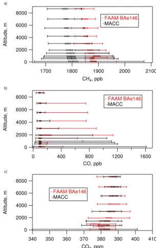
This comparison is shown in Fig. 4. The MACC fields used are statistics that have been determined over the correspond-ing BORTAS measurement period of 18 July to 21 July 2011 for the whole sample region covered by the FAAM BAe-146, excluding the Atlantic transits to and from Cranfield, UK (a geographic region of 40 to 60◦N and 40 to 100◦W). Since
the MACC fields have not been sampled at the exact time and position of the FAAM BAe-146 flights, precise agree-ment between measureagree-ment and model is not expected. How-ever, the comparison is instructive since it tests the model’s skill at simulating the large-scale features and typical back-ground concentrations in the region. For comparison the in situ BORTAS dataset is binned using MACC product altitude levels. It should be pointed out that because of a known bias in the MACC reanalysis dataset for CO2, a different MACC
product was used for CO2in comparison to that used for CO
and CH4. The CO2 fields were produced using a forward
model that is run using optimized fluxes (see Chevallier et al., 2010). The two different products use slightly different pressure levels, which can be seen in Fig. 4, but this does not have an impact on the significance of the comparison as outlined below.
For CO, the MACC is able to reproduce both the high con-centrations from episodic BB events and the approximate background levels with reasonable agreement to the mea-surements. Emission inventories augmented with MODIS (Moderate-Resolution Imaging Spectroradiometer) fire in-formation, as well as CO observations from IASI and MO-PITT, were assimilated during the reanalysis experiment. The mean difference between the medians for individual altitude bins is∼5 ppb (comparable to the total column bias) and the inter-quartile ranges generally agree. The large negative CO biases observed by Inness et al. (2013) are not seen here, possibly because that comparison found the largest discrep-ancies in the boundary layer at urban sites affected by pollu-tion.
Similarly good agreement is seen for CO2where the
me-dian concentrations for each altitude bin are typically within 1 ppm and the inter-quartile ranges are comparable. MACC is also able to simulate the general structure of the CH4
alti-tude profile. However there exists a significant disagreement over the absolute concentrations; MACC typically underes-timates CH4by approximately 75 ppb. This deviation is
suf-ficiently large and consistent in the vertical, such that it is unlikely to be a result of the BORTAS sampling strategy. De-tailed analysis of this disparity is beyond the scope of this
pa-2100 2000
1900 1800
1700
CH4, ppb 8000
6000
4000
2000
0
Altitude, m
- FAAM BAe146
-MACC
1600 1200
800 400
0
CO, ppb 8000
6000
4000
2000
0
Altitude, m
- FAAM BAe146
-MACC
410 400 390 380 370 360 350 340
CO2, ppm
8000
6000
4000
2000
0
Altitude, m
- FAAM BAe146
-MACC
a)
b)
c)
Fig. 4.Comparison between in situ measurements on the FAAM
BAe-146 and those derived from the Monitoring Atmospheric Com-position and Change (MACC) project over the BORTAS sampling domain and period. Boxes are the 25th and 75th percentiles, the whiskers are the maximum and minimum values.
per, but we note the CH4reanalysis data use retrievals from
the SCanning Imaging Absorption SpectroMeter for Atmo-spheric CHartographY (SCIAMACHY) on board the EN-VISAT satellite, which have been produced by the Nether-lands Institute for Space Research (SRON), and that these values are known to have a negative bias (A. Agusti-Panareda and S. Massart, personal communication, 2013)
4 Enhancement ratios and emission factors
Trace gas emissions from biomass burning are often ex-pressed as either an emission ratio (ER) or an emission factor (EF). An ER for a species, X, is the number of molecules of this species emitted into the atmosphere per molecule of a tracer for biomass burning, usually CO2 or CO. It is equal
given are the standard deviation of the fit. Correlation co-efficients (R2) have also been included, which have been calculated using least squares regression. ERs can also be calculated by first subtracting the background concentrations from the in the plume measurements. However we have cho-sen not to use this approach, due to the subjective nature of choosing a background. As a BB plume moves away from its source, chemical reactions may enhance or deplete a partic-ular species and as a consequence the determined ER. For this reason, the ER for short-lived species should only be calculated using measurements in the freshest possible fire plumes. In aged plumes the regression slope is usually known as a normalised excess mixing ratio (NEMR) or enhancement ratio instead (Yokelson et al., 2009; Hecobian et al., 2011; Akagi et al., 2011, 2012; Le Breton et al., 2013; Yokelson et al., 2013).
While an EF is the mass of the species emitted for every kg of dry biomass burnt, it is usually calculated using the carbon mass balance technique (Andreae and Merlet, 2001; Chris-tian et al., 2007; Simpson et al., 2011; Akagi et al., 2012). This is based on the assumption that all combusted carbon (C) is measured in the plume. The EF, in g of X per kg of dry matter burnt, can be calculated using Eq. (1):
EF=FC·
MX1CX
MC1CT
(1) whereFCis the fraction of C in the fuel. For boreal forests
this is chosen to be 500 g kg−1and is thought to be accurate to±10 % (2σ) (Susott et al., 1996; Yokelson et al., 1999).
MXandMCare the molecular masses of species X and
car-bon (12.011 g mol−1), respectively. 1C
X/1CT is the ratio
of the number of moles of species X to the total number of moles of carbon emitted by the fire. This can be cal-culated using the ER, when CO is used as a tracer, of X (1[CX]/1[CO]) and all the other C containing molecules
in the plume. It is not possible to measure all C containing molecules, so we approximate total C using only CO2, CO
and CH4. This will result in an overestimate of the true value,
but this is only expected to amount to a few percent. Simpson et al. (2011) measured CO2, CO, CH4and 80 non-methane
VOCs in Canadian biomass burning plumes and found that 98.6 % of the measured C was either in the form of CO2, CO
or CH4. We can then calculate1CX/1CTusing Eq. (2):
1CX
1CT
=
1[CX] 1[CO]
1+1[CO2] 1[CO] +
1[CH4] 1[CO]
(2)
An emission rate for a species can be estimated by combin-ing its EF with an estimate of the total matter burnt e.g. us-ing The Global Fire Emissions Database (van der Werf et al., 2010). However, a single EF is not sufficient to describe emissions within a particular biome or even an individual fire that will go through several distinct combustion phases with different EFs. A review of the variables that influence the EF is provided by van Leeuwen and van der Werf (2011).
These include factors related to the material burnt (size, den-sity, water content, vegetation spacing) as well as meteoro-logical factors (wind speed, humidity, precipitation, temper-ature). For this reason we include the modified combustion efficiency (MCE, Eq. 3) in Table 2 as a measure of whether a fire is predominantly in the flaming or smouldering phase.
MCE= 1
1− 1[CO]
1[CO2]
(3)
Laboratory studies suggest that this varies from 0.8 for purely smouldering combustion to 0.99 for purely flaming combus-tion (Yokelson et al., 1996).
4.1 Near field biomass burning: 26 July 2011 plume
The flights during the BORTAS project had the aim of sam-pling BB plumes that were a variety of ages. Only Flight B626 (26 July 2011) sampled fresh plumes (< 1 h). This flight consisted of a transit from Halifax, Nova Scotia, followed by a boundary layer survey over an active fire region in north-western Ontario (∼52.5◦N,∼93.6◦W), before landing at Thunder Bay, Ontario. We concentrate our analysis here on the low-level portion of the flight (900 m to 1100 m). Fig-ure 5a shows a time series of BB tracer concentrations whilst repeatedly penetrating a number of plumes, where the BB tracers discussed in Sect. 2 were clearly elevated above their local background.
At such close proximity to the fires the plumes are of lim-ited spatial extent (of the order 1 km), it is therefore ben-eficial to use higher frequency measurements (0.33 Hz) for analysis rather than the 0.1 Hz measurements that have been used previously. We use the method described by LeBreton et al. (2013), using HCN and CO, to determine whether BB has recently influenced an air mass. Firstly, the HCN and CO time series are examined for periods out-of-plume during the low-level flying that represent a typical background. For CO and HCN this was facilitated by relatively large enhance-ments (up to factor 15) in the plume. The mean and stan-dard deviation of the background regions were then deter-mined. Measurements made when the simultaneous CO and HCN mole fraction were 6 standard deviations greater than their background were deemed to be in a BB plume. It should be noted that the measurements are not normally distributed (due to non-random sampling) and as a result no assumption should be made about the proportion of measurements within 1 standard deviation of the mean. The 6 standard deviation threshold is only used to represent a significant enhancement over the background.
Table 2.Emission ratios (ER), normalised excess mixing ratios (NEMR) and emission factors (EF) determined by sampling boreal biomass burning plumes over eastern Canada. MCE is the modified combustion efficiency, a measure of the combustion phase of the fire. The ER and EF determined in this study show good agreement with previous studies in boreal regions. Andreae and Merlet (2001) and Akagi et al. (2011) have compiled values from the literature for extra-tropical forests. Simpson et al. (2011) report values for forest fires in boreal Canada made as part of the ARCTAS project. Units are (mol (mol CO)−1)for the NEMR / ERs and g (kg dry matter)−1for the EFs. Runs are when the aircraft does not change altitude and profiles are when there is a change in altitude.
Flight MCE CO2 CO CH4
ER / NEMR EF ER / NEMR EF ER / NEMR EF
Fresh plume B626 0.83±0.01 5.1±0.3 1512±185 – 189±23 0.079±0.001 8.5±0.9
Aged plumes (> 1 day)
B621 Run 3 0.90±0.01 9.1±0.8 1638±255 – 114±17 0.079±0.004 5.2±0.7
B621 Run 15 – – – – – 0.109±0.003 –
B621 Profile 2 0.90±0.001 9.4±0.2 1648±169 – 111±11 0.05±0.001 3.3±0.3
B621 Profile 3 – – – – – 0.16±0.01 –
B622 Run 1 0.89±0.01 8.1±0.5 1618±216 – 126±17 0.078±0.003 5.7±0.7
B622 Run 3 0.93±0.01 14.4±0.2 1708±173 – 75±8 0.044±0.001 1.8±0.2
B622 Run 6 0.92±0.04 13±7 1683±1400 – 84±73 0.12±0.04 5.9±3.9
B622 Run 9 0.92±0.03 12±5 1679±1000 – 87±53 0.12±0.05 6.1±1
B623 Run 1 and 2 – – – – – 0.133±0.001 –
B623 Run 3 – – – – – 0.093±0.001 –
B623 Run 5 and 6 0.93±0.001 14.2±0.2 1702±173 – 76±8 0.081±0.001 3.5±0.4
Literature values
Andreae and Merlet (2001) – – 1569±131 – 107±37 – 4.7±1.9
Simpson et al. (2011) – 9.1±5.8 1616±180 – 113±72 0.072±0.044 4.7±2.9
Akagi et al. (2011) – – 1489±121 – 127±45 – 6.0±3.1
HCN in the troposphere is not as well known as it is for CO. Mean tropospheric HCN concentrations from previ-ous studies were found to be 243±118 ppt (Singh et al., 2003) and 220 ppt (Li et al., 2003), comparable to the background that we determine. Tracer–tracer scatter anal-ysis of CO2, CH4 and CO measurements are shown in
Fig. 5b and c. For both CO2 and CH4, strongly
corre-lated (R2=0.95 for CH4, and R2=0.69 for CO2) linear
relationships were found for the BB plume measurements as expected. Since the flight traversed across a small re-gion several times, we include all BB plume measurements to calculate a single ER/EF per species for this period. ERs are found to be 0.079±0.001 mol CH4 (mol CO)−1
and 5.9±0.4 mol CO2 (mol CO)−1. From these ERs, using
Eq. (1) and Eq. (2), EFs of 8.5±˙0.9 g (kg dry matter)−1and 1512±185 g (kg dry matter)−1 can be calculated for CH4
and CO2, respectively. Calculated EFs are comparable with
previous studies in boreal regions (see Table 2), as are those for CO and HCN (not shown).
An MCE of 0.83±0.01 is characteristic of smouldering combustion, which would typically result in proportionally more reduced compounds being released. This will likely be the reason for a relatively large amount of CH4 being
re-leased compared to previous studies. van Leeuwen and van der Werf (2011) grouped CH4EFs in the literature based on
biome and the fires’ MCE. The EF calculated for B626 shows an excellent agreement with the amount of CH4emitted for
a fire with its combustion efficiency as predicted from their work.
To examine the sensitivity of the definition of a BB plume on the determined EFs, we repeated the analysis varying the
threshold from 0 to 20 standard deviations above the back-ground. For both CH4and CO2the correlation with CO
in-creases as the threshold rises, as would be expected from removing non-BB sources from the dataset used in the EF calculation. The increase in correlation is more dramatic for CO2than CH4 (for all thresholds the CH4vs. COR2 is
al-ways greater than 0.8). Apart from standard deviation thresh-olds less than 6, the determined EFs are within 10 % of each other, lending confidence in our choice of this threshold whilst simultaneously providing potential uncertainty that this compromise may impose. This highlights the importance of examining the sensitivity of the determined ER and EF to the method used to define a BB plume. A higher sensitiv-ity is expected to be found when relatively few data points exist in a plume compared to those in background regions, as was the case for B626. We acknowledge this extra uncer-tainty and use a 6 standard deviation approach for calculating NEMR and EFs in aged plumes.
4.2 Far-field biomass burning: 18 to 21 July 2011 plumes
From 18 to 21 July 2011 four measurement flights took place (B621 to B624), during which a number of air masses were intercepted that had clearly been influenced by BB. Flight B621 (18 July 2011) travelled east from Halifax, NS, refu-elling in Goose Bay, NL, before returning to Halifax, NS. On the outbound transit a significant plume was intercepted to the east of the Gulf of St Lawrence, between 4 and 7 km. CH4
380
378
376
374
372
CO
2
, ppm
1200 1000 800 600 400 200
CO, ppb Biomass Burning Background
R2=0.69 y= 373 +0.0051x
1980
1960
1940
1920
1900
1880
CH
4
, ppb
1200 1000 800 600 400 200
CO, ppb Biomass Burning Background
R2=0.95 y= 1894 +0.008x
3000
2000
1000
HCN, ppt
20:50 26/07/2011
21:00 21:10 21:20
GMT 1200
800
400
CO, ppb
1200 1000
Altitude, m
CO HCN Altitude a)
b)
c)
Fig. 5. (a)Time series of CO and HCN in fresh boreal biomass
burning plumes measured by BORTAS flight B626 over northwest-ern Ontario. BB plumes were identified using simultaneous mea-surements of tracer species CO and HCN (the thresholds used were the periods during which CO and HCN were both 6 standard devi-ations greater than their local background). Strong linear relation-ships were found for both(b)CH4and(c)CO2with CO for mea-surements made within these plumes.
4.5 ppb. Once the FAAM BAe-146 had descended through the BB plume, a trend of increasing CH4and decreasing CO2
could be identified. CO and HCN remain relatively constant during this descent until another layer of BB is encountered at 2 km.
Flights B622 and B623 both took place on the 20 July 2011; B622 travelled from Halifax to Quebec City, while B623 is the return journey (Fig. 1). Deep profiles and con-stant altitude runs were performed over southern Quebec and New Brunswick. Both CO and HCN showed a high degree of variability and were both elevated throughout much of the flights, over the altitude range 2000 to 8000 m. Peak plume concentrations exceeded 1 ppm and 1 ppb for CO and HCN, respectively.
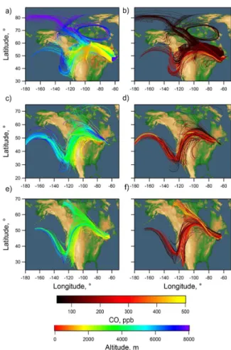
HYSPLIT back trajectories suggest that the plumes en-countered during B621 to B624 originated 2 to 4 days pre-viously, from fires in western Ontario (Fig. 6). Figure 7b and c show how the trajectories were used to identify the source of the fire; Fig. 7b shows 5-day back trajectories with endpoints co-located with the FAAM BAe-146 for the
en-Fig. 6.Five-day HYSPLIT back trajectories whose endpoints
co-locate with every minute of the FAAM BAe-146 flight track, for the whole of the flights B621(a, b), B622(c, d)and B623(e, f). Panels(a), (c)and(e)have been colour-coded by altitude, while
(b), (d)and(f)have been colour-coded by the CO measurement on
the FAAM BAe-146 at the endpoint of each trajectory.
tire flight. When the trajectories are selected that are associ-ated with the enhanced CO and HCN (Fig. 7c), the majority overpass a region in northwestern Ontario that is identified as having had active fires as observed by MODIS. We ac-knowledge that HYSPLIT trajectories are not able to sim-ulate the added buoyancy of a fire plume (pyroconvection); therefore the plume injection profile near to the fires is not known, and as a consequence these air masses may have po-tentially been influenced from further afield such as northern Alberta and the Northwest Territories, for B621 and B623 in particular (Fig. 6). However, Parrington et al. (2013) de-termined a similar age for these plumes by comparing ratios of VOCs to estimate the degree of photochemical processing that the plumes had experienced and hence an approximate age.
0.8
0.6
0.4
0.2
0.0
19:00 21/07/2011
20:00 21:00
GMT 1000
0
HCN, ppt
250 100
CO, ppb
1900 1850
CH
4, ppb
390 380
CO
2
, ppm
3000 2000
Altitude, m
80
70
60
50
40
30
20
Latitude, °
-140 -120 -100 -80 -60 Longitude, °
60
50
40
30
Latitude, °
-120 -100 -80 -60 Longitude, °
4000
3000
2000
1000
0
Altiutude, m
350
340
330
320
310
Brightness temperature, K
a)
b)
c)
Fig. 7. (a)Time series whilst sampling a biomass burning plume
near the coast of Newfoundland during flight B624. The red back-ground indicates that the sampling was in a BB plume.(b) HYS-PLIT 5-day back trajectories for the whole of flight B624. The tra-jectories were started at 60s intervals along the flight starting point. (c)Only the back trajectories that end whilst flying in a biomass burning plume, as identified by the in situ HCN and CO measure-ments on the FAAM BAe-146. Markers are active fires detected by MODIS for the 5 days prior to the flight.
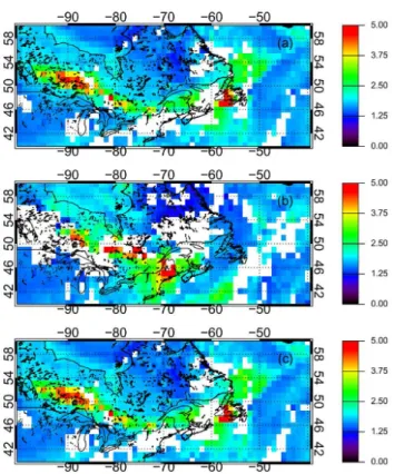
air masses that were associated with BB passed over the same fire region in northwestern Ontario as indicated by the HYS-PLIT trajectories (Figs. 6 and 7). Column-integrated sensitiv-ity plots, from NAME, for flights B622 and B623 are shown in Fig. 8. However, when examining only the surface foot-print over the 5-day air mass history (see the bottom panels of Fig. 8), we see a mixed picture. For B622 (Fig. 8d), there is a footprint in close proximity to the fires detected by MODIS (relative sensitivity to northern Ontario fires=1.9 %). How-ever, for B623 (Fig. 8b), there is little evident surface contact over the 5-day history in regions with significant fire activity (relative sensitivity to northern Ontario fires=0.1 %). This nicely illustrates the efficacy and pitfalls of air mass history analysis using Lagrangian trajectory and dispersion models run backwards in time. For B622, NAME guides us well in the surface attribution of BB sources, while for B623, if we were not otherwise expectant of dynamics such as active
py-Fig. 8.NAME total column (aandc) and surface (bandd)
sensi-tivity footprints for two BB plumes sampled during flight B623 (a andb) and B622 (candd). Darker shading represents a greater sen-sitivity to that region. Markers are active fires detected by MODIS for the 5 days prior to the flight, and they are coloured by the fire radiative power (FRP).
roconvection (Gonzi and Palmer, 2010; Glatthor et al., 2013), then NAME would suggest a non-combustion surface source. The fact that all trajectories (both HYSPLIT and NAME) pass over the fire region is consistent with the injection of material into those higher-level trajectories by pyroconvenc-tion, which is known to be active in the area. Without prior knowledge of the injection profile of material it is not possi-ble to accurately model dispersion in the forward frame, yet these dynamical history fields from NAME and HYSPLIT together nicely illustrate the passage of air over the fire re-gion.
Fig. 9.The daytime mean total column CO (1×10¹⁸mol cm−2)
on a 1◦ by 1◦ grid from the Infrared Atmospheric Sounding Interferometer (IASI) on the MetOp-A satellite for the dates (a)18 July 2011,(b)20 July 2011 and(c)21 July 2011.
IASI total column (TC) CO (daytime overpass) values, re-trieved using the FORLI algorithm (Kerzenmacher et al., 2012) (Fig. 9), are visually compared here to the FAAM BAe-146 CO in situ concentrations, to provide further illus-tration that the enhanced concenillus-trations of CO came from in-plume sampling. IASI shows enhancements in approxi-mately the same location as those identified by the FAAM BAe-146. It is also able to show that the plume covers much of the eastern Canadian coast. The satellite measurements also support the suggestion that the plumes originated from fires in northwestern Ontario.
In theory, as long as the atmospheric lifetime of a species is significantly longer than the age of a plume, it should be possible to calculate ER using measurements in plumes that are several days old, since the calculated NEMR should be approximately equal to the ER at source. However, due to the strong vertical gradients in CO2 and CH4 (Fig. 2) that
were observed over Canada, further consideration needs to made before NEMRs can be calculated for plumes that have been lofted out of the boundary layer into the free tropo-sphere. When a plume is sampled at several altitudes it can be expected that it may have mixed with background air with composition reflecting different origins. As a result when the profile is examined as a whole, strong correlation between
two pyrogenic species may not be observed and the uncer-tainty in the calculation of a NEMR would be large. This lack of correlation may also be due to several different ERs at source that mix during transport to the receptor site.
When the individual flights were analysed as a whole cor-relations between CO, CH4and CO2 were in general weak
(R2< 0.4). This was still the case when filters for BB were applied using HCN or CH3CN. For this reason, it is
nec-essary to partition the flights into individual constant alti-tude runs or vertical profiles to calculate NEMRs. In general, correlation was found to be more robust when the individ-ual runs are examined separately. Table 2 shows NEMRs for all runs and profiles when the correlation coefficient (R2)is greater than 0.60. Where possible EFs are also calculated as-suming no chemical loss during transport.
The calculated CH4 EFs range between 1.8±0.2 and
6.1±1 g (kg dry matter)−1, all of which are lower than the
8.5 g (kg dry matter)−1that was determined when the
north-western Ontario fires were sampled in the near field. How-ever, as mentioned in Sect. 3.1, the aged plumes originated from a period of younger fires and more intense activity. Such fires would typically have a higher MCE (Wooster et al., 2011), which is representative of a larger proportion of flam-ing combustion and therefore a lower proportion of reduced compounds, such as CH4. This highlights the difficulty in
calculating budgets for BB, since fires in one region with ap-proximately the same vegetation type can have such a range of EFs.
For all CH4 EFs we find a regression slope of EF = −47×MCE+47 (R2=0.54). A similar relationship was found by several previous studies, such as Yokel-son et al. (2008) for fires in a tropical forest (EF
= −47×MCE+49, R2=0.72), Yokelson et al. (2003) for savanna fires (EF= −49×MCE+48, R2=0.86) and Korontzi et al. (2003) also for savannah fires (EF= −48×MCE+47, R2=0.88). However, van Leeuwen and van der Werf (2011), who synthesised literature values, found a steeper relationship for extra-tropical forests (EF= −59.992×MCE+60.967) though with weaker correlation (R2=0.27).
1200
1000
800
600
400
200
0
HCN, ppt
400 350 300 250 200 150 100 50
CO, ppb R2= 0.94
1900
1890
1880
1870
1860
1850
1840
CH
4
, ppb
300 200
100
CO, ppb
12
10
8
6
4
2
0
Time airmass spent over HBL below 1000m, Hours
50
40
30
20
10
0
Time airmass spent over HBL below 2000m, Hours
All R2= 0.70
Airmasses that overpass HBL R2= 0.94 y= 0.170x+1841
a)
b)
Fig. 10.Tracer–tracer relationships for a BB plume sampled during
flight B624. Plot(b), showing the relationship between CH4 and CO, has been colour-coded and sized according to the length of time the HYSPLIT trajectories spent over wetlands near Hudson Bay (HBL).
strong agreement is seen for hydrocarbons such as C2H6
(R2=0.97) and C3H8(Propane,R2=0.88).
The BB plume is not as clearly defined in the CH4 and
CO2time series as it is for the other species associated with
biomass burning. This is expected to be partly due to their proportionately higher mean background relative to their typ-ical enhancement and also because there are additional non-BB sources and sinks of these gases relative to CO and HCN (e.g. biospheric uptake and wetland biogenic emission). Cor-relation between CO2 and CO is very weak (R2=0.03).
This suggests that the majority of the BB CO2signal for this
plume has been removed during transport due to a combina-tion of biospheric uptake and mixing with other air masses.
However, even though the correlation between CH4 and
CO is still strong (R2=0.70), a single mixing line cannot be identified in the scatter plot with CO (Fig. 10b) when using the threshold criterion used in the near-field analysis
earlier. This suggests that there may have been mixing into the plume by a localised source during trajectory from fire source to sampling location. Back trajectories illustrate this diversity. We see that during the flight a variety of air masses were sampled, including some that had recently descended from the free troposphere (> 4 km) over the Arctic in the po-lar jetstream. As expected, these air masses are associated with the lowest amounts of CO, typically less than 100 ppb. Other trajectories have originated from the southern US.
The trajectories suggest that since being emitted the plume has travelled over central Canada before being sampled. Dur-ing this time it is likely that the plume will have mixed with air masses containing enhanced CH4 from biogenic
emis-sions associated with the Canadian wetlands, e.g. the Hud-son Bay Lowlands (HBL). This is well known to be a signifi-cant source of CH4and is thought to comprise approximately
10 % of the global boreal wetland emissions of CH4, or about
2.3 Tg per year (Pickett-Heaps et al., 2011). To investigate this further we define the HBL as the geographic region 50– 60◦N, 75–96◦W. Figure 10b colour-codes the scatter plot ac-cording to the length of time that the trajectories spent in this region below 2000 m, and the markers have also been sized depending on the length of time the trajectories spent within this region below 1000 m. The longer an air mass spends at low altitude within this region, the more sensitive it will be to HBL as a source of CH4. An NEMR of 0.170±0.003
(R2=0.97) can be calculated for just those air masses that have passed over HBL below 1000 m. Though not unrealis-tic, this is larger than typically measured for BB, suggesting that the enhancement may not be purely due to BB. As a gen-eral point, we report NEMRs for aged plumes with the im-portant caveat that the impacts (and therefore uncertainty) of mixing cannot be quantified using the available dataset. This is an important consideration for existing and future datasets of this type where far-field NEMRs have been calculated and careful analysis of multiple tracers and air mass history must always accompany any such attempt.
A clear region where CH4is anti-correlated with both CO2
(R2=0.74) and CO (R2=0.55) can be identified (Fig. 10b), with enhancement ratios of (−3.79±0.04)×10−3mol CH4
(mol CO2)−1and−0.284±0.003 mol CH4(mol CO)−1. This
could suggest mixing or advection of an aged fire plume into a region of an enhanced CH4 surface flux (e.g.
bio-genic emission of CH4over wetlands as noted in the
results in the calculated NEMR plume no longer being rep-resentative of the fire ER (Mauzerall et al., 1998; Crounse et al., 2009; Yokelson et al., 2013).
5 Conclusions
Airborne in situ measurements of CO2, CH4and other trace
gases were made over eastern Canada, using the FAAM BAe-146 research aircraft, as part of the BORTAS exper-iment. Both CO2 and CH4 showed a wide degree of
vari-ability, which ranged 371.5 to 397.1 ppm for CO2, and 1797
to 1968 ppb for CH4, representing the unique nature of the
various fire plumes sampled. Vertical concentration profiles were found to be broadly comparable with previous measure-ments, such as those from the ARCTAS project and reanal-ysed composition fields, that assimilate IASI/MOPITT satel-lite measurements, from the European Union funded MACC project. Source-specific tracers were used to distinguish be-tween air masses. CO2 extrema were characterised by BB
emissions and biospheric uptake, while CH4concentrations
were dominated by both BB and biogenic emissions. BB plumes were sampled throughout the troposphere over an altitude range of ∼900 m to ∼8000 m. Near-field sampling of fires in northwestern Ontario yielded EFs of 1512±185 g (kg dry matter)−1 and 8.5±0.9 g (kg dry matter)−1for CO2 and CH4, respectively. Using a
combination of in situ HCN measurements, Lagrangian tra-jectory models and MODIS active fire maps, it was found that plumes from this region were sampled several thousand kilometres downwind when they were 2 to 4 days old. It was found that significant uncertainties exist when calculat-ing EF/ERs from measurements in aged plumes due to the mixing that can occur with non-fire sources during trans-port such as biogenic emissions in this case and that special care must be taken when interpreting far-field data of this type in both existing and future BB datasets. In these aged plumes, EFs were found to vary between 1618±216 and 1702±173 g (kg dry matter)−1 of CO2 and 1.8±0.2 and
6.1±1 g (kg dry matter)−1of CH4. In summary, the results
from this study provide a novel set of fire emission factors and climatological statistics that will inform modelling and process-related studies in the Canadian boreal region.
Acknowledgements. The authors wish to thank all those involved in the BORTAS project. Airborne data were obtained using the FAAM BAe-146 Atmospheric Research Aircraft (ARA) operated by Directflight Ltd (DFL) and managed by the Facility for Airborne Atmospheric Measurements (FAAM), which is a joint entity of the Natural Environment Research Council (NERC) and the UK Meteorological Office. MACC Data provided by the MACC-II project, funded by the European Union under the 7th Framework Programme. The authors would like to thank A. Agusti-Panareda and S. Massart (ECMWF) for advice about the use of the MACC dataset. IASI CO data provided by LATMOS/CNRS & ULB. The authors are grateful to Doug Worthy (Environment Canada) for
providing CO2 and CH4 data from the Sable Island monitoring station. The ABLE 3B 10 s merges were obtained from the NASA Global Tropospheric Experiment data archive at the LaRC DACC. S. J. O’Shea is in receipt of a NERC PhD studentship. This research was supported by the Natural Environment Research Council under grant number NE/F017391/1.
Edited by: S. Matthiesen
References
Akagi, S. K., Yokelson, R. J., Wiedinmyer, C., Alvarado, M. J., Reid, J. S., Karl, T., Crounse, J. D., and Wennberg, P. O.: Emis-sion factors for open and domestic biomass burning for use in atmospheric models, Atmos. Chem. Phys., 11, 4039–4072, doi:10.5194/acp-11-4039-2011, 2011.
Akagi, S. K., Craven, J. S., Taylor, J. W., McMeeking, G. R., Yokel-son, R. J., Burling, I. R., Urbanski, S. P., Wold, C. E., Seinfeld, J. H., Coe, H., Alvarado, M. J., and Weise, D. R.: Evolution of trace gases and particles emitted by a chaparral fire in California, Atmos. Chem. Phys., 12, 1397–1421, doi:10.5194/acp-12-1397-2012, 2012.
Andreae, M. O., and Merlet, P.: Emission of trace gases and aerosols from biomass burning, Global Biogeochem. Cy., 15, 955–966, doi:10.1029/2000gb001382, 2001.
Benedictow, A., Blechschmidt, A.-M., Bouarar, I., Cuevas, E., Clark, H., Flentje, H., Griesfeller, J., Huijnen, V., Huneeus, N., Jones, L., Kapsomenakis, J., Kinne, S., Lefever, K., Razinger, M., Richter, A., Schulz, M., Thomas, W., Thouret, V., Vrekous-sis, M., Wagner, A., and Zerefos, C.: The MACC reanalysis: An 8-year data set of atmospheric composition, MACC-II De-liverable D_83.4, http://www.gmes-atmosphere.eu/documents/ maccii/deliverables/val/ (last access: 22 May 2013), 2013. Cammas, J.-P., Brioude, J., Chaboureau, J.-P., Duron, J., Mari, C.,
Mascart, P., Nédélec, P., Smit, H., Pätz, H.-W., Volz-Thomas, A., Stohl, A., and Fromm, M.: Injection in the lower strato-sphere of biomass fire emissions followed by long-range trans-port: a MOZAIC case study, Atmos. Chem. Phys., 9, 5829–5846, doi:10.5194/acp-9-5829-2009, 2009.
Chevallier, F., Ciais, P., Conway, T. J., Aalto, T., Anderson, B. E., Bousquet, P., Brunke, E. G., Ciattaglia, L., Esaki, Y., Frohlich, M., Gomez, A., Gomez-Palaez, A. J., Haszpra, L., Krummel, P. B., Langenfelds, R., Leuenberger, M., Machida, T., Maignan, F., Matsueda, H., Morgui, J. A., Mukai, H., Nakazawa, T., Peylin, P., Ramonet, M., Rivier, L., Sawa, Y., Schmidt, M., Steele, P., Vay, S. A., Vermeulen, A. T., Wofsy, S. C., and Worthy, D.: CO2 surface fluxes at grid point scale estimated from a global 21- year reanalysis of atmospheric measurements, J. Geophys. Res., 115, D21307, doi:10.1029/2010JD013887, 2010.
Christian, T. J., Yokelson, R. J., Carvalho, J. A., Jr., Griffith, D. W. T., Alvarado, E. C., Santos, J. C., Neto, T. G. S., Gurgel Veras, C. A., and Hao, W. M.: The tropical forest and fire emissions experiment: Trace gases emitted by smoldering logs and dung from deforestation and pasture fires in Brazil, J. Geophys. Res.-Atmos., 112, D18308, doi:10.1029/2006jd008147, 2007. Crounse, J. D., DeCarlo, P. F., Blake, D. R., Emmons, L. K.,
Cen-tral Mexican Plateau, Atmos. Chem. Phys., 9, 4929–4944, doi:10.5194/acp-9-4929-2009, 2009.
Crutzen, P. J., Heidt, L. E., Krasnec, J. P., Pollock, W. H., and Seiler, W.: Biomass burning as a source of atmospheric gases CO, H2, N2O, NO, CH3CL and COS, Nature, 282, 253–256, doi:10.1038/282253a0, 1979.
Damoah, R., Spichtinger, N., Forster, C., James, P., Mattis, I., Wandinger, U., Beirle, S., Wagner, T., and Stohl, A.: Around the world in 17 days – hemispheric-scale transport of forest fire smoke from Russia in May 2003, Atmos. Chem. Phys., 4, 1311– 1321, doi:10.5194/acp-4-1311-2004, 2004.
Damoah, R., Spichtinger, N., Servranckx, R., Fromm, M., Elo-ranta, E. W., Razenkov, I. A., James, P., Shulski, M., Forster, C., and Stohl, A.: A case study of pyro-convection using transport model and remote sensing data, Atmos. Chem. Phys., 6, 173– 185, doi:10.5194/acp-6-173-2006, 2006.
Davies, T., Cullen, M. J. P., Malcolm, A. J., Mawson, M. H., Stani-forth, A., White, A. A., and Wood, N.: A new dynamical core for the Met Office’s global and regional modeling of the atmosphere, Q. J. Roy. Meteorol. Soc., 608, 1759–1782, 2005.
de Gouw, J. A., Warneke, C., Parrish, D. D., Holloway, J. S., Trainer, M., and Fehsenfeld, F. C.: Emission sources and ocean uptake of acetonitrile (CH3CN) in the atmosphere, J. Geophys. Res.-Atmos., 108, 4329, doi:10.1029/2002jd002897, 2003.
Dlugokencky, E. J., Walter, B. P., Masarie, K. A., Lang, P. M., and Kasischke, E. S.: Measurements of an anomalous global methane increase during 1998, Geophys. Res. Lett., 28, 499–502, doi:10.1029/2000gl012119, 2001.
Dlugokencky, E. J., Nisbet, E. G., Fisher, R., and Lowry, D.: Global atmospheric methane: budget, changes and dangers, P. T. R. Soc. A, 369, 2058–2072, doi:10.1098/rsta.2010.0341, 2011. Draxler, R. R. and Rolph, G. D.: HYSPLIT (HYbrid Single-Particle
Lagrangian Integrated Trajectory) Model, NOAA Air Resources Laboratory, Silver Spring, MD, USA, 2003.
Forster, P. and Ramaswamy, V.: Changes in Atmospheric Con-stituents and in Radiative Forcing, Climate Change 2007: the Physical Science Basis, Cambridge Univ. Press, Cambridge, UK, 129–234, 2007.
Gerbig, C., Schmitgen, S., Kley, D., Volz-Thomas, A., Dewey, K., and Haaks, D.: An improved fast-response vacuum-UV reso-nance fluorescence CO instrument, J. Geophys. Res.-Atmos., 104, 1699–1704, doi:10.1029/1998jd100031, 1999.
Gillett, N. P., Weaver, A. J., Zwiers, F. W., and Flannigan, M. D.: Detecting the effect of climate change on Canadian forest fires, Geophys. Res. Lett., 31, L18211, doi:10.1029/2004gl020876, 2004.
Glatthor, N., Höpfner, M., Semeniuk, K., Lupu, A., Palmer, P. I., McConnell, J. C., Kaminski, J. W., von Clarmann, T., Stiller, G. P., Funke, B., Kellmann, S., Linden, A., and Wiegele, A.: The Australian bushfires of February 2009: MIPAS observations and GEM-AQ model results, Atmos. Chem. Phys., 13, 1637–1658, doi:10.5194/acp-13-1637-2013, 2013.
Gonzi, S. and P. I. Palmer.: Vertical transport of surface fire emis-sions observed from space, J. Geophys. Res., 115, D02306, doi:10.1029/2009JD012053, 2010.
Guenther, A., Karl, T., Harley, P., Wiedinmyer, C., Palmer, P. I., and Geron, C.: Estimates of global terrestrial isoprene emissions using MEGAN (Model of Emissions of Gases and Aerosols from
Nature), Atmos. Chem. Phys., 6, 3181–3210, doi:10.5194/acp-6-3181-2006, 2006.
Harriss, R. C., Wofsy, S. C., Hoell Jr., J. M., Bendura, R. J., Drewry, J. W., McNeal, R. J., Pierce, D., Rabine, V., and Snell, R. L.: The arctic boundary layer expedition (ABLE 3B): July–August 1990, J. Geophys. Res., 99, 1635–1643, 1994.
Hecobian, A., Liu, Z., Hennigan, C. J., Huey, L. G., Jimenez, J. L., Cubison, M. J., Vay, S., Diskin, G. S., Sachse, G. W., Wisthaler, A., Mikoviny, T., Weinheimer, A. J., Liao, J., Knapp, D. J., Wennberg, P. O., Kürten, A., Crounse, J. D., Clair, J. St., Wang, Y., and Weber, R. J.: Comparison of chemical character-istics of 495 biomass burning plumes intercepted by the NASA DC-8 aircraft during the ARCTAS/CARB-2008 field campaign, Atmos. Chem. Phys., 11, 13325–13337, doi:10.5194/acp-11-13325-2011, 2011.
Hilton, F., Armante, R., August, T., Barnet, C., Bouchard, A., Camy-Peyret, C., Capelle, V., Clarisse, L., Clerbaux, C., Co-heur, P.-., Collard, A., Crevoisier, C., Dufour, G., Edwards, D., Faijan, F., Fourrié, N., Gambacorta, A., Goldberg, M., Guidard, V., Hurtmans, D., Illingworth, S., Jacquinet-Husson, N., Kerzen-macher, T., Klaes, D., Lavanant, L., Masiello, G., Matricardi, M., McNally, A., Newman, S., Pavelin, E., Payan, S., Péquignot, E., Peyridieu, S., Phulpin, T., Remedios, J., Schlüssel, P., Serio, C., Strow, L., Stubenrauch, C., Taylor, J., Tobin, D., Wolf, W. & Zhou, D.: Hyperspectral earth observation from IASI, B. Am. Meteorol. Soc., 93, 347–370, 2012.
Hornbrook, R. S., Blake, D. R., Diskin, G. S., Fried, A., Fuelberg, H. E., Meinardi, S., Mikoviny, T., Richter, D., Sachse, G. W., Vay, S. A., Walega, J., Weibring, P., Weinheimer, A. J., Wiedin-myer, C., Wisthaler, A., Hills, A., Riemer, D. D., and Apel, E. C.: Observations of nonmethane organic compounds during ARC-TAS - Part 1: Biomass burning emissions and plume enhance-ments, Atmos. Chem. Phys., 11, 11103–11130, doi:10.5194/acp-11-11103-2011, 2011.
Inness, A., Baier, F., Benedetti, A., Bouarar, I., Chabrillat, S., Clark, H., Clerbaux, C., Coheur, P., Engelen, R. J., Errera, Q., Flem-ming, J., George, M., Granier, C., Hadji-Lazaro, J., Huijnen, V., Hurtmans, D., Jones, L., Kaiser, J. W., Kapsomenakis, J., Lefever, K., Leitão, J., Razinger, M., Richter, A., Schultz, M. G., Simmons, A. J., Suttie, M., Stein, O., Thépaut, J.-N., Thouret, V., Vrekoussis, M., Zerefos, C., and the MACC team: The MACC reanalysis: an 8 yr data set of atmospheric composition, Atmos. Chem. Phys., 13, 4073–4109, doi:10.5194/acp-13-4073-2013, 2013.
Jacob, D. J., Crawford, J. H., Maring, H., Clarke, A. D., Dibb, J. E., Emmons, L. K., Ferrare, R. A., Hostetler, C. A., Russell, P. B., Singh, H. B., Thompson, A. M., Shaw, G. E., McCauley, E., Ped-erson, J. R., and Fisher, J. A.: The Arctic Research of the Compo-sition of the Troposphere from Aircraft and Satellites (ARCTAS) mission: design, execution, and first results, Atmos. Chem. Phys., 10, 5191–5212, doi:10.5194/acp-10-5191-2010, 2010.
Jaffe, D. A. and Wigder, N. L.: Ozone production from wildfires: A critical review, Atmos. Environ., 51, 1–10, doi:10.1016/j.atmosenv.2011.11.063, 2012.