An automated gas exchange tank for determining gas transfer velocities in natural seawater samples

(1)

OSD

11, 693–733, 2014

An automated gas exchange tank for natural seawater

samples

K. Schneider-Zapp et al.

Title Page

Abstract Introduction

Conclusions References

Tables Figures

◭ ◮

Back Close

Full Screen / Esc

Printer-friendly Version Interactive Discussion

Discussion

P

a

per

|

D

iscussion

P

a

per

|

Discussion

P

a

per

|

Discuss

ion

P

a

per

|

Ocean Sci. Discuss., 11, 693–733, 2014 www.ocean-sci-discuss.net/11/693/2014/ doi:10.5194/osd-11-693-2014

Open Access

Ocean Science

Discussions

This discussion paper is/has been under review for the journal Ocean Science (OS). Please refer to the corresponding final paper in OS if available.

An automated gas exchange tank for

determining gas transfer velocities in

natural seawater samples

K. Schneider-Zapp1, M. E. Salter2, and R. C. Upstill-Goddard1

1

Ocean Research Group, School of Marine Science and Technology, Newcastle University, Newcastle upon Tyne, UK

2

Department of Applied Environmental Science, Stockholm University, Stockholm, Sweden

Received: 10 January 2014 – Accepted: 24 January 2014 – Published: 21 February 2014

Correspondence to: K. Schneider-Zapp (klaus.schneider-zapp@ncl.ac.uk)

(2)

OSD

11, 693–733, 2014

samples

Title Page

Tables Figures

◭ ◮

Back Close

Full Screen / Esc

Discussion

P

a

per

|

D

iscussion

P

a

per

|

Discussion

P

a

per

|

Discuss

ion

P

a

per

|

Abstract

In order to advance understanding of the role of seawater surfactants in the air–sea exchange of climatically active trace gases via suppression of the gas transfer veloc-ity (kw), we constructed a fully automated, closed air-water gas exchange tank and

coupled analytical system. The system allows water-side turbulence in the tank to

5

be precisely controlled with an electronically operated baﬄe. Two coupled gas chro-matographs and an integral equilibrator, connected to the tank in a continuous gas-tight system, allow temporal changes in the partial pressures of SF6, CH4 and N2O to be

measured simultaneously in the tank water and headspace at multiple turbulence set-tings, during a typical experimental run of 3.25 h. PC software developed by the authors

10

controls all operations and data acquisition, enabling the optimisation of experimental conditions with high reproducibility. The use of three gases allows three independent estimates ofkwfor each turbulence setting; these values are subsequently normalised

to a constant Schmidt number for direct comparison. The normalised kw estimates

show close agreement. Repeated experiments with MilliQ water demonstrate a typical

15

measurement accuracy of 4 % for kw. Experiments with natural seawater show that

the system clearly resolves the eﬀects onkw of spatial and temporal trends in natural

surfactant activity. The system is an eﬀective tool with which to probe the relationships betweenkw, surfactant activity and biogeochemical indices of primary productivity, and

should assist in providing valuable new insights into the air–sea gas exchange

pro-20

cess.

1 Introduction

Air–sea gas exchange is a critical global process, providing the fundamental link be-tween reactive trace gas production and consumption in the oceans and global at-mospheric processes. For example, the oceans are the largest single sink for

tro-25

(3)

OSD

11, 693–733, 2014

samples

Title Page

Tables Figures

◭ ◮

Back Close

Full Screen / Esc

Discussion

P

a

per

|

D

iscussion

P

a

per

|

Discussion

P

a

per

|

Discuss

ion

P

a

per

|

of tropospheric nitrous oxide (N₂O) (IPCC, 2007) and make significant contributions to the global biogeochemical budgets of several other climate-active gases including methane (CH4), carbon monoxide (CO), dimethyl sulphide (CH3SCH3) and some other

sulphur gases, and a range of halocarbons and hydrocarbons (Upstill-Goddard, 2011). Understanding the physical and biogeochemical controls of air–sea gas exchange is

5

therefore necessary for establishing biogeochemical models for predicting regional and global scale trace gas fluxes and feedbacks.

For a sparingly soluble gas, which applies to almost all gases of global biogeochemi-cal interest, the fluxF (e.g. mol m−2d−1) across the air–sea interface can be considered as a diﬀusion-limited process in a typically 20 µm to 200 µm thick “diﬀusive sub-layer”

10

on the water-side of the interface (Jähne, 2009). It can be written as the product of the driving force, i.e. its concentration diﬀerence between airCa and sea water Cw (e. g.

mol m−3), and the air–sea gas transfer velocityk_w(e. g. cm h−1):

F =_k_w₍_αC_a₋_C_w_{) ,} ₍₁₎

15

whereα is the Ostwald solubility coeﬃcient. Similar equations apply to the exchange of heat and momentum. The concentration diﬀerence term (αCa−Cw) can be directly

measured quite routinely butkwcannot. Moreover, the magnitude ofkwvaries with the

degree of near-surface turbulence; increasing turbulence reduces the depth of the diﬀ u-sive sub-layer, resulting in an increase inkw. Indirect approaches are therefore required 20

to estimatekw in-situ and evaluate its variability in response to environmental forcing

functions generating turbulence. One often used method for in-situ measurement is the so-called “dual tracer technique”, which measures the relative rates of evasion to air of two purposefully released, inert volatile tracers: sulphur hexafluoride (SF6) and

helium-3 (3He). Temporal changes in the ratio of their seawater concentrations, typically

25

measured over 24 h to 48 h time intervals, are used to derivekw estimates which are

then scaled to corresponding values for CO2and other reactive trace gases of interest,

(4)

OSD

11, 693–733, 2014

samples

Title Page

Tables Figures

◭ ◮

Back Close

Full Screen / Esc

Discussion

P

a

per

|

D

iscussion

P

a

per

|

Discussion

P

a

per

|

Discuss

ion

P

a

per

|

time-consuming, logistically complex and expensive, and it provides little, if any, infor-mation on the spatio-temporal variability ofkw. Moreover, when the dual tracerkwdata

are plotted against wind speed as the primary driver of turbulence they show a high degree of scatter. Indeed, uncertainty overkw variability presents one of the greatest

challenges to quantifying the net global air–sea exchange of CO2 (Takahashi et al., 5

2009). While a recent analysis shows that around one half of this uncertainty may be ascribed to experimental and measurement errors inherent in the dual tracer technique (Asher, 2009), this still leaves significantkwvariability unaccounted for. This remaining

variability reflects other environmental forcing functions in addition to wind speed, in-cluding wind fetch, atmospheric stability, sea state, wave breaking, white capping and

10

bubble bursting, sea surface temperature, rain, and the presence of surfactants and other organics (Upstill-Goddard, 2006, 2011).

Surfactants are well known to greatly suppresskwand consequently the rate of air–

sea gas exchange, mostly by modifying sea surface hydrodynamics and hence turbu-lent energy transfer, but also by forming a monolayer physical barrier (McKenna and

15

McGillis, 2004). Natural surfactants are ubiquitous in seawater, being primarily phyto-plankton exudates such as polysaccharides, proteins and lipids, and their degradation products (Gašparović, 2012; Zutić et al., 1981), with additional sources via terrestrial inputs of humic and fulvic acids to coastal waters. Spatio-temporal distributions are therefore highly variable. Surfactants tend to be enriched in the diﬀusive sub-layer

rel-20

ative to underlying water up to high wind speeds (Wurl et al., 2011) but their precise eﬀects onkware not well characterised, studies with natural seawaters being

compar-atively scarce. Most data have been derived using wind flumes and/or open exchange tanks in the laboratory (e.g. Goldman et al., 1988; Frew, 1997; Bock et al., 1999); this in part reflects the specialised nature of the analyses and a need to simplify

exper-25

(5)

OSD

11, 693–733, 2014

samples

Title Page

Tables Figures

◭ ◮

Back Close

Full Screen / Esc

Discussion

P

a

per

|

D

iscussion

P

a

per

|

Discussion

P

a

per

|

Discuss

ion

P

a

per

|

during field experiments. This makes recourse to laboratory based experiments in-escapable.

In order to make further progress in this regard, we have devised a laboratory pro-cedure that enables us to directly evaluate the contrast in kw between natural

sea-waters of varying surfactant content under controlled and reproducible conditions of

5

turbulence. To simplify the system, we generate water-side turbulence, allowing us to concentrate on the important aspects of comparativek_wmeasurements at constant tur-bulence and avoiding unnecessary complication of the system. This simplifies process-understanding and also overcomes diﬃculties associated with simulating wind-induced turbulence in a laboratory. Even though the absolutek_wvalues may not be strictly

com-10

parable to in-situ conditions, this simplification is wholly adequate to achieve our goal of comparativekw measurements at constant turbulence, and is an important step in

understanding more completely the relationships between surfactants, turbulence and

kw. Once this is established, more elaborate experiments in wind-wave facilities can

provide valuable supplementary information.

15

Our system uses a sealed laboratory gas exchange tank with integral water equili-brator. The partial pressures of experimental gases (SF₆, CH₄ and N₂O) in the water and air phases of the system are measured using gas chromatography. Turbulence in the tank can be routinely selected and modified such that inter-sample diﬀerences in

kwexclusively reflect diﬀerences in sample surfactant content, something that cannot 20

currently be achieved through field experiments.

2 System design

2.1 Prior considerations

We previously used a sealed gas exchange tank for examining the microbial controls of air–sea gas transfer (Upstill-Goddard et al., 2003). This featured semi-automated

25

(6)

OSD

11, 693–733, 2014

samples

Title Page

Tables Figures

◭ ◮

Back Close

Full Screen / Esc

Discussion

P

a

per

|

D

iscussion

P

a

per

|

Discussion

P

a

per

|

Discuss

ion

P

a

per

|

required manual operation and large sample volumes, necessitating large and cumula-tive volume corrections, and turbulence control was comparacumula-tively rudimentary. Analyt-ical uncertainty was therefore high but experimental reproducibility and accuracy were not rigorously assessed. Overall system reliability was also rather variable. To ade-quately resolve inter-sample diﬀerences in k_w due to variability in surfactant content

5

demands a redesigned system with vastly improved performance and flexibility. An im-portant aspect of the system described here is its full automation. PC control software developed by the authors controls all operations and data acquisition. This is a key aspect of the system because it guarantees that all experiments are run under identi-cal conditions, free of operator induced variability. It also facilitates the optimisation of

10

experimental run times, which is critical for surfactant focused work because it is es-sential to preserve sample integrity when several samples have been collected along lateral seawater transects for example. Natural surfactants can degrade rapidly and significantly on storage. Such changes are variable and can be diﬃcult to predict due to diﬀerences in organic composition between water samples (Schneider-Zapp et al.,

15

2013). Consequently, when sample storage is unavoidable it should be minimised as far as is practically possible.

2.2 Selection of experimental gases

The use of SF₆, CH₄ and N₂O in the gas exchange experiments is based on our prior experience with them, in particular their ease of analysis, but most importantly because

20

of their relevance in the context of air–sea gas exchange and global biogeochemistry. SF₆is inert and is essentially all man-made, although there is a small geological source (Harnisch and Eisenhauer, 1998), and it is routinely used for estimating kw in-situ

(Wanninkhof et al., 1993; Wanninkhof et al., 1997; Watson et al., 1991; Nightingale et al., 2000). CH₄ and N₂O both have significant marine sources and sinks, are

infra-25

red active and have long atmospheric lifetimes (IPCC, 2007). N2O is also involved

in stratospheric O3 regulation via NOx generation (Nevison and Holland, 1997) and

(7)

OSD

11, 693–733, 2014

samples

Title Page

Tables Figures

◭ ◮

Back Close

Full Screen / Esc

Discussion

P

a

per

|

D

iscussion

P

a

per

|

Discussion

P

a

per

|

Discuss

ion

P

a

per

|

of tropospheric OH and O₃ (Crutzen and Zimmermann, 1991). Both gases are cur-rently increasing in the troposphere, but at variable rates that are not well understood (Dlugokencky et al., 1998, 2001; Khalil, 1993; Prinn et al., 1990; Rigby et al., 2008). Quantifying the constraints on their air–sea exchange rates is therefore critical.

2.3 System overview 5

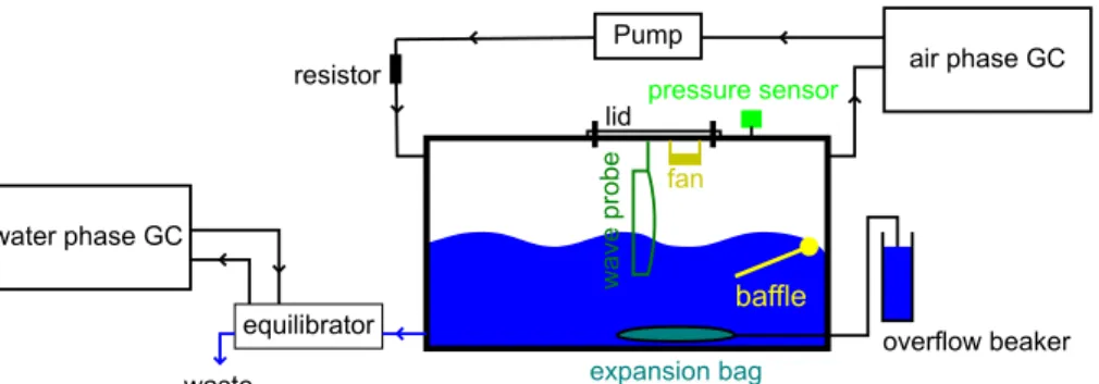
A schematic of the gas exchange system is shown in Fig. 1. Its principal components are: (i) a sealed acrylic gas exchange tank that can be approximately half filled with seawater (Fig. 2 details its major features); (ii) an equilibration system used in prepar-ing tank water subsamples for analysis; (iii) two gas chromatographs (GC’s) identically configured for the analysis of SF6, CH4and N2O, in the tank headspace and in air that 10

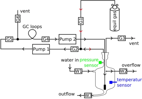
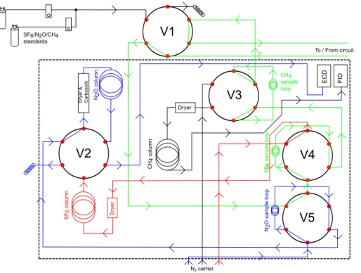
has been equilibrated with a tank water subsample. These components form a contin-uous, sealed circuit that can be decoupled and reconnected as required via the opera-tion of solenoids. Details of the components are given in Sect. 3. The gas equilibraopera-tion system is shown in Fig. 3 and the GC configuration in Fig. 4.

3 System components 15

3.1 Gas exchange tank

The basic structure of the gas exchange tank (Fig. 2) was custom-built (Bay Plastics Ltd, UK) for ourk_w-surfactant work. Subsequent modifications, principally the installa-tion of mechanical and electronic components (see below), were carried out in-house. The tank has an internal base area of 0.73 m×0.48 m, is 0.48 m in height internally and

20

is constructed from 12 mm acrylic. Stainless steel bulkhead connectors are used for all tank connections. The incorporation of a headspace pressure relief valve precludes system over-pressurisation and subsequent damage to the tank structure in the event of system malfunction. The tank is filled with sample gravimetrically to a notional vol-ume of (93.0±0.1) L, leaving a corresponding notional 74.1 L headspace ((1.11±0.01)L

(8)

OSD

11, 693–733, 2014

samples

Title Page

Tables Figures

◭ ◮

Back Close

Full Screen / Esc

Discussion

P

a

per

|

D

iscussion

P

a

per

|

Discussion

P

a

per

|

Discuss

ion

P

a

per

|

is accounted for by the baffle, expansion bag and holders). This method of filling was selected because it is important to reproduce the sample volume precisely. Small dif-ferences in the fill level can have a large effect on the degree of tank water turbulence, which is selected and controlled using an internal acrylic baffle mounted across the full width of the tank on a transverse shaft. The gravimetric procedure overcomes this

5

problem. A stepper motor (PD2-116-60-SE: Trinamic, Germany) is located outside the tank and connected to the baﬄe shaft via a gas-tight bearing and Viton® seal. The motor is operated via a serial RS232 link and allows precise control of the forward and reverse motion of the baﬄe. The tank air-phase (headspace) is continuously mixed us-ing a low throughput fan (Sanyo Denki 9S1212F4011: RS components, UK) that does

10

not create any detectable water turbulence. The fan is mounted on the inside of a re-movable circular tank lid, along with a wave height gauge (Sect. 3.3). The lid facilitates access for maintenance, for internal tank cleaning and for filling with sample and is sealed using a double Viton®O-ring. Viton®is compatible with gaseous hydrocarbons and its use also precludes SF6 memory eﬀects that may be encountered with some 15

other seal materials (Upstill-Goddard et al., 2003).

During operation (Sect. 4.2) aliquots of the tank water are automatically transferred to the equilibration vessel (Sect. 3.2). In order to prevent a progressive decrease in tank internal pressure due to this procedure, an expandable plastic bag (Supel Inert Film 10 L gas sampling bag, Sigma-Aldrich, UK) inside the tank is connected to a small

20

external water reservoir containing artificial seawater (ASW) of salinity≥45 via a water-tight bulkhead fitting. The density contrast between the ASW and the tank seawater (maximum salinity ≈35) ensures a negative buoyancy that prevents the expandable bag from rising from the bottom of the tank. A secondary, larger ASW reservoir is used to maintain the water level inside the small reservoir at the same level as in the

25

exchange tank using a peristaltic pump; an overflow returns any excess back into the larger reservoir, thereby keeping the water level in the smaller reservoir constant.

Pressure in the tank headspace (Ph) is continuously monitored using a transducer

(9)

OSD

11, 693–733, 2014

samples

Title Page

Tables Figures

◭ ◮

Back Close

Full Screen / Esc

Discussion

P

a

per

|

D

iscussion

P

a

per

|

Discussion

P

a

per

|

Discuss

ion

P

a

per

|

output voltage is converted to a digital signal using a USB-6008 (12 bit) ADC (National Instruments, USA). Temperature in the tank water phase is recorded on an autonomous mini data logger (Minilog 8, Vemco, Canada; accuracy 0.2◦C) that is retrieved for data download at the end of each experiment.

3.2 Equilibration Vessel 5

The analysis of dissolved gases by gas chromatography necessitates either a pre-extraction or equilibration step, followed by the measurement of gas partial pressures in the resulting gas phase and corrections for air and water volumes and gas solubilities (Upstill-Goddard et al., 1996). Extraction techniques often involve pre-concentration procedures which can be complicated and the overall extraction eﬃciency can vary

10

significantly. By contrast, automated gas equilibration has been shown to be highly reproducible (Upstill-Goddard et al., 1996). We therefore incorporated a water-air equi-libration vessel as an integral component of the gas exchange tank apparatus. The equilibration vessel has a total internal volume of 183 cm3and has two principal com-ponents: a glass vessel equilibrator and a removable stainless steel equilibration

man-15

ifold (Fig. 3). The design derives from a system we constructed for the high precision analysis of dissolved gases at sea (Upstill-Goddard et al., 1996). The equilibration manifold comprises three lengths of stainless steel tubing silver-soldered through a ta-pered stainless steel plug machined to seat precisely in the neck of the glass vessel to give a gas-tight seal. Two tubes are cut flush to the base of the plug and a third

20

is connected to a stainless steel aerator frit near the bottom of the glass vessel. The frit is a standard chromatography solvent filter (Thames Restek, UK). The equilibration vessel has three water inlet/outlets (all 4 mm i.d.), each connected via a short length of flexible Tygon® tubing to a solenoid (Burkert 0124 2/2 way for aggressive media, Burkert, Germany; W1-W3 in Fig. 3). A digital temperature sensor (DS18B20+;

resolu-25

(10)

OSD

11, 693–733, 2014

samples

Title Page

Tables Figures

◭ ◮

Back Close

Full Screen / Esc

Discussion

P

a

per

|

D

iscussion

P

a

per

|

Discussion

P

a

per

|

Discuss

ion

P

a

per

|

SF₆, N₂O and CH₄ composition (the “equilibrator gas”) is connected via solenoid G1. The gas is circulated through G2, the GC sample loops and back through the equili-brator frit. Solenoid G3 allows venting of the equiliequili-brator during its filling with seawater via W1. Solenoids G1-G3 are Burkert 6013A 2/2 way (Burkert, Germany).

Prior to equilibration the equilibration vessel and all associated GC sample tubing is

5

flushed with the equilibrator gas via solenoid G1. Next the vessel is completely filled with tank water via solenoid W1, all air being displaced via solenoid G3. A headspace of equilibrator gas is then introduced via G1, displacing sample via the overflow and solenoid W2. The fill/displacement cycle is then repeated to ensure the removal of all traces of previous sample and equilibrator gas. The procedure facilitates a reproducible

10

headspace to water volume ratio (Sect. 4.4.2) which is required for accurately correct-ing for solubility-driven phase partitioncorrect-ing durcorrect-ing equilibration (Upstill-Goddard et al., 1996). All solenoids are then closed and G2, G4 and G5 are opened. Two gas sampling pumps (NMP015.1.2KNL: KNF Neuberger AG, Switzerland) circulate the equilibrated sample gas around the closed circuit, through the GC sample loops and back through

15

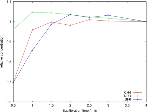
the equilibrating water sample via the aerator frit inside the equilibrator for 4.35 min. Equilbration-time curves (Fig. 5) show that all three gases are fully equilibrated within 3 min. Two pumps are necessary to equalise pressure gradients and thus maintain the internal equilibrator pressure at ambient. Pumping rates are regulated via 8 bit pulse width modulation of the 12 V supply. The speed of pump 1 is kept constant and that of

20

pump 2 is regulated in response to the equilibrator internal pressure.

Following equilibration the pumps are switched oﬀ, all solenoids are closed and G6 is opened for 20 s to allow the GC sample loops to reach ambient atmospheric pressure before injection onto the GC carrier gas lines. This avoids pressure eﬀects that might otherwise interfere with the detector responses.

25

(11)

OSD

11, 693–733, 2014

samples

Title Page

Tables Figures

◭ ◮

Back Close

Full Screen / Esc

Discussion

P

a

per

|

D

iscussion

P

a

per

|

Discussion

P

a

per

|

Discuss

ion

P

a

per

|

than for our experiments with an earlier gas exchange tank (Upstill-Goddard et al., 2003).

Determining equilibration volumes

The relative volumes of water to headspace Va/Vw involved in the equilibration step

must be accurately known in order to facilitate corrections for solubility-driven phase

5

partitioning (Upstill-Goddard et al., 1996). Vw can be determined gravimetrically by

repeatedly generating headspace in the equilibrator. By contrast, system configura-tion precludes directly measuring Va. To overcome this we directly estimated Va/Vw

by equilibration, similar to Upstill-Goddard et al. (1996). The gas exchange tank was filled with 93 L MilliQ water (resistivity typically 18.2 MΩcm−3: Millipore Corporation,

10

USA) enriched with SF₆, N₂O, and CH₄, sealed and equilibrated by operating the baf-fle until the gas partial pressures in both the equilibrator headspace and in the tank headspace remained constant for>12 h. For this measurement ultra high purity (UHP) N₂(>99.999 % N₂, no detectable SF₆, N₂O or CH₄) was used as equilibrator gas, i. e.

C0=0. Concentrations in the tank headspace and equilibrator were then determined 15

multiple times and averaged. These values were used together with the appropriate Ostwald solubilities of SF₆ (Bullister et al., 2002), CH₄ (Wiesenburg and Guinasso, 1979) and N₂O (Weiss and Price, 1980) at the temperature and pressure of equili-bration and the tank headspace and water volumes, to calculate Va/Vw according to

Eq. (17). For the system as currently configuredVa/Vw=0.79±0.02. 20

3.3 Wave height gauge

A capacitance-type high-precision wave height gauge (AWP-24; 30 cm double strand sensing wire, Akamina Technologies, Canada) is used. Analogue output voltage is digi-tised at 400 Hz (USB-6008 ADC, National Instruments, USA). The output voltage of the device is linearly proportional to the water level.

(12)

OSD

11, 693–733, 2014

samples

Title Page

Tables Figures

◭ ◮

Back Close

Full Screen / Esc

Discussion

P

a

per

|

D

iscussion

P

a

per

|

Discussion

P

a

per

|

Discuss

ion

P

a

per

|

The probe is routinely calibrated to determine the relationship between water depth and output voltage by filling the gas exchange tank with sample water and progressively immersing the probe step-wise into the water. This is done by mounting the probe on a rod with precisely machined holes at 1 cm intervals. For each step the rod is bolted through one of the holes to a sturdy mount secured to the tank. After waiting for the

5

water surface to settle, the output voltage is averaged over 10 s. A line is fitted to the immersion depth – voltage relation.

3.4 Ancillary measurements

Absolute pressure (P₀) and temperature (T) in the laboratory are measured using a dig-ital sensor (Sensortec BMP085; pressure range 300–1100 hPa; absolute pressure

ac-10

curacy 1 hPa; absolute temperature accuracy 0.5◦: Bosch, Germany).

3.5 Gas chromatography

The need to determine the partial pressures of SF₆, CH₄and N₂O in both the air and water phases during an experiment precludes using a single GC; this would necessi-tate long sampling intervals and/or a long experimental duration, with consequent loss

15

of experimental resolution. Therefore two identically configured GC’s were used (both HP 5890), one for analysing tank headspace (“air-phase GC”) and one for analysing equilibrator air following water sample equilibration (“water phase GC”). The analysis is identical in each GC, being isothermal (60◦) and based on methods developed in our laboratory (Upstill-Goddard et al., 1990, 1996, 2003). A schematic is shown in

20

Fig. 4. A series of motor-driven stainless steel chromatography valves, V1–V5 in Fig. 4 (Valco: Vici AG, Switzerland), allow the selective switching of tank headspace, equili-brator headspace and calibration standards onto the separating columns (one each for SF6, N2O and CH4 in each GC) and detectors, via fixed volume sample loops

(inter-nal volume: SF6 10 mL, CH4 1 mL, N2O 1.5 mL). Chromatographic separation of SF6 25

(13)

OSD

11, 693–733, 2014

samples

Title Page

Tables Figures

◭ ◮

Back Close

Full Screen / Esc

Discussion

P

a

per

|

D

iscussion

P

a

per

|

Discussion

P

a

per

|

Discuss

ion

P

a

per

|

both separated on 80–100 mesh Porapak Q columns (CH₄, 4 m×1.75 mm i. d.; N₂O, 5 m×1.75 mm i. d.). The GC carrier gas is UHP N2. Flow rates are typically around

25cm3min−1for CH4and N2O, and 50 cm 3

min−1for SF6. Water vapour produced

dur-ing sample equilibration is removed usdur-ing Mg(ClO4)2 and CO2is removed using NaOH

(Upstill-Goddard et al., 1996). Detection of CH₄uses a flame ionization detector (FID)

5

at 300◦whereas detection of N2O and SF6uses an Electron Capture Detector (ECD)

with a63Ni source at 350◦.

The GC responses are integrated automatically using proprietary GC software (Clar-ity: DataApex, Prague, Czech Republic). Method calibration uses a series of mixed calibration standards prepared by pressure dilution in UHP N2 (Upstill-Goddard et al., 10

1990, 1996). Analytical precisions are typically±1 % CH₄,±0.8 % N₂O, and±1 % SF₆. All three gases are analysed in less than 8 min.

3.6 Limits of detection

Minimum detectable levels of SF6, N2O and CH4have been determined by estimating

the detector responses corresponding to a signal to baseline noise ratio of 2 and

di-15

viding by the detector peak width (peak area/peak height) in seconds (Upstill-Goddard et al., 1996). Minimum detectable levels are 0.5 pptv SF6, 0.2 ppbv N2O and 10 ppbv

CH₄. However, in practice the partial pressures of all three gases in the equilibrator gas combined with solubility considerations (Bullister et al., 2002; Wiesenburg and Guinasso, 1979; Weiss and Price, 1980) preclude operating the detectors close to

20

these limits.

4 Experimental procedure

(14)

OSD

11, 693–733, 2014

samples

Title Page

Tables Figures

◭ ◮

Back Close

Full Screen / Esc

Discussion

P

a

per

|

D

iscussion

P

a

per

|

Discussion

P

a

per

|

Discuss

ion

P

a

per

|

4.1 Field sampling

Large volume water samples (≈100 L) for the gas exchange experiments were col-lected during two coastal North Sea transects of R/V Princess Royal, on 4 Octo-ber 2012 and 13 February 2013. On both, samples were collected from 5 fixed locations approximately equally spaced up to 20 km oﬀ-shore of the UK Northumberland coast

5

(Fig. 6). The samples were drawn with an on-board sampling pump and stored on-deck in “aged” polyethylene seawater carboys (i.e. all leachable components removed using concentrated HCl solution). Additional samples for the measurement of surfactant ac-tivity were collected from the surface microlayer (SML) using a Garrett (1965) screen (for further details of our Garrett screen samplers, see Schneider-Zapp et al., 2013)

10

and from the underlying water (ULW) using a stainless steel bucket. After decanting into sterile polypropylene sampling tubes these samples were kept refrigerated in the dark at 4◦ to minimise degradation during pre-analysis storage (Schneider-Zapp et al., 2013). Salinity and temperature were measured using a hand-held probe. Meteorolog-ical data were acquired via an on-board weather station.

15

4.2 Gas exchange experiments

The inside of the gas exchange tank is repeatedly cleaned and filled/rinsed with MilliQ water until surfactant activity (SA) in the tank water surface microlayer (SML) is an-alytically identical to that of fresh MilliQ. The SML is routinely collected with a small Garrett (1965) screen and SA is measured by hanging mercury drop AC voltammetry

20

(see Sect. 4.3).

Following cleaning and thorough rinsing of the inside of the tank with sample, the tank is filled with 93 L of sample (measured gravimetrically), which is added directly from sampling carbuoys using a peristaltic pump. During this procedure 1.1 L of sam-ple is decanted directly from one of the carbuoys into a sealable glass bottle and

en-25

(15)

OSD

11, 693–733, 2014

samples

Title Page

Tables Figures

◭ ◮

Back Close

Full Screen / Esc

Discussion

P

a

per

|

D

iscussion

P

a

per

|

Discussion

P

a

per

|

Discuss

ion

P

a

per

|

grade CH4and 1 cm 3

of 99.998 % research grade N2O are injected into the vessel and

equilibrated with the sample water for 20 min using a small pump and aerator. This gas-enriched subsample is added to the tank at the end of the filling procedure to give the final, notional 93 L volume and the tank is then sealed. The sample volume added to the tank, including that of the gas enriched subsample, is calculated by weighing

5

the carbuoys before, during, and after filling and adjusting for the sample density de-rived from its salinity and temperature. These are measured in the residual sample in the carbuoys directly after filling, using a pre-calibrated hand-held probe, in order to preclude any possible contamination of the tank water sample. The enriched subsam-ple creates a disequilibrium in gas partial pressures between the tank water and tank

10

headspace, so as to drive measureable water-to-air exchange of SF6, N2O and CH4

during the experiment.

A configuration file defining all experimental settings is read by the control program which executes the experiment. The system is optimised to run a gas exchange exper-iment in just under 3.25 h. We routinely use three sequential fixed levels of turbulence,

15

each of 64.5 min duration; corresponding baﬄe frequencies are 0.6 Hz, 0.7 Hz, and 0.75 Hz. GC analysis of the tank headspace and equilibrated water phases is every 10.75 min, enabling 6 measurements of each phase for each selected level of turbu-lence during an experiment. Temperatures and pressures are logged every 0.1 min. Immediately prior to and following each experiment, calibration gas standards are

re-20

peatedly measured on each GC for data calibration and to allow an estimate of detector drift. This is usually less than 2 % over the course of a typical experiment and is cor-rected for by applying a time-dependent linear fit to the detector responses.

Gas concentration uncertainties are estimated using the standard deviation of the standard measurements. For all other measured quantities, specified instrument

accu-25

(16)

OSD

11, 693–733, 2014

samples

Title Page

Tables Figures

◭ ◮

Back Close

Full Screen / Esc

Discussion

P

a

per

|

D

iscussion

P

a

per

|

Discussion

P

a

per

|

Discuss

ion

P

a

per

|

This eﬀect cannot be separated from the statistical error or corrected for, as the drift is irregular.

Estimates of kw are obtained from Eq. (13) using weighted linear regression

(Sect. 4.4.1). The uncertainty is estimated from the weighted fit. Thekwestimates are

then scaled to Schmidt number 660 using Eq. (19) (Sect. 4.4.3). Convention is to scale

5

all measured values ofkw to Schmidt numbers of either 660 or 600, being the values

for CO₂in freshwater and salinity 35 seawater respectively, at 20◦C. Schmidt numbers are obtained from Wanninkhof (1992). From the MilliQ data, a Schmidt number expo-nent ofn=₁_/_{2 was determined using Eq. (20), corresponding to a flat surface. This}

is reasonable, because the baﬄe generated turbulence does not create much surface

10

turbulence (e.g. capillary waves) compared to wind drag (see also the introduction, Sect. 1).

The wave frequency energy spectrum is calculated from the sampled wave height using the method of Welch (1967) (see Harris, 1978, for more information) with a Hann window of length 131 072.

15

4.3 Surfactant measurement

Surfactant activity (SA) is measured using AC voltammetry (Ćosović and Vojvodić, 1982) (Metrohm 797 VA Computrace, Metrohm, Switzerland) with a hanging mercury drop, a silver/silver chloride reference electrode and a platinum wire auxiliary electrode. Samples are brought to salinity 35 prior to measurement by adding surfactant-free NaCl

20

solution. For each measurement, a new mercury drop is created and the first few drops discarded. Surfactants accumulate on the drop atV =₋_{0.6 V for 15 s or 60 s with}

stir-ring (1000 rpm). Alternating voltage scans of 10 mV at 75 Hz produce a current which is measured. Instrument calibration uses the non-ionic soluble surfactant Triton T-X-100. Each response is corrected for the added NaCl solution and expressed as an

25

(17)

OSD

11, 693–733, 2014

samples

Title Page

Tables Figures

◭ ◮

Back Close

Full Screen / Esc

Discussion

P

a

per

|

D

iscussion

P

a

per

|

Discussion

P

a

per

|

Discuss

ion

P

a

per

|

4.4 Theory

4.4.1 Tank gas exchange

For a sealed gas exchange tank containing seawater and air and without gas sources or sinks, Eq. (1) can be used to derive a mass balance:

∂C_a ∂t Va ∂C_w

∂t Vw

!

=_k_w

Cw−αCa

αCa−Cw

A. (2)

5

The solubilityα, volumesVaandVw, and surface areaAare assumed to be constant. In

reality,αdepends on temperature. In practice changes in experimental temperature are of the order of 0.5◦. For such a change in temperature at 20◦, the change inαis<1.6 % for SF₆,<1.4 % for N₂O and<1 % for CH₄ according to published parameterisations

10

(Bullister et al., 2002; Wiesenburg and Guinasso, 1979; Weiss and Price, 1980). Let the height of phasei (i. e. air a or water w) beh_i, i.e.h_i :=V_i/A, and let

D:=Cw−αCa. (3)

For SF₆, which has a very low solubility (Bullister et al., 2002), D≈Cw for all practi-15

cal purposes. In contrast, for CH4and N2O, which are one and two orders of

magni-tude more soluble respectively than SF6(Wiesenburg and Guinasso, 1979; Weiss and

Price, 1980) the value ofCamust be taken account of. Re-arranging Eq. (3), taking the

derivative and using the chain rule results in

∂Ca

∂t =

1

α

_∂C

w

∂t −

∂D ∂t

=kw

ha

D, (4)

(18)

OSD

11, 693–733, 2014

samples

Title Page

Tables Figures

◭ ◮

Back Close

Full Screen / Esc

Discussion

P

a

per

|

D

iscussion

P

a

per

|

Discussion

P

a

per

|

Discuss

ion

P

a

per

|

where Eq. (2) (top) has been used in the last equality. Substituting ∂Cw

∂t into Eq. (2)

(bottom), a diﬀerential equation inDis obtained:

∂D

∂t +kw

1

hw

+ α

ha

| {z }

=_:β

=₀ ₍₅₎

Solving this gives

5

D=_D₀_{exp (}₋_k_w_βt_{) ,} ₍₆₎

whereD0:=D(t=0).

Due to conservation of mass, the total amount of gasN in the system must remain constant. Hence:

10

N=CaVa+CwVw=const. (7)

This relation serves as a routine check of the experimental results and system integrity; a change in the value ofNduring the experiment implies system leaks and/or defective chromatography.

15

At each equilibration step the tank water volumeVwdecreases (here assumed

instan-taneously) by volumeVs, such thatVw>=Vw<−Vs, whereVw<andVw>are the tank water

volumes before and after drawing the sample, respectively. The effect is to change the value of β so that the differential equation no longer has constant coefficients. How-ever, within each interval [t_n,t_n+1] between two measurements at timestnandtn+1, the 20

volumes are constant and Eq. (6) can be used. At each sampling step the values of the coeﬃcients change instantaneously; the variables at the end of the previous interval become the initial conditions for the next interval. IfV_e,n=_nV_s_{is the total water volume}

already extracted attn, using the abbreviationsVw,n:=Vw|t=_t_n,D_n:=D(t=t_n) and

β_n:=β|_t=_t_n= A

Vw,n−1−Vs

+Aα

Va

= A

Vw,0−nVs

+Aα

Va

= 1

hw,0−nhs

+ α

ha

(8)

(19)

OSD

11, 693–733, 2014

samples

Title Page Abstract Introduction Conclusions References Tables Figures ◭ ◮ ◭ ◮ Back Close

Full Screen / Esc

Printer-friendly Version Interactive Discussion Discussion P a per | D iscussion P a per | Discussion P a per | Discuss ion P a per | derives

Dn=Dn−1exp(−kwβn(tn−tn−1)) (9)

The first water sample is drawn att0, the experiment starts running with the reduced

water volumeVw−Vsand thus the system response is 5

Dn=D0exp



−k_w

n

X

j=1

βj(tj−tj−1)



 (10)

Note that forn=_{0, the sum is zero and the equation is identical to the original Eq. (6).}

The new solution Eq. (10) is not in the form exp−kwβt but has a sum of diﬀerenttj in

its exponential. It can be solved forkw; however it diverges forn=0. This is overcome 10

by conversion to the form exp−kwβt as

Dn=D0exp

      

−kw





n

X

j=1

βj

t_j−t_j₋1

tn−t0





| {z }

=_:B_n

(tn−t0)

       (11) with

Bn:=

n

X

j=1

βj

t_j−t_j₋1

t_n−t0

= A

t_n−t0

n

X

j=1

t_j−t_j₋1

Vw,0−jVs

+Aα

Va

. (12)

15

Note that B0=β0 (eqs. 11 and 6). For Vs=0, we obtainBn=β0 and the solution

reduces to Eq. (6) witht0=0. WithVs>0, the value ofBn increases (the denominator

in each summand is decreased) and consequently D decreases progressively more rapidly with increasing experimental run time during which further water is extracted

(20)

OSD

11, 693–733, 2014

samples

Title Page

Tables Figures

◭ ◮

Back Close

Full Screen / Esc

Discussion

P

a

per

|

D

iscussion

P

a

per

|

Discussion

P

a

per

|

Discuss

ion

P

a

per

|

from the tank. Consequently some fraction of the decrease inD is due to volume ex-traction. Without any correction for thiskwis overestimated. The factor

tj−tj−1

t_n−t₀ is applied

as a weight factor for any given water volume during the experiment.

The solution can be expressed in logarithmic form to derive a linear fit obtainingkw

as

5

χ_n:= 1

B_nln

D0

D_n =kw(tn−t0) . (13)

The mass balance Eq. (7) also has to be adjusted to account for the water loss on sampling:

Nn=Vw,nCw,n+

n

X

j=1

Cw,j−1Vs+VaCa,n. (14)

10

4.4.2 Water sample equilibration

We can consider a water sample of volumeVwin the equilibrator with an initial dissolved

gas concentrationCwat in situ pressureP1and temperatureT1. The number of moles

of gas in the water isN1=CwVw. 15

The water sub-sample then equilibrates with a head space of volumeVa and initial

gas concentration C0. The total number of moles of gas in the equilibrator is then N=N1+N0=VwCw+VaC0. During equilibration the gas partitions according toαC

′

a= Cw′, where α is the Ostwald solubility coeﬃcient.N remains constant (conservation of

mass), thus

20

VaCa′ +VwC′w=VaC′a+VwαC′a=VaC0+VwCw. (15)

Solving forCwresults in

Cw=

Va

Vw

(21)

OSD

11, 693–733, 2014

samples

Title Page

Tables Figures

◭ ◮

Back Close

Full Screen / Esc

Discussion

P

a

per

|

D

iscussion

P

a

per

|

Discussion

P

a

per

|

Discuss

ion

P

a

per

|

which can be used to back-calculate the gas concentration in the water sample using

Ca′.

For evaluating Eq. (16), the water–headspace volume ratio Va/Vw is required. It is

determined by a measurement with knownCwand C′aso that Eq. (15) is then solved

forV_a/V_w:

5

Va

Vw

=Cw−αC

′

a

Ca′−C0

. (17)

4.4.3 Schmidt number scaling

The value ofkw for any gas is a function of its Schmidt numberSc, which is defined

as the ratio of the viscosity of water to the corresponding gas diﬀusivity at the requisite

10

temperature, i.e.Sc=_ν/D_{. Theory predicts the scaling}

kw=

u_∗

RSc

−n ₍₁₈₎

where u_∗ is the friction velocity, R is the resistance for momentum transfer and the exponent n is equal to 2/3 for a smooth surface and 1/2 for a rough surface with

15

a smooth transition (Richter and Jähne, 2010). This relation allows the interconversion ofk_wfor any given gas tok_wfor any other specified gas. Given two gases 1 and 2 with transfer velocitieskw1 and kw2 and Schmidt numbers Sc1 and Sc2, respectively, one

obtains

kw1=

_Sc

1

Sc2

−n

kw2. (19)

20

Simultaneous measurements of two gases with diﬀerent Schmidt numbers can be used to calculate the exponent:

n= ln

k_w1 k_w2

lnSc2

Sc1

=ln

k_w1 k_w2

lnD1

D2

(20)

(22)

OSD

11, 693–733, 2014

samples

Title Page

Tables Figures

◭ ◮

Back Close

Full Screen / Esc

Discussion

P

a

per

|

D

iscussion

P

a

per

|

Discussion

P

a

per

|

Discuss

ion

P

a

per

|

4.4.4 Wave spectra

Letη(x,t) be the (vertical) surface displacement from the mean surface level at hori-zontal position x=(x1,x2) and time t. Its mean value is zero, i.e. hηi=0. The higher

moments of the displacement are important for characterising the wave field. The autocorrelation function ofηis

5

R(ξ,τ)=hη(x,t)η(x+ξ,t+τ)i

= _lim

X→∞Tlim→∞

1

X1X2T

X

Z

0 T

Z

0

η(x,t)η(x+ξ,t+_τ_{) d}xdt

= _lim

X→∞Tlim→∞

1

X1X2T

(η(x,t)∗η(−x,−t))(ξ,τ) ,

(21)

where the∗operator indicates convolution,

(a∗b)(τ)=

∞ Z

−∞

a(t)b(τ−t)dt. (22)

10

The autocorrelation function is the same as the autocovariance, sincehηi=0, thus it indicates how the displacement at diﬀerent locations and times is correlated.

The wave energy density spectrum is defined as the Fourier transform of the auto-correlation (Phillips, 1980)

X(k,ω)=Rˆ(k,ω) := 1

(2π)3

Z

R2 Z

R

R(ξ,τ)e−i(kξ−ωτ)_d_ξ_d_τ ₍₂₃₎

15

with wave numberkand angular frequencyω.

(23)

OSD

11, 693–733, 2014

samples

Title Page

Tables Figures

◭ ◮

Back Close

Full Screen / Esc

Discussion

P

a

per

|

D

iscussion

P

a

per

|

Discussion

P

a

per

|

Discuss

ion

P

a

per

|

frequency energy spectrum

Φ₍_ω_{) :}=

Z

R2

X(k,ω)dk= lim

T→∞

2π

T |ηˆ(ω)|

2

. (24)

Parseval’s theorem states that the integral over space and time is equal to the integral in Fourier space,

5

Z

R2 Z

R

|η(x,t)|2dxdt=₍₂_π₎3

Z

R2 Z

R

|ηˆ(k,ω)|2dkdω, (25)

which describes energy conservation. This enables a check as to whether the normal-isation has been satisfactorily carried out.

5 Results and discussion 10

5.1 Evaluation procedure

To test the evaluation procedure synthetic data were used. After choosing a nominal value of kw, an initial condition Cw,0, Ca,0, and constants T and S, the true system

response was calculated using Eq. (10), with volumes and dimensions from the ex-perimental setup. Gaussian noise with mean 0 and variance of 2 % was added to the

15

true gas concentrations to model the measurement process. The data were then put into the evaluation procedure. The original transfer velocitykw was always within the

uncertainty of the estimated transfer velocity.

5.2 MilliQ experiments

A number of experiments with MilliQ water were conducted to validate the experiment

20

(24)

OSD

11, 693–733, 2014

samples

Title Page

Tables Figures

◭ ◮

Back Close

Full Screen / Esc

Discussion

P

a

per

|

D

iscussion

P

a

per

|

Discussion

P

a

per

|

Discuss

ion

P

a

per

|

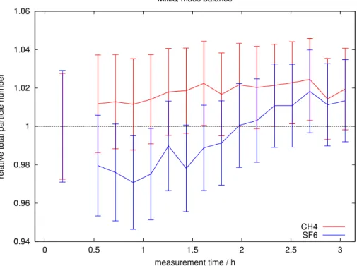
gas within the tank, for a typical exchange experiment. Deviations are within the error, proving that the setup is gas-tight, i.e. no gas is lost or acquired during the run.

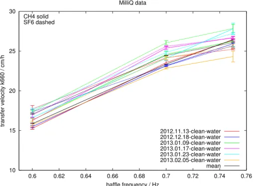
Estimated values ofk660 (kw scaled to a Schmidt number of 660) derived from CH4

and SF₆ for 6 diﬀerent MilliQ experiments are shown in Fig. 8. Weighted means and standard deviations of these data are summarised in Table 1. For individual

experi-5

ments the two independentk660estimates show very close agreement; any small

dis-crepancies most likely include uncertainties in the Schmidt number values and the solubility parameterisations. Thus, even in the worst case changes of 2 cm h−1are sig-nificant with 95 % probability; for the baﬄe speed of 0.6 Hz the significance level is 1.2 cm h−1 with 95 % probability. The weighted standard deviation is 4 % for all baﬄe

10

speeds and both gases.

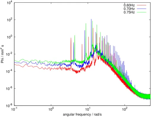
Wave spectra for a selected experiment are shown in Fig. 9. As expected, the wave energy is higher for higher baffle frequencies. The first peak for each boundary con-dition corresponds to the respective baffle speed, showing that the baffle has a repro-ducible and stable frequency. Further peaks at higher frequencies are the harmonics

15

caused by reflection and refraction inside the tank.

5.3 Seawater experiments

Estimated values of kw from the coastal North Sea transects, derived from CH4 at

a baﬄe speed of 0.6 Hz, are shown in Fig. 10 (top). For the winter transect (13 Febru-ary 2013) kw was between (12.4±0.3) cm h−

1

(near-shore) and (13.2±0.2) cm h−1

20

(off-shore), while corresponding autumn (4 October 2012) values were between (9.4±0.3) cm h−1 (near-shore) and (11.6±0.2) cm h−1 (off-shore). Comparison with Fig. 10 (bottom), which shows surfactant activity (SA) in the SML samples, clearly shows these spatial and temporal differences in kw to be a function of SA. The

spa-tial gradients inkw are consistent with a decreasing influence of terrestrially derived 25

surfactants in river outflow with distance oﬀshore. Higherkwsuppression by surfactant

(25)

OSD

11, 693–733, 2014

samples

Title Page

Tables Figures

◭ ◮

Back Close

Full Screen / Esc

Discussion

P

a

per

|

D

iscussion

P

a

per

|

Discussion

P

a

per

|

Discuss

ion

P

a

per

|

winter suppression presumably reflects lower SA arising from surfactant degradation processes.

For the most landwards station of the autumn transect (low kw) and the most oﬀ

-shore station from the winter transect (highkw), kw vs. baﬄe frequency is shown for

CH4 and SF6 in Fig. 11. The agreement between the two gases is acceptable, the 5

discrepancies being largely attributable to uncertainties in the Schmidt number param-eterisations, with additional small contributions arising from GC detector drift, which is somewhat larger for SF6 than for CH4. Nevertheless, the observed trends are clearly

significant within the analytical error. Our experimental procedures are evidently well suited to examine the relative natural variability ofk_wbetween seawater samples

con-10

taining varying levels of surfactant.

6 Conclusions

We have developed a laboratory gas exchange tank and associated analytical method-ology that enables fully automated, routine determination of the gas transfer velocities of SF6, CH4and N2O in natural seawaters under strictly controlled conditions of turbu-15

lence. Repeated experiments with MilliQ water demonstrated a typical measurement accuracy of 4 % fork_w. Experiments with natural seawater samples collected on two North Sea coastal transects showed a clear influence of surfactant activity on the strong spatial and temporal gradients inkw that we observed. During ongoing and planned

work, both in the coastal North Sea and in the open ocean, we aim to establish clear

20

relationships between kw, surfactant activity and biogeochemical indices of primary

productivity. In so doing we hope to better understand the spatio-temporal variabilty ofkw and thereby, to contribute valuable new insights into the air–sea gas exchange

process.

Acknowledgements. We wish to thank our colleagues in the workshop of the School of

Ma-25

(26)

Chem-OSD

11, 693–733, 2014

samples

Title Page

Tables Figures

◭ ◮

Back Close

Full Screen / Esc

Discussion

P

a

per

|

D

iscussion

P

a

per

|

Discussion

P

a

per

|

Discuss

ion

P

a

per

|

istry at Newcastle for manufacturing the equilibration vessel. We acknowledge and appreciate funding provided by the German Research Foundation in support of K Schneider-Zapp (DFG research fellowship) and we thank the UK Natural Environment Research Council (NERC) for awarding a NERC small grant NE/IO15299/1 to R Upstill-Goddard.

References 5

Asher, W. E.: The eﬀects of experimental uncertainty in parameterizing air-sea gas exchange using tracer experiment data, Atmos. Chem. Phys., 9, 131–139, doi:10.5194/acp-9-131-2009, 2009. 696

Bock, E. J., Hara, T., Frew, N. M., and McGillis, W. R.: Relationship between air–sea gas transfer and short wind waves, J. Geophys. Res., 104, 25821–25831, doi:10.1029/1999JC900200,

10

1999. 696

Bullister, J. L., Wisegarver, D. P., and Menzia, F. A.: The solubility of sulfur hexafluoride in water and seawater, Deep-Sea Res. Pt. I, 49, 175–187, doi:10.1016/S0967-0637(01)00051-6, 2002. 703, 705, 709

Ć_osović_{, B., and Vojvodi}ć_{, V.: The application of ac polarography to the determination of}

15

surface-active substances in seawater, Limnol. Oceanogr., 27, 361–369, 1982. 708

Crutzen, P. J. and Zimmermann, P. H.: The changing photochemistry of the troposphere, Tellus B, 43, 136–151, doi:10.1034/j.1600-0889.1991.t01-1-00012.x, 1991. 699

Dlugokencky, E. J., Masarie, K. A., Lang, P. M., and Tans, P. P.: Continuing decline in the growth rate of the atmospheric methane burden, Nature, 393, 447–450, 1998. 699

20

Dlugokencky, E. J., Walter, B. P., Masarie, K. A., Lang, P. M., and Kasischke, E. S.: Mea-surements of an anomalous global methane increase during 1998, Geophys. Res. Lett., 28, 499–502, doi:10.1029/2000GL012119, 2001. 699

Frew, N. M.: The role of organic films in air–sea exchange, in: The Sea Surface and Global Change, edited by: Liss, P. S. and Duce, R. A., Cambridge University Press, 121–172, 1997.

25

696

(27)

OSD

11, 693–733, 2014

samples

Title Page

Tables Figures

◭ ◮

Back Close

Full Screen / Esc

Discussion

P

a

per

|

D

iscussion

P

a

per

|

Discussion

P

a

per

|

Discuss

ion

P

a

per

|

Gašparović, B.: Decreased production of surface-active organic substances as a consequence of the oligotrophication in the northern Adriatic Sea, Estuar. Coast. Shelf Sc., 115, 33–39, doi:10.1016/j.ecss.2012.02.004, 2012. 696

Goldman, J. C., Dennett, M. R., and Frew, N. M.: Surfactant eﬀects on air–sea gas exchange un-der turbulent conditions, Deep-Sea Res., 35, 1953–1970,

doi:10.1016/0198-0149(88)90119-5

7, 1988. 696

Harnisch, J. and Eisenhauer, A.: Natural CF₄and SF₆on Earth, Geophys. Res. Lett., 25, 2401– 2404, doi:10.1029/98GL01779, 1998. 698

Harris, F. J.: On the use of windows for harmonic analysis with the discrete Fourier Transform, in: Proceedings of the IEEE, Vol. 66-1, 1978. 708

10

IPCC: Climate Change 2007 – The Physical Science Basis: Working Group I Contribution to the Fourth Assessment Report of the IPCC, Cambridge University Press, Cambridge, UK and New York, NY, USA, 2007. 695, 698

Jähne, B.: Air–sea gas exchange, in: Encyclopedia Ocean Sciences, edited by: Steele, J. H., Turekian, K. K., and Thorpe, S. A., 3434–3444, Elsevier,

doi:10.1016/B978-012374473-15

9.00642-1, 2009. 695

Khalil, M.: Atmospheric Methane: Sources, Sinks and Role in Global Change, Springer, New York, 1993. 699

Khatiwala, S., Primeau, F., and Hall, T.: Reconstruction of the history of anthropogenic CO₂ concentrations in the ocean, Nature, 462, 346–349, doi:10.1038/nature08526, 2009. 694

20

McKenna, S. P. and McGillis, W. R.: The role of free-surface turbulence and surfactants in air– water gas transfer, Int. J. Heat Mass Tran., 47, 539–553, 2004. 696

Nevison, C. D. and Holland, E.: A reexamination of the impact of anthropogenically fixed ni-trogen on Atmospheric N₂O and the stratospheric O₃layer, J. Geophys. Res., 102, 25519– 25536, doi:10.1029/97JD02391, 1997. 698

25

Nightingale, P., Malin, G., Law, C. S., Watson, A. J., Liss, P. S., Liddicoat, M. I., Boutin, J., and Upstill-Goddard, R. C.: In situ evaluation of air–sea gas exchange parameteriza-tions using novel conservative and volatile tracers, Glob. Biogeochem. Sci., 14, 373–387, doi:10.1029/1999GB900091, 2000. 695, 698

Phillips, O. M.: The Dynamics of the Upper Ocean, Cambridge University Press, New York,

30

1980. 714