Measuring air–sea gas-exchange velocities in a large-scale annular wind–wave tank

© Author(s) 2015. CC Attribution 3.0 License.

Measuring air–sea gas-exchange velocities in a large-scale annular

wind–wave tank

E. Mesarchaki1, C. Kräuter2, K. E. Krall2, M. Bopp2, F. Helleis1, J. Williams1, and B. Jähne2,3

1_{Max-Planck-Institut für Chemie (Otto-Hahn-Institut) Hahn-Meitner-Weg 1, 55128 Mainz, Germany} 2_{Institut für Umweltphysik Universität Heidelberg, Im Neuenheimer Feld 229, 69120 Heidelberg, Germany} 3_{Heidelberg Collaboratory for Image Processing (HCI), Universität Heidelberg, Speyerer Straße 6,}

69115 Heidelberg, Germany

Correspondence to:E. Mesarchaki (evridiki.mesarchaki@mpic.de) Received: 1 May 2014 – Published in Ocean Sci. Discuss.: 23 June 2014

Revised: 28 November 2014 – Accepted: 17 December 2014 – Published: 28 January 2015

Abstract. In this study we present gas-exchange measure-ments conducted in a large-scale wind–wave tank. Fourteen chemical species spanning a wide range of solubility (dimen-sionless solubility,α=0.4 to 5470) and diffusivity (Schmidt number in water, Scw=594 to 1194) were examined

un-der various turbulent (u10=0.73 to 13.2 m s−1) conditions.

Additional experiments were performed under different sur-factant modulated (two different concentration levels of Tri-ton X-100) surface states. This paper details the complete methodology, experimental procedure and instrumentation used to derive the total transfer velocity for all examined trac-ers. The results presented here demonstrate the efficacy of the proposed method, and the derived gas-exchange veloci-ties are shown to be comparable to previous investigations. The gas transfer behaviour is exemplified by contrasting two species at the two solubility extremes, namely nitrous oxide (N2O) and methanol (CH3OH). Interestingly, a strong

trans-fer velocity reduction (up to a factor of 3) was observed for the relatively insoluble N2O under a surfactant covered

wa-ter surface. In contrast, the surfactant effect for CH3OH, the

high solubility tracer, was significantly weaker.

1 Introduction

The world’s oceans are key sources and sinks in the global budgets of numerous atmospherically important trace gases, in particular CO2, N2O and volatile organic compounds

(VOCs) (Field et al., 1998; Williams et al., 2004; Millet et al., 2008, 2010; Carpenter et al., 2012). Gas exchange

be-tween the ocean and the atmosphere is therefore a signifi-cant conduit within global biogeochemical cycles. Air–sea gas fluxes, provided by either direct flux measurements or accurate gas transfer parameterisations, are a prerequisite for global climate models tasked to deliver accurate future pre-dictions (Pozzer et al., 2006; Saltzman, 2009).

The principles behind gas exchange at the air–sea interface have been reported in detail within previous reviews (Jähne and Haußecker, 1998; Donelan and Wanninkhof, 2002; Wan-ninkhof et al., 2009; Jähne, 2009; Nightingale, 2009). A sim-plified conceptual two layer model is generally accepted. The model assumes that close to the interface turbulent motion is suppressed and that the transfer of gases is controlled by molecular motion (expressed by the diffusion coefficientD). This leads to the formation of two mass boundary layers on both sides of the interface. In the upper part of the air-side mass boundary layer, turbulent transport becomes sig-nificant. Further away from the interface the significance of the air-side turbulent transport increases. In the water-side, due to lower diffusivities, molecular transport remains the controlling factor of the transfer. Depending on the solubil-ity of the gas in question, its transfer could be restricted by one or both sides of the interface (i.e air-side and water-side controlled).

The transfer velocity,k(in cm h−1), of a gas across the sur-face is defined as the gas flux density,F, divided by the con-centration difference,1c, between air and water (henceforth namedktexpressing the transfer through both boundary

lay-ers against the single air and water layer transfer,kaandkw,

as well as the resultant processes (surface stress and rough-ness, waves, breaking waves, bubbles, spray, etc.) influences the thickness of the mass boundary layers. Thus, the transfer velocity is related to the degree of turbulence on both sides close to the interface as well as the tracer characteristics, i.e. their solubility and diffusion coefficients (Danckwerts, 1951; Liss and Slater, 1974). Surface films are also known to have a strong influence on the transfer velocity by inhibiting waves and decreasing the near-surface turbulence (e.g Frew et al., 1990; Jähne and Haußecker, 1998; Zappa et al., 2004; Salter et al., 2011). To date, research on surface films (using dif-ferent film thicknesses and types) and their effect on trans-fer velocity is only in the very early stages. The impact of wind-driven mechanisms, surface films and diverse physio-chemical tracer characteristics on the gas-exchange rates can be studied in detail through transfer velocity measurements of individual species provided by the method proposed here. Such studies aim to improve our understanding of air–sea gas transfer and provide new insights into the theoretical back-ground.

Gas transfer velocities have been determined in both field studies (using mass balance, eddy correlation or controlled flux techniques) and laboratory experiments described in pre-vious gas-exchange reviews (Jähne and Haußecker, 1998; Donelan and Wanninkhof, 2002; Wanninkhof et al., 2009; Jähne, 2009; Nightingale, 2009) and references therein. Wind–wave tanks, in contrast to the open ocean, offer a unique environment for the investigation of individual mech-anisms related to the air–sea gas exchange under controlled conditions.

Mass balance methods have been applied in the field us-ing geochemical tracers (O2, 14C, Radon, for instance in

Broecker et al., 1985) and dual tracer (SF6,3He, for instance

in Watson et al., 1991; Wanninkhof et al., 1993) techniques. The main drawback of these approaches was the relatively low temporal resolution (Jähne and Haußecker, 1998). Fur-thermore, the transfer velocity measurements were based pri-marily on sparingly soluble tracers, and very few experimen-tal results of highly soluble trace gas transfer velocities are available.

In this study, gas-exchange experiments were performed in a state-of-the-art large-scale annular wind–wave tank. An ex-perimental approach based on mass balance has been devel-oped, whereby air- and water-side concentrations of various tracers are monitored using instrumentation capable of on-line measurement. For the first time, parallel measurements of total air and water-side transfer velocities for 14 individual gases within a wide range of solubility, have been achieved. Wind speed conditions (reported at 10 metres height, u10)

as low as 0.73 and reaching up to 13.2 m s−1 were inves-tigated. Supplementary parameters directly linked with the gas-exchange velocities, such as friction velocity and mean square slope of the water surface, were additionally mea-sured under the same conditions. This paper details the en-tire instrumental set-up and provides a validation of the

over-all operation and concept through transfer velocity measure-ments of nitrous oxide and methanol. These species are cho-sen as they bracket the wide range of solubilities among the investigated tracers and clearly show different gas-exchange behaviours. Transfer velocity measurements of the remain-ing examined tracers are goremain-ing to be presented in a follow-up publication.

2 Method

In this study, total transfer velocities for low as well as medium to highly soluble tracers were determined using a mass balance approach. The wind–wave tank is interpreted in terms of a box model.

2.1 The box model

The basic idea of the box model method is the development of a direct correlation between the air- and water-phase con-centrations,ca andcw, and the desired transfer rates,kt, of

various inert tracers.

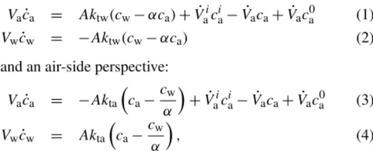
Figure 1 shows a schematic representation of the wind– wave tank in a box model (Kräuter, 2011; Krall, 2013). Wa-ter and air spaces are assumed to be two well-mixed separate boxes with volumes,VwandVa, between which tracers can

be exchanged only through the water surface,A. Further pos-sible pathways of tracers entering or leaving the box are also shown in Fig. 1. Assuming constant volumes, temperature and pressure conditions, the mass balance for the air and the water phases of the box yields for a water-side perspective:

Vac˙a = Aktw(cw−αca)+ ˙Vaicia− ˙Vaca+ ˙Vac0a (1)

Vwc˙w = −Aktw(cw−αca) (2)

and an air-side perspective:

Vac˙a = −Akta

ca− cw

α

+ ˙V_aici_a− ˙Vaca+ ˙Vaca0 (3) Vwc˙w = Akta

ca− cw

α

, (4)

whereα=cw/ca denotes the dimensionless solubility and ktw,kta the total transfer velocities for a water- and an

air-sided viewer, respectively. The two transfer velocities dif-fer by the solubility factor of the tracer (see Eq. A1 in Ap-pendix A). The dotting stands for the time derivative of the related symbol.

The first term on the right hand side of each equation rep-resents the exchange of a tracer from one phase to the other due to a concentration gradient. The second term stands for possible tracer input (V˙_aici_a), the third term for possible tracer output (flushing/leaking term:V˙aca) and the fourth term for a

possible tracer coming in through leaks from the surrounding room or through the flushing (V˙ac0a).

c_a

c_w

V ca

V

Va

V_w

k

V ca0

Figure 1.Mass balances for the air and water side. Naming con-vention is as follows: A: water surface area;Va: air volume;Vw: water volume; k: gas transfer velocity;ca: air-side concentration; cw: water-side concentration; cia: input tracer concentration; ca0: tracer concentration in the ambient air. The dotting denotes the time derivative of the related symbol.

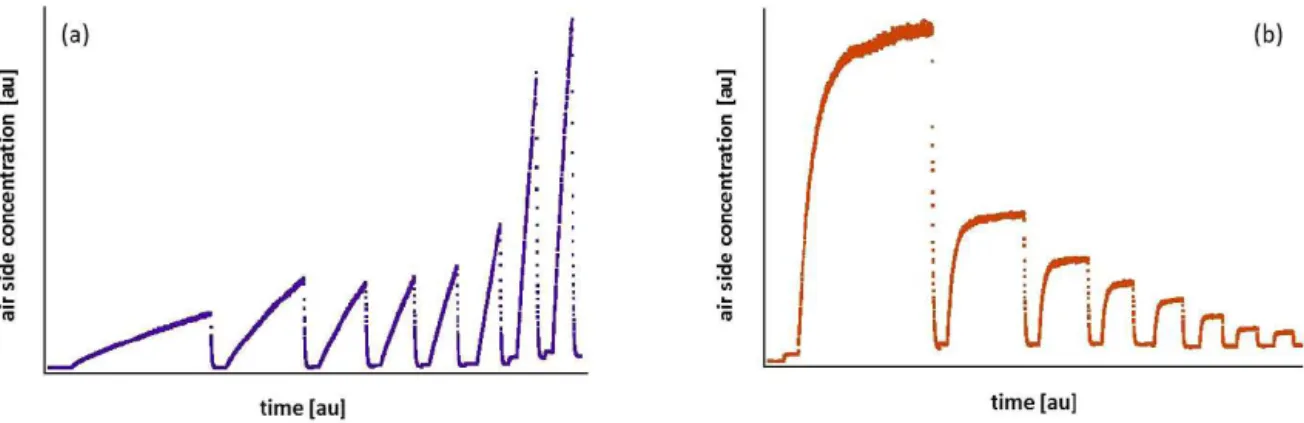
high solubility tracers (air-side controlled: Sect. 2.3), are pre-sented in detail. The simulated air/water concentration time series derived for a water-side (b and c in purple) and an air-side controlled (d and e in orange) tracer are presented in Fig. 2.

2.2 Water-side controlled tracers

The following approach was used for tracers with relatively low solubility (α <100) for which the transfer velocity,kt,

is mainly restricted due to the water-side resistance. Here, a low solubility tracer is dissolved in the water volume which is considered well mixed. High tracer concentration in the water and very low concentrations in the air (ca≃0) direct

the flux from the water to the air (evasion).

Figure 2b shows the simulated air-phase concentration time series of an example water-side controlled tracer at three example wind speed conditions (as seen in Fig. 2a, change of wind speed is denoted with grey dashed lines). Each condi-tion starts with a closed air-space tank configuracondi-tion (closed box – no flushing; see more details in Sect. 3.2.5), where the air-side concentration, starting from circa zero, increases lin-early with time, due to the water-to-air gas exchange. At time

t1, the air space is opened (open box – flushing on; flushing

time is denoted with grey background) and a drastic decrease is observed due to dilution of the air-space concentration with the relatively clean ambient air entering the facility. As indi-cated in the figure, the higher the wind speed the faster the concentration increase. Figure 2c presents the water-phase concentration of the same tracer which in parallel starts from the highest concentration point and gradually decreases dur-ing the course of the experiment as more and more molecules escape the water to enter the gas phase.

The ambient tracer concentration in the air entering the air space through leaks or during flushing can be safely assumed as negligible in comparison to the levels used for all exam-ined tracers. Omitting parameterc0_a, simplifies the box model Eq. (1), which can be subsequently solved forktwas follows: ktw=

Va A ·

˙

ca+λf,xca cw

· 1

1−αca/cw

, (5)

a)

wind spee

d

[au]

t₀ t1 t2

b)

a

ir

-side c

oncen

tr

a

tion

[au]

t0 t1 t2

c)

w

a

ter

-side

concen

tr

a

tion

[au]

t0 t1 t2

d)

a

ir

-side c

oncen

tr

a

tion

[au]

t0 t1 t2 SS1

SS 2

e)

w

a

ter

-side

concen

tr

a

tion

[au]

t0 t1 t2 time [au]

Figure 2.Simulated concentration time series for a water (b and

whereλf,x= ˙Va/Vais the leak or flush rate forxbeing 1 or

2, respectively.

Applying Eq. (5), the instantaneous total transfer veloc-ities (ktw) can be calculated from time-resolved

measure-ments of air- and water-side concentrations. 2.3 Air-side controlled tracers

In this approach, tracers with relatively high solubility (α >

100) for whichktis expected to be controlled mainly by

air-side processes, were used. Here, a relatively high solubility tracer is introduced with a constant flow to the air volume, continuously during the experiment. Due to low concentra-tions in the water volume, the net gas-exchange flux is di-rected from the air to the water (invasion).

In Fig. 2d the phase concentration of an example air-side controlled tracer is shown. During the closed air-space period (t0tot1), the concentration increases exponentially, as

a fraction of the air-space molecules transmit into the water due to the air–water gas exchange. At t1, the concentration

reaches a steady state, SS1, where the input rate of the tracer

is equal to the exchange rate between the two phases and the leak/flush rate.

At an equilibrium point, the concentration time derivative ˙

cais approximately zero so that Eq. (3) can be written as

ca=

λtac_αw+λicai λta+λf,x

, (6)

whereλta=_VA_aktais the exchange rate andλi= ˙ Vai

Va the input

rate.

After SS1, the facility is flushed with ambient air (open air

space) and the concentration decreases abruptly. Under these conditions (t2), a second steady state, SS2, is developed at a

lower concentration range. In SS1, a very small leak rate is

present (λf,1≈0, leak rate) while in SS2the leak rate is much

larger due to the open air space (λf,2, flush rate). Dividing the

air-side concentrations of the two steady states ca,1

ca,2 (as given

in Eq. 6) and solving it with respect to the exchange rate yields

λta=

λf,2ca,2−λf,1ca,1 (ca,1−ca,2)

. (7)

The total transfer velocities in the wind–wave tank box are calculated from

kta= λtaVa

A . (8)

2.3.1 Leak and flush rate

In most wind–wave facilities, small air leaks are inevitable. The amount of tracer escaping the air space of the facil-ity needs to be monitored and corrected for, as described in Sects. 2.2 and 2.3. To measure the leak/flush rate λf,x for

the open and closed configuration of the wind–wave tank, a

non-soluble tracer (here CF4), called a leak test gas, is used.

Directly after closing the wind–wave tank, a small amount of the leak test gas is injected rapidly into the air space. As the leak test gas is non-soluble, the water-side concentration,cw,

as well as the gas-exchange velocity,kta, in Eq. (3) are equal

to zero, reducing the air-side mass balance equation to

Vac˙a= ˙Vaic i

a− ˙Vaca. (9)

After the initial injection, the input termV˙_aic_ai in Eq. (9) van-ishes, yieldingVac˙a= − ˙Vaca. This simple differential

equa-tion can be solved easily with

ca(t )=ca(0)·exp(−λf,x·t ), (10)

whereca(0)is the concentration directly after the input of the

leak test gas. Monitoring the concentration of the leak test gas over time and fitting an exponentially decreasing curve to this concentration time series yields the leak/flush rateλf,x

of the system. In the Aeolotron facility, typical leak and flush rates were of the order of 0.05 to 0.4 h−1and 20 to 50 h−1, respectively.

3 Experiments

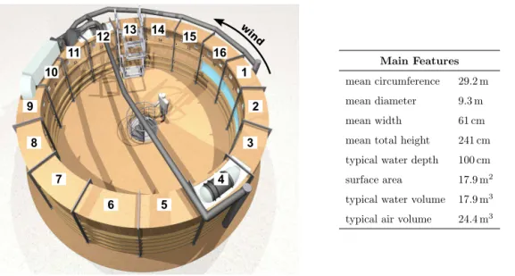
3.1 The Aeolotron wind–wave tank

The air–water gas-exchange experiments were conducted in the large-scale annular Aeolotron wind–wave tank at the Uni-versity of Heidelberg, Germany (Fig. 3). With an outer diam-eter of 10 m, a total height of 2.4 m and a typical water vol-ume of 18 000 L, the Aeolotron represents the world’s largest operational ring shaped facility (much larger than annular fa-cilities used in previous investigations, Jähne et al., 1979, 1987). The chamber is mostly gastight, thermally isolated, chemically clean and inert. In Fig. 3, a list of the main dimen-sions along with an aerial illustration of the facility are given. The tank is divided in 16 segments and an inner window ex-tending through segments 16 to 4 allows visual access to the wind formed waves. The facility ventilation system consists of two pipes through which the air space can be flushed with ambient air at a rate of up to 50 h−1. Two diametrically posi-tioned ceiling mounted axial ventilators (segment 4 and 12) are used to generate wind velocities of up touref=12 m s−1.

16 1

2

3

4 5

6 7

8 9

10

11 12 13 14 15

w in

d

Main Features

mean circumference 29.2 m

mean diameter 9.3 m

mean width 61 cm

mean total height 241 cm

typical water depth 100 cm

surface area 17.9 m2

typical water volume 17.9 m3

typical air volume 24.4 m3

Figure 3.An aerial illustration of the Aeolotron tank and its main features. The numbers denote the segments. The axial fans producing the wind can be seen in the roof of segments 4 and 12. The air pipes supplying fresh air and removing waste air are shown in grey; figure adapted from (Krall, 2013)).

The annular geometry of the wind–wave tank, contrary to a linear geometry, permits homogeneous wave fields and un-limited fetch. The well-mixed air space (at few centimetres height above the surface) ensures no concentration gradi-ents and therefore concentration measuremgradi-ents independent of the sampling height. On the other hand, the restricted size of the facility which leads to waves reflecting off the walls, results with a different wave field to that found in the open ocean.

3.2 Tracers and instrumentation

A series of 14 tracers covering a wide solubility (α=0.4 to 5470) and diffusivity (Scw=594 to 1194) range, were

se-lected for this study. Many of these tracers are very com-mon in the ocean environment, while the rest are used to extend the solubility and diffusivity ranges, a significant cri-terion for further physical investigations of the gas-exchange mechanisms. Table 1 gives an overview of the examined trac-ers, with their respective molecular masses, solubility and Schmidt numbers, Sc (the dimensionless ratio of the kine-matic viscosity of waterνand the diffusivity of the tracerD,

Sc=ν/D) at 20◦C.

All tracers were monitored on-line in both the air and the water phase. The VOC measurements were performed using proton reaction mass spectrometry (PTR-MS) from Ionicon Analytik GmbH (Innsbruck, Austria), while for the halocar-bons and N2O, two Fourier transform infrared (FT-IR)

Spec-trometers (Thermo Nicolet iS10) were used. As leak test gas, carbon tetrafluoride (CF4) was used; it was also measured by

FT-IR spectrometry.

For the surfactant experiments, the soluble substance Tri-ton X-100, C14H22O(C2H4O)9.5 (Dow Chemicals, listed

Mr= 647 g mol−1) was used to cover the water surface.

Tri-ton X-100 was chosen because of its common use as a refer-ence substance to quantify the surface activity of unknown surfactant mixtures found in the open ocean (Frew et al., 1995; Cosovic and Vojvodic, 1998; Wurl et al., 2011).

The operation and sampling conditions for both air and water phases are briefly described below. Additional instru-mentation for substantial supplementary measurements fol-lows.

3.2.1 Water-phase measurements

In the water phase a PTR-Quadrupole-MS (PTRQ-MS) (wa-ter inlet in segment 3) and a FT-IR spectrome(wa-ter (wa(wa-ter inlet in segment 6) were used to measure the concentration lev-els of the VOCs and the halocarbons and N2O, respectively.

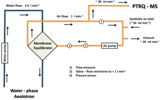
Our instrumentation, which is normally suited only for air sampling, was combined with an external membrane equi-librator (the oxygenator Quadrox manufactured by Maquet GmbH, Rastatt, Germany) to establish equilibrium between the water concentration and the gas stream to be measured. In this way, water-side concentrations could be obtained and used for the calculation of the transfer velocities for the low solubility tracers (see Sect. 2.2).

Membrane equilibrator configuration

Table 1.Molecular masses (Min g mol−1), dimensionless solubility (α) and Schmidt numbers in air (Sca) and water (Scw) for the investi-gated tracers at 20◦C.

Gas Formula M α Scl_a Scl_w

methanol CH₃OH 32.04 5293a 1.0268 671.04

1-butanol C4H9OH 74.12 4712b 1.8198 1141.7 acetonitrile CH3CN 41.05 1609c 1.2957 832.07 acetone (CH3)2CO 58.08 878.0c 1.4921 880.53 2-butanone C2H5COCH3 72.11 598.9b 1.7344 1159.8 acetaldehyde CH3CHO 44.05 378.7d 1.0786 824.90 ethyl acetate CH3C(O)OC2H5 88.10 156.4e 1.8183 997.46

dms CH3SCH3 62.13 16.62f 1.4484 979.40

benzene C6H6 78.11 5.672g 1.6785 980.46

toluene C6H5CH3 92.14 4.529g 1.8409 1176.3 trifluoromethane CHF3 70.01 0.760h 1.2132 747.50 nitrous oxide N2O 44.01 0.676i 1.0007 593.90 isoprene C5H8 68.12 0.31j–0.69k,∗ 1.6617 1193.9 pentafluoroethane CF3CHF2 120.0 0.415h 1.5106 1027.0

a_{Schaffer and Daubert (1969),}b_{Snider and Dawson (1985),}c_{Benkelberg et al. (1995),}d_{Betterton and}

Hoffmann (1988),e_{Janini and Quaddora (1986),}f_{Dacey et al. (1984),}g_{Robbins et al. (1993),}h_{Krall (2013),} i_{Weiss and Price (1980),}j_{Yaws and Pan (1992),}k_{Sander (1999),}l_{Yaws (1995),}∗_{only available values at 25}◦_C.

wind speed

flushing

water sided tracer input air sided tracer input

preparation phase measurement phase tt

t

t t

1 2 3 4 5 6 7 8

Figure 4.Schematic time series of the wind speed, flushing periods and air/water tracer inputs.

the partial pressure difference of the gases involved, until equilibrium between air and water is achieved (Henry’s law at constant temperature).

A detailed configuration of the membrane set-up in con-junction with the PTR-MS is shown in Fig. 6. The system consists of a water and an air loop, both constantly in con-tact with the membrane equilibrator. The dark blue lines

rep-resent the water loop where water was being pumped from the Aeolotron through the membrane and back into the fa-cility, with a constant flow of 3.4 L min−1. The light orange coloured lines represent the air loop which has a link to the PTRQ-MS instrument. A synthetic air inlet and an excess flow exhaust are used to regulate the flow inside the air loop constant at 1 L min−1_{and the systems pressure at 1013 hPa.}

Part of the air that comes out of the equilibrator is driven to the PTRQ-MS for analysis, while the rest remains in the loop. The relative humidity in the equilibrated air increases after passing through the equilibrator; therefore, the air tub-ing was heated to a few degrees above room temperature to avoid water condensation.

A similar set-up using a second membrane equilibrator was connected to the FT-IR instrument. The water flow was kept at a rate of about 3 L min−1. Here the instrument’s mea-suring cell was integrated into the air loop, removing the need for sample extraction, a synthetic air inlet and an ex-haust. The air was circulated in the closed loop at a rate of approximately 150 mL min−1. Between the equilibrator and the measuring cell, a dehumidifying unit containing phos-phorous pentoxide was used to remove water from the air stream and in this way protect the optical windows of the IR measuring cell.

The time constant of the membrane equilibrator was evalu-ated as described in Krall and Jähne (2014), providing a very fast response of≃1 min.

PTRQ-MS configuration

Figure 5.Air-side concentrations obtained for example water-side(a)and air-side(b)controlled tracers throughout the experimental proce-dure.

was operated under 30 mL min−1 sampling flow, 2.1 mbar drift pressure, and 600 V drift voltage (E / N=130 Td, Td=10−17cm2V molecule−1). A total of 30 masses were measured sequentially with a dwell time of 1 s (time reso-lution is 30 s). Possible mass overlapping was prevented by the careful reselection of the analysed compounds based on the initial mass scan.

Water-phase calibrations were performed in conjunction with the membrane equilibrator set-up (see Fig. 6). Known VOC concentrations were diluted in deionised water and then introduced into the water phase of the facility, in precise vol-ume quantities. To avoid losses of the investigated tracers into the air phase due to air–water gas exchange, the wa-ter surface was covered with a large amount of an organic surfactant (0.446 mg L−1, Triton X-100) and calm wind con-ditions were used to gently mix the air space. Under such conditions gas-exchange velocities were estimated to be neg-ligible. Linear behaviour was established for all examined tracers at concentration levels embracing the characteristic water-phase concentration ranges detected during the exper-iments.

FT-IR configuration

The key aspects of FT-IR spectroscopy are described in de-tail in Griffiths (2007). In this study, a Nicolet iS10 (manu-factured by Thermo Fischer Scientific Inc., Waltham, MA., USA) FT-IR spectrometer with a custom made measuring cell of approximately 5 cm length was used. About every 5 s, one infrared absorbance spectrum with wave numbers be-tween 4000 and 650 cm−1with a resolution of 0.214 cm−1 was acquired. Six of these single spectra were averaged to minimise noise and stored for further evaluation, leading to a time resolution of about 1 spectrum every 30 s. Signal con-version to water-phase concentration, calibration and uncer-tainty estimation are described in detail in Krall (2013).

3.2.2 Air-phase measurements

In the air phase, a PTR-time of flight (ToF)-MS (inlet in seg-ment 3) with a time resolution of 10 s provided very fast on-line measurements for the VOCs while a FT-IR (inlet in seg-ment 2) with a time resolution of 30 s was in parallel monitor-ing the halocarbons and N2O. High time resolution

measure-ments enabled a fast experimental procedure and at the same time high accuracy data analysis. Additionally, due to the fast on-line measurements, the transient response of the system could be followed very efficiently throughout the experimen-tal procedure. Example air-side measurements are shown in Fig. 5 for a water and an air-side controlled tracer.

PTR-ToF-MS configuration

The ionisation principle of the PTR-ToF-MS is the same as the PTRQ-MS; however, here a time-of-flight mass spec-trometer is used. Throughout the measurements, the PTR-ToF-MS was configured in the standard V mode with a mass resolution of approximately 3700 m1m−1. The drift voltage was maintained at 600 V and the drift pressure at 2.20 mbar (E / N140 Td). Mass spectra were collected over the range 10–200m/z(mass-to-charge ratio) and averaged every 10 s, providing a mean internal signal for each compound. Af-ter acquisition all spectrum files were mass calibrated using (H2O)H+, NO+ and (C3H6O)H+ ions to correct for mass

peak shifting.

Calibrations in the air phase were conducted under high humidity conditions equivalent to the sampling conditions during the experiments (85–90 % RH). The desired mixing ratios (1–600 ppbv) were obtained by appropriate dilution of the multi-component VOC gas standard with synthetic air. Linear response was established for all examined tracers. FT-IR configuration

was kept at a constant temperature of 35◦C using a Thermo Nicolet cell cover. Air from the Aeolotron was sampled at a rate of 150 min−1at segment 13. As with the water-side in-strumentation, water vapour was removed before entering the measuring cell using phosphorous pentoxide. The spectrom-eter settings, data acquisition as well as data processing, were identical to the water-side instrumentation, see Sect. 3.2.1. 3.2.3 Error analysis ofkt

The individual total transfer velocity uncertainties were cal-culated applying the propagation of error for uncertainties in-dependent from each other to Eq. (5) for thektw, and Eqs. (7)

and (8) for thekta.

The concentration uncertainties for the PTR-MS measure-ments were calculated using the background noise and the calibration uncertainty of each examined tracer. Relatively low uncertainties were obtained for the air-phase concentra-tion levels SS1and SS2ranging between 1–1.5 % and 1.5–

2.5 %, respectively. The water-phase concentration uncer-tainty,1cw, was estimated the same way and the

uncertain-ties were between 6.5 and 8 % for the concentration ranges used.

The uncertainty of the concentration measurement with the FT-IR spectrometers was found to be concentration de-pendent. All concentration uncertainties lie below 4 % for the typical concentrations measured in the described experi-ments.

The individual uncertainties for the leak and flush rates of all conditions were of the order of 0.5 and 1 %, respec-tively. Based on the geometrical parameters of the facility the surface area uncertainty was calculated to be approximately 2 %, while a maximum of 3 % is estimated for the volume un-certainty. For the solubility values provided by literature, ac-curate uncertainty estimations are difficult. Here we assume a maximum uncertainty of 10 % for all literature sources.

The overall estimated total transfer velocity uncertainties therefore ranged between 6–12 and 6–20 %, respectively, for thektaandktwvalues of all examined tracers.

3.2.4 Additional instrumentation

Supplementary measurements of wind driven, surface asso-ciated, physical parameters, such as the mean square slope and the water-sided friction velocity, were additionally made in the Aeolotron wind–wave tank to enable further investiga-tions of the physical mechanisms of air–water gas exchange. The mean square slope measurements, reflecting the sur-face roughness conditions, were performed in parallel with the gas-exchange measurements using a colour imaging slope gauge (CISG) installed in segment 13. The CISG de-vice uses the refraction properties of light at the air–water boundary. A colour coded light source was placed below the water while a camera observed the water surface from above. Using lenses to achieve a telecentric set-up, a relationship

between surface slope and the registered colour can be deter-mined. Errors are calculated from the statistical fluctuations of the individually measured mean square slope values. A more detailed description can be found in Rocholz (2008).

The water-sided friction velocity,u∗,w, measurements,

ex-pressing the shear stress created on the water interface, were accomplished at a later stage using the same setting of the wind generator and the same surfactant coverage of the wa-ter surface. The momentum balance method was used as de-scribed in Bopp (2014) and Nielsen (2004). To apply this method, the friction between the water and the walls needs to be measured first. This is done by monitoring the decrease of the velocity of the bulk water after switching off the wind. In a stationary equilibrium, that is characterised by an equal-ity of the momentum input into the water by the wind and the momentum loss due to friction at the walls, the friction velocity,u∗,w, can be calculated from the mean water

ve-locity. The water velocity was measured using a three-axis Modular Acoustic Velocity Sensor (MAVS-3 manufactured by NOBSKA, Falmouth, MA, USA) installed in the centre of the water channel in segment 4 of the Aeolotron at a water depth of around 50 cm. The uncertainty of the friction ve-locity measurements is calculated from the statistical fluctu-ations of the bulk water velocity measurement as well as the uncertainty in the friction parameter used in the momentum balance method. Both sources of error are described in de-tail in Bopp (2014). Subsequently, simple error propagation was used to derive the wind speed (u10) uncertainty from

the Smith and Banke (1975) empirical relationship (see Ap-pendix B), the error of which is assumed to be negligible. 3.2.5 Experimental arrangement

The Aeolotron facility was filled to 1 m height (∼18 m3 wa-ter volume) with clean deionised wawa-ter. Diluted aqueous mix-tures of low solubility tracers were introduced into the water phase of the facility a day prior to an experiment and homo-geneity was achieved using two circulating pumps. Before the beginning of each experiment (for the clean water surface cases), the water surface was skimmed to clean off any pos-sible surface contamination. To do this, a small barrier with a channel is mounted between the walls of the tank, perpen-dicular to the wind direction while the wind is turned on at a low wind speed (uref≈3 m s−1). The wind pushes the water

surface over the barrier into the channel removing any sur-factant. A pump continuously empties the channel and drains the water contaminated with surface active materials.

Individual gas-washing bottles containing highly solubil-ity tracers in liquid form were purged with a controlled flow of clean air that swept the air-tracer gas mixture into the air phase of the facility. The bottles were kept in a thermostatic bath at 20◦C throughout the experimental procedure.

W

a

ter

pump

Water flow: 3.4 l min-1

PTRQ - MS

Synthetic air inlet (~ 50 ml min-1₎

Air pump

1

2 3

1) Flow measure

2) Valve – flow restriction to ≈ 1 l min-1

3) Presure sensor Air flow: 1 l min-1

Membrane Equilibrator

Exhaust ~ 20 ml min-1

Water - phase Aeolotron

Figure 6.Membrane equilibrator – PTRQ-MS set-up schematic. The dark blue and orange lines represent the water and air loops of the system, accordingly.

point for all tracers. Thereafter, the flushing was turned off (closed air space) and the tracer concentration (air and water-side controlled) started to increase (see more in Sect. 2.3). Immediately after turning off the flushing, the leak test gas was introduced into the air space. After the steady-state point (SS1) for the air-side controlled tracers was approached, the

air space was flushed once more with ambient air and an abrupt concentration decrease was observed. The same pro-cess was repeated for eight different wind speed conditions, progressing from lower to higher values. In Fig. 4 a time se-ries of the experimental conditions (wind speed, flushing pe-riods and air and water tracer inputs) are schematically repre-sented. The obtained air-sided concentration time series over the eight wind speed conditions for a water- and an air-sided example tracer are given in Fig. 5.

The wind speed varied from very low values (uref=0.74 m s−1, equivalent to u10=0.73 m s−1) up

to higher ones (uref=8.26 m s−1, equiv.u10=13.2 m s−1).

At the very beginning of the experiment, hardly any surface movement was seen. As the experiment progressed, the first capillary waves became apparent and started breaking above uref=4.8 m s−1, equiv. u10=6.6 m s−1. Reaching

larger wavelengths, wave braking and bubble formation was observable only at the highest wind speed condition.

The experimental procedure described above was repeated four times at clean surface conditions for all tracers listed in Table 1. Three further repetitions were accomplished with a surfactant (Triton X-100) covered water surface. The surfac-tant concentration in the fifth repetition was 0.033 mg L−1 while in the last two a larger amount of 0.167 mg L−1 was used.

Despite the well-reproduced experimental conditions, small variations between the repetitions were observed. Ta-ble 2 displays a mean value of the main measured parameters along with the standard deviation, expressing the extent of variability between the repetitions, of each case. For the high-est wind speed condition of the clean case, only three repe-titions were performed. Also in repetition two, theσ_s2values observed in conditions 4, 5 and 6 were significantly lower and therefore omitted from the averaging. Here we assume that the water surface was probably insufficiently skimmed before the experiment or that surfactant material might have entered the facility during the flushing phases. In the higher surfactant case (case 3), the first condition was omitted for reasons of experimental simplicity while σ_s2 are available only for one repetition.

4 Results

In this work, total transfer velocities of two contrasting trac-ers at opposite ends of the solubility spectrum, N2O (α=

0.67) anticipated as only water-side controlled (i.ektw∼kw)

and CH3OH (α=5293) similarly anticipated as only air-side

controlled (i.e.kta∼ka), are presented. In this way, we intend

Table 2.Reference velocities,uref(m s−1), friction velocities,u∗,w(cm s−1), mean square slope,σs2, air temperature,ta(◦C), water tem-perature,tw(◦C) mean values and % standard deviations as quantified in the Aeolotron facility for case 1: clean surface experiments; case 2: surface covered with 0.033 mg L−1Triton X-100; and case 3: surface covered with 0.167 mg L−1Triton X-100, at eight different wind speed conditions. The number of replicates used for each case is given in brackets.

Case Parameter Cond.1 Cond.2 Cond.3 Cond.4 Cond.5 Cond.6 Cond.7 Cond.8

uref(±%) 0.744 (1.3) 1.421 (0.5) 2.052 (0.3) 2.674 (0.5) 3.621 (0.1) 4.805 (0.3) 6.465 (0.2) 8.256 (0.1) u∗,w(±%) 0.063 (1.4) 0.135 (0.6) 0.216 (0.4) 0.309 (0.6) 0.473 (0.2) 0.720 (0.5) 1.141 (0.3) 1.967 (0.1) 1 σ_s2(±%) 0.002 (1.7) 0.007 (1.4) 0.013 (1.2) 0.016 (0.5) 0.024 (2.2) 0.046 (2.0) 0.078 (3.0) 0.118 (6.3) (×4) ta(±%) 21.29 (1.5) 21.18 (1.5) 21.09 (1.6) 20.99 (1.6) 20.88 (1.6) 20.75 (1.6) 20.59 (1.7) 20.50 (1.8) tw(±%) 19.30 (1.7) 19.37 (1.8) 19.41 (1.8) 19.41 (1.8) 19.39 (1.8) 19.34 (1.9) 19.29 (2.0) 19.26 (2.1)

uref(±%) 0.800 ( – ) 1.460 ( – ) 2.091 ( – ) 2.717 ( – ) 3.650 ( – ) 4.851 ( – ) 6.502 ( – ) 8.288 ( – ) u∗,w(±%) – 0.163 ( – ) 0.246 ( – ) 0.336 ( – ) 0.484 ( – ) 0.698 ( – ) 1.038 ( – ) 1.464 ( – ) 2 σ_s2(±%) 0.002 ( – ) 0.002 ( – ) 0.002 ( – ) 0.008 ( – ) 0.010 ( – ) 0.020 ( – ) 0.071 ( – ) 0.111 ( – ) (×1) ta(±%) 22.11 ( – ) 22.04 ( – ) 21.94 ( – ) 21.77 ( – ) 21.64 ( – ) 21.44 ( – ) 21.19 ( – ) 21.11 ( – ) tw(±%) 19.80 ( – ) 19.88 ( – ) 19.93 ( – ) 19.93 ( – ) 19.93 ( – ) 19.90 ( – ) 19.88 ( – ) 19.85 ( – )

uref(±%) – 1.451 (1.2) 2.075 (0.0) 2.707 (0.6) 3.667 (0.3) 4.913 (0.4) 6.615 (0.2) 8.371 (0.0) u∗,w(±%) – 0.18 (1.0) 0.239 (0.0) 0.295 (0.5) 0.381 (0.3) 0.524 (0.7) 0.84 (0.4) 1.407 (0.1) 3 σ_s2(±%) – 0.002 ( – ) 0.002 ( – ) 0.002 ( – ) 0.005 ( – ) 0.007 ( – ) 0.040 ( – ) 0.096 ( – ) (×2) ta(±%) – 21.51 (1.4) 21.59 (1.3) 21.60 (1.0) 21.53 (0.9) 21.51 (0.6) 21.34 (0.7) 21.22 (0.9) tw(±%) – 19.83 (0.5) 19.86 (0.6) 19.90 (0.7) 19.94 (0.6) 19.95 (0.7) 19.95 (0.7) 19.95 (0.7)

4.1 Gas-exchange transfer velocities

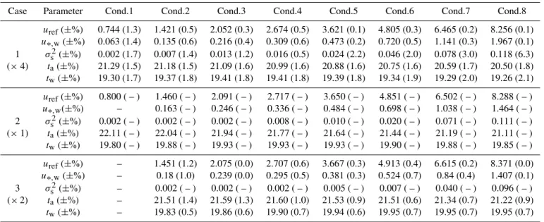
In Figs. 7 and 8, we present the experimentally obtainedktw

for N2O and kta for CH3OH as a function of u∗,w for the

clean water surface experiments. In both figures, the exper-imental results of all repetitions are nicely reproduced. Oc-casionally, the variation between the transfer velocity values exceeded the given uncertainty bars. A more apparent exam-ple is provided by the lower transfer velocity points (circles) at conditions 4, 5 and 6 which arise as a result of the lowerσ_s2

values observed in repetition 2 (as described in Sect. 3.2.5). This effect could be taken as an indication that only one phys-ical parameter is not enough to effectively describe the com-plicated process of the air–sea gas exchange. As the exper-imental conditions used in the four repetitions were similar but not identical (see Table 2), a four replicate mean value calculation was avoided and instead a fit through all points is chosen (black dashed line).

As indicated in Fig. 7, thektwincreases non-linearly with u∗,w. The correlation could be described as linear up to u∗,w=0.72 cm s−1(equiv.u10=6.6 m s−1) while above this

point, a faster increase is observed. This sudden increase in the so far linear tendency can be attributed to various wa-ter surface effects (e.g. initiation of capillary wave braking), which are not going to be discussed here.

The air-sided transfer velocities kta (Fig. 8) in

con-trast, increase linearly (R2=0.99) with u∗,w throughout

the examined velocity range (u∗,w=0.063–1.7 cm s−1equiv. u10=0.73–13.2 m s−1). As it appears from Fig. 8, the first

transfer velocity values of CH3OH (i.e. those at the lowest

turbulent condition) are slightly underestimated relative to

the linear trend (≃10 %). This could be explained as being due to the inefficiently mixed air space caused by the lower turbulence conditions applied.

Overall, the observed trends and transfer velocity magni-tudes of bothktwandktaare in good agreement with

observa-tions made by previous studies. A more detailed comparison with literature follows in Sect. 4.3.

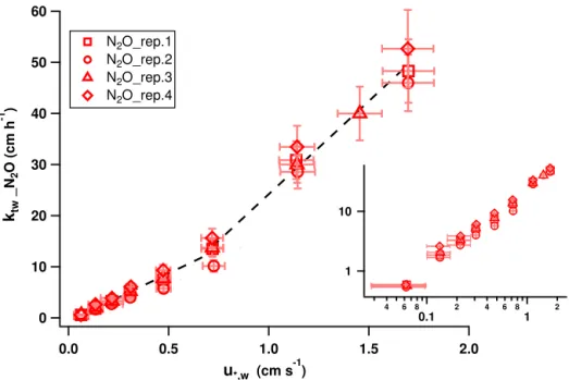
4.2 Effect of surfactants

After obtaining clear, reproducible transfer velocity trends for a clean water surface, the effect of a surfactant was evalu-ated using two different surfactant (Triton X-100) concentra-tions. As expected, the surfactant suppressed the transfer ve-locity as well as the friction veve-locity,u∗,w, and mean square

slope,σ_s2(see Table 2). In Fig. 9, the transfer velocities of all seven experiments for N2O and CH3OH are presented

against the reference wind speed,uref; a parameter which is

not affect by the surfactant layers.

As indicated in Fig. 9, the surfactant effect shows signifi-cant differences between the two contrasting tracers. A gen-erally stronger suppression is observed for N2O and a

sig-nificantly weaker for CH3OH where the transfer is mainly

controlled by the air-side boundary layer. Under low turbu-lence conditions, the surfactant diminished the transfer ve-locity of N2O by a factor of 3 for both examined

concen-trations (0.033 and 0.167 mg L−1Triton X-100) (Fig. 9a). In the case of CH3OH, the effect was weaker demonstrated by

a factor of 1.5 (Fig. 9b). At slightly higher wind speeds (i.e ≥uref3 m s−1; see Table 2 for the equivalentu∗,w of each

60

50

40

30

20

10

0 ktw

_

N2

O (cm h

-1 )

2.0 1.5

1.0 0.5

0.0

u_*,w (cm s-1)

N2O_rep.1 N2O_rep.2 N2O_rep.3 N2O_rep.4

1 10

4 6 8

0.1 2 4 6 81 2

Figure 7.Total transfer velocity of N₂O of four clean case repetitions plotted againstu∗,w. Squares correspond to repetition 1, circles to repetition 2, triangles to repetition 3 and diamonds to repetition 4. Vertical bars in light red give the individual transfer velocity uncertainty (see Sect. 3.2.3) and the horizontal bars the uncertainty of theu∗,wmeasurements.

14x103

12

10

8

6

4

2

0 kta

_

CH

3

OH (cm h

-1 )

2.0 1.5

1.0 0.5

0.0

u_*,w (cm s-1)

CH3OH_rep.1 CH₃OH_rep.2 CH₃OH_rep.3 CH₃OH_rep.4

4 6

103

2 4 6

104

4 6 8

0.1

2 4 6 8

1

2

Figure 8.Total transfer velocity of CH₃OH of four clean case repetitions plotted againstu∗,w. Symbols and bars are the same as in Fig. 7.

surfactant concentrations with the higher concentration caus-ing a more prominent suppression. Reachcaus-ing the highest ex-amined wind speed where waves, wave breaking and bub-bles are present, the surfactant effect is significantly weaker. In the case of CH3OH, no further impact is observed (values

within the error bars), while a still significant suppression (around a factor of 1.5) is apparent for thektwof N2O under

a 0.167 mg L−1Triton X-100 surfactant film.

Reduced surface stress and roughness change the hydrody-namic properties of the water surface and consequently affect the gas transfer. As given in Table 2, the suppression caused by a surfactant seems to be relatively strong forσ_s2(like in the case of N2O) and rather weak foru∗,w(here, note the higher

uncertainties at the low wind speed regime). The trend of the reduction for bothu∗,w andσs2was similar to the one ofkt,

4 6 103 2 4 6 104

4 6 8

0.1 2 4 6 81 2

1 2 3 4 5 6 10 2 3 4 5 6 100 ktw _N 2

O (cm h

-1 )

2 3 4 5 6 7 8 9

10 uref (m s

-1

)

clean surface 0.033 mg L-1 Triton-X100 0.167 mg L-1 Triton-X100

50 40 30 20 10 10 8 6 4 2 0 4 6 103 2 4 6 104

4 6 8

0.1 2 4 6 81 2

1 2 3 4 5 6 10 2 3 4 5 6 100 ktw _N 2

O (cm h

-1 )

2 3 4 5 6 7 8 9

10 u_ref (m s-1)

clean surface 0.033 mg L-1 Triton-X100 0.167 mg L-1 Triton-X100

50 40 30 20 10 10 8 6 4 2 0 7 8 9 103 2 3 4 5 6 7 8 9 104 kta _ CH 3

OH (cm h

-1 )

2 3 4 5 6 7 8 9

10 uref (m s

-1

)

clean surface

0.033 mg L-1 Triton-X100 0.167 mg L-1 Triton-X100

14 12 10 8 6 4 2 x10 3 10 8 6 4 2 0 (a) (b)

Figure 9.Effect of the two different surfactant concentrations on the total transfer velocities of(a)N2O and(b)CH3OH. The clean water surface results are given in red, the results obtained using 0.033 mg L−1Triton X-100 in green and the ones using 0.167 mg L−1Triton X-100 in blue.

turbulence. The way in which each of these parameters affect the gas transfer needs further investigation and is going to be presented in a following publication.

4.3 Comparison with previous studies

The gas transfer velocities of weakly soluble tracers has been extensively studied over the previous years. Numerous kw

parameterisations are available, derived from experimental (laboratory and field) measurements as well as physical mod-els. In Fig. 10, a selection of some representative, experi-mentally derived parameterisations (coloured lines), are used for comparison with thektw(herektw∼kw) measurements of

N2O (red points). The transfer velocities are plotted against

the wind speed at 10 m height,u10.

Looking at the lower wind speed range (0.7 to 4 m s−1) an obvious spread between the variouskwpredictions can be

convec-0.1 1 10 100

k

_N

2

O (cm h

-1 )

14 12

10 8

6 4

2 0

u

LM_86 M_01 C_94 M_04 WM_99 Ho_06 N_00 W_09 this study

80

60

40

20

0

14 12 10 8 6 4 2 0

Figure 10.Comparison between the N2O measurements of this study (red circles) and previouskwparameterisations. The coloured lines correspond to LM_86: Liss and Merlivat (1986); C_94: Clark et al. (1994); WM_99: Wanninkhof and McGillis (1999); N_00: Nightingale et al. (2000); M_01: McGillis et al. (2001); M_04: McGillis et al. (2004); Ho_06: Ho et al. (2006); and W_09: Wanninkhof et al. (2009).

tion can provoke an increase in the gas exchange which at very low wind speeds is considered significant. Such envi-ronmental differences could provide an additional explana-tion for the huge disagreement observed. The projected ab-solute quantity differences to the atmospheric budgets, how-ever, are estimated to be small since the fluxes themselves are small. The middle wind speed range seems to be well represented in all studies. At the higher wind speed range, a smaller spread was observed especially above 10 m s−1. This spread, a little more than an order of 2, can lead to great dis-crepancies in the atmospheric budgets of the related tracers as the corresponding transfer velocities are much larger there. The transfer velocities obtained in this study, show a closer agreement with the Clark et al. (1994) parameterisation apart from the lowest wind speed. There, our results agree better with Nightingale et al. (2000).

In contrast to the weakly soluble gases, high solubility tracers have received much less attention. In Fig. 11, the total transfer velocity measurements of CH3OH (herekta∼ka) are

compared with some available tunnel (Liss, 1973; Mackay and Yeun, 1983, coloured lines) and model (Duce et al., 1991; Jeffery et al., 2010, from COARE Algorithm; Fairall et al., 2003, grey lines)kaparameterisations as well as a recent

CH3OH field study (Yang, 2013, black line with triangles).

As indicated in Fig. 11, our results agree very well with the previous laboratory parameterisations lying nearer to Mackay and Yeun (1983). Here again the first transfer

veloc-ity point deviates, though an increase by the estimated 10 % would still not change this trend. We note that also in the case ofka, the lower wind speed range of the other

experi-mental studies is covered by a fit extension based on transfer velocities obtained at higher wind speeds.

The transfer velocity values provided by model and field studies are about 1.5 to 2 times lower than the ones derived from the laboratory measurements. This is to be expected as model and field studies include an extra turbulent resistance in the air space at 10 m height.

5 Conclusions

0.1 1 10 100

k

_N

2

O (cm h

-1 )

14 12

10 8

6 4

2 0

u

LM_86 M_01 C_94 M_04 WM_99 Ho_06 N_00 W_09 this study

80

60

40

20

0

14 12 10 8 6 4 2 0

102 2 3 4 5 6 103

2 3 4 5 6 104

ka

_CH

3

OH (cm h

-1 )

14 12

10 8

6 4

2 0

u₁₀ (m s-1)

L_73 D_91 MY_83 D_91* Y_13 J_10 this study

14

12 10

8

6 4

2 0

x10

3

14 12 10 8 6 4 2 0

Figure 11.Comparison between the CH3OH measurements of this study (red circles) and previouskaparameterisations. Experimental studies are presented with coloured lines: L_73: Liss (1973); MY_83: Mackay and Yeun (1983); and Y_13: Yang (2013), while model studies are given with grey lines: D_91 using theM; D_91∗using theSca: Duce et al. (1991); and J_10: Jeffery et al. (2010) using a Smith and Banke (1975) derived drag coefficient term.

complete data set for all species (including the intermediate cases of both layer control) along with the available micro-scale surface property parameters, extending over a low to medium wind speed regime, can be used to generate a gen-eralised parameterisation for the total transfer velocity. The derivation of this expression, which will be invaluable to fu-ture modelling efforts, will be presented in a separate publi-cation.

Particularly interesting are the effects on the gas transfer velocity induced by the addition of a surfactant. Despite the surface micro-layer being commonly present on the ocean, its effect on air–sea gas transfer is poorly understood and there is a paucity of data both from the laboratory and the field. The impact of the surfactant is markedly different on the two tracers shown here. A strong reducing effect (up to a factor of 3) was observed for the water-side controlled tracer, N2O while in the case of CH3OH, the surfactant showed a

quite weaker impact.

We maintain that it is important to monitor the transfer process in both the water-phase (using water-side controlled tracers) and the air-phase layer (using air-side controlled tracers) in order to develop a true enduring and generally ap-plicable model for air–sea gas transfer. The results produced here correspond reasonably well with previous expressions for ka andkw. In case ofkw, at low wind speeds there is a

wide spread in the literature values, with this study

corre-sponding most closely with those of Clark et al. (1994) and Nightingale et al. (2000). At high wind speeds the previous parameterisations are divided into three groups and this study lies in the central group. Despite the relatively small number of investigations, in case ofka, the literature spread is much

smaller with our results nicely corresponding to the previous laboratory parameterisations (i.e. Liss, 1973; Mackay and Yeun, 1983).

Appendix A: Relationship between air-sided and water-sided variables

The experimentally calculated water-sided total transfer ve-locities,ktw, were converted to the equivalent air-sided total

transfer velocities,kta, using

kta=αktw. (A1)

Air-sided friction velocities can be converted to water-sided friction velocities by

u∗,w= r_ρ

a ρw

u∗,a. (A2)

Appendix B: u10derivation usingu∗,a

The wind speed at a height of 10 m,u10, is calculated from its

relationship with the air-sided friction velocity and the drag coefficient,Cd, using

Cd= u∗,a2

u₁₀2

. (B1)

Here, the Smith and Banke (1975) empirical relationship be-tween the drag coefficient and the wind speed was used 103Cd=0.63+0.066u10. (B2)

Appendix C: Naming conventions

kw transfer velocity in water for a water-sided viewer ka transfer velocity in air for an air-sided viewer ktw total transfer velocity for a water-sided viewer kta total transfer velocity for an air-sided viewer cw water-side concentration

ca air-side concentration Vw water volume Va air volume A water surface λf,1 leak rate λf,2 flush rate α=cw

ca dimensionless solubility Scw Schmidt number in water Sca Schmidt number in air M molecular mass

Acknowledgements. We own a special thank to J. Auld and T. Klüpfel for their valuable assistance and support during the gas exchage experiments. The mean square slope values were kindly provided by R. Rocholz. R. Sander is thanked for the helpful and insightful discussions on solubility matters considering this manuscript. Furthermore, we thank all members of B. Jähne’s group for their understanding and support during the measurements. We acknowledge the financial support of the BMBF Verbundprojekt SOPRAN (www.sopran.pangaea.de; SOPRAN grant 03F0611A, 03F0611K, 03F0611F and 03F0662F)

The service charges for this open access publication have been covered by the Max Planck Society.

Edited by: J. Shutler

References

Benkelberg, H. J., Hamm, S., and Warneck, P.: Henry’s law coef-ficients for aqueous solutions of acetone, acetaldehyde and ace-tonitrile, and equilibrium constants for the addition compounds of acetone and acetaldehyde with bisulfite, J. Atmos. Chem., 20, 17–34, doi:10.1007/Bf01099916, 1995.

Betterton, E. A. and Hoffmann, R. M.: Henry’s law constants of some environmentally important aldehydes., Environ. Sci. Tech-nol., 22, 1415–1418, doi:10.1021/Es00177a004, 1988.

Bopp, M.: Luft und wasserseitige Strömungsverhältnisse im ringförmigen Heidelberger Wind-Wellen-Kanal (Aeolotron), Master Thesis, University of Heidelberg, available at: http://www.ub.uni-heidelberg.de/archiv/16962 (last access: 18 June 2014), 2014.

Broecker, W. S., Peng, T. H., Ostlund, G., and Stuiver, M.: The Dis-tribution of Bomb Radiocarbon in the Ocean, J. Geophys. Res.-Oceans, 90, 6953–6970, doi:10.1029/Jc090ic04p06953, 1985. Carpenter, L. J., Archer, S. D., and Beale, R.: Ocean-atmosphere

trace gas exchange, Chem. Soc. Rev., 41, 6473–6506, 2012. Clark, J. F., Wanninkhof, R., Schlosser, P., and Simpson, H. J.:

Gas-Exchange Rates in the Tidal Hudson River Using a Dual Tracer Technique, Tellus B, 46, 274–285, 1994.

Cosovic, B. and Vojvodic, V.: Voltammetric analysis of surface active substances in natural seawater, Electroanalysis, 10, 429– 434, doi:10.1002/(SICI)1521-4109(199805)10:6<429::AID-ELAN429>3.0.CO;2-7, 1998.

Dacey, J. W. H., Wakeham, G. S., and Howes, L. B.: Henry’s law constants for dimethylsulfide in freshwater and seawater, Geo-phys. Res. Lett., 11, 991–994, doi:10.1029/Gl011i010p00991, 1984.

Danckwerts, P. V.: Significance of Liquid-Film Coefficients in Gas Absorption, Ind. Eng. Chem., 43, 1460–1467, 1951.

Donelan, M. A. and Wanninkhof, R.: Concepts and Issues, in: Gas Transfer at Water Surfaces (127), American Geophysical Union, edited by: Donelan, M. A., Drennan, W. M., Saltzman, E. S., and Wanninkhof, R., 1–10, 2002.

Duce, R. A., Liss, P. S., Merrill, J. T., Atlas, E. L., Buat-Menard, P., Hicks, B. B., Miller, J. M., Prospero, J. M., Arimoto, R., Church, T. M., Ellis, W., Galloway, J. N., Hansen, L., Jickells,

T. D., Knap, A. H., Reinhardt, K. H., Schneider, B., Soudine, A., Tokos, J. J., Tsunogai, S., Wollast, R., and Zhou, M.: The atmo-spheric input of trace species to the world ocean, Geophys. Res. Lett., 5, 193–259, doi:10.1029/91GB01778, 1991.

Fairall, C. W., Bradley, E. F., Hare, J. E., Grachev, A. A., and Edson, J. B.: Bulk Parameterization of Air–Sea Fluxes: Updates and Verification for the COARE Algorithm, J. Climate, 16, 571–591, doi:10.1175/1520-0442(2003)016<0571:BPOASF>2.0.CO;2, 2003.

Field, C. B., Behrenfeld, M. J., Randerson, J. T., and Falkowski P.: Primary production of the biosphere, Science, 281, 237–240, 1998.

Frew, N. M., Goldman, J. C., Denett, M. R., and Johnson, A. S.: Impact of phytoplankton-generated surfactants on air-sea gas exchange, J. Geophys. Res.-Oceans, 95, 3337–3352, doi:10.1029/JC095iC03p03337, 1990.

Frew, N. M., Bock, E. J., McGillis, W. R., Karachintsev, A. V., Hara, T., Münsterer, T., and Jähne, B.: Variation of air-water gas trans-fer with wind stress and surface viscoelasticity, in: Air-water Gas Transfer, Selected Papers from the Third International Sympo-sium on Air-Water Gas Transfer, edited by: Jähne, B. and Mona-han, E. C., Aeon, Hanau, 529–541, 1995.

Griffiths, P. R.: Fourier Transform Infrared Spectrometry, Wiley In-terscience, 2nd Edn., 2007.

Ho, D. T., Law, C. S., Smith, M. J., Schlosser, P., Harvey, M., and Hill, P.: Measurements of air-sea gas exchange at high wind speeds in the Southern Ocean: Implications for global parameterizations, Geophys. Res. Lett., 33, L16611, doi:10.1029/2006GL026817, 2006.

Jähne, B.: Air-sea gas exchange, in: Encyclopedia Ocean Sciences, Elsevier, 3434–3444, 2009.

Jähne, B. and Haußecker, H.: Air-water gas exchange, Annu. Rev. Fluid Mech., 30, 443–468, 1998.

Jähne, B., Münnich, K. O., and Siegenthaler, U.: Measurements of Gas-Exchange and Momentum-Transfer in a Circular Wind-Water Tunnel, Tellus, 31, 321–329, 1979.

Jähne, B., Münnich, K. O., Bösinger, R., Dutzi, A., Huber, W., and Libner, P.: On the Parameters Influencing Air-Water Gas-Exchange, J. Geophys. Res.-Oceans, 92, 1937–1949, 1987. Janini, G. M. and Quaddora, A. L.: Determination of

ac-tivity coefficients of oxygenated hydrocarbons by liquid-liquid chromatography, J. Liq. Chromatogr., 9, 39–53, doi:10.1080/01483918608076621, 1986.

Jeffery, C. D., Robinson, I. S., and Woolf, D. K.: Tuning a physically-based model of the air-sea gas transfer velocity, Ocean Model., 31, 28–35, doi:10.1016/j.ocemod.2009.09.001, 2010.

Krall, K. E.: Laboratory Investigations of Air-Sea Gas Trans-fer under a Wide Range of Water Surface Conditions, Dis-sertation, University of Heidelberg, available at: http://www. ub.uni-heidelberg.de/archiv/14392 (last access: 18 June 2014), 2013.

Krall, K. E. and Jähne, B.: First laboratory study of air-sea gas exchange at hurricane wind speeds, Ocean Sci., 10, 257–265, doi:10.5194/os-10-257-2014, 2014.

2011.

Lindinger, W., Hansel, A., and Jordan, A.: On-line monitoring of volatile organic compounds at pptv levels by means of proton-transfer-reaction mass spectrometry (PTR-MS) – Medical appli-cations, food control and environmental research, Int. J. Mass. Spectrom., 173, 191–241, doi:10.1016/S0168-1176(97)00281-4, 1998.

Liss, P. S.: Processes of Gas-Exchange across an Air-Water Inter-face, Deep-Sea Res., 20, 221–238, 1973.

Liss, P. S. and Merlivat, L.: Air-sea gas exchange rates: Introduction and synthesis, in The role of air-sea exchange in geochemical cycling, Reidel, Boston, MA, 113–129, 1986.

Liss, P. S. and Slater, P. G.: Flux of Gases across Air-Sea Interface, Nature, 247, 181–184, 1974.

Mackay, D. and Yeun, A. T. K.: Mass-Transfer Coefficient Correla-tions for Volatilization of Organic Solutes from Water, Environ. Sci. Tech., 17, 211–217, doi:10.1021/Es00110a006, 1983. McGillis, W. R., Edson, J. B., Ware, J. D., Dacey, J. W. H., Hare,

J. E., Fairall, C. W., and Wanninkhof, R.: Carbon dioxide flux techniques performed during GasEx-98, Mar. Chem., 75, 267– 280, doi:10.1016/S0304-4203(01)00042-1, 2001.

McGillis, W. R., Edson, J. B., Zappa, C. J., Ware, J. D., McKenna, S. P., Terray, E. A., Hare, J. E., Fairall, C. W., Drennan, W., Donelan, M., DeGrandpre, M. D., Wanninkhof, R., and Feely, R. A.: Air-sea CO₂exchange in the equatorial Pacific, J. Geophys. Res.-Oceans, 109, C08S02, doi:10.1029/2003jc002256, 2004. Millet, D. B., Jacob, D. J., Custer, T. G., de Gouw, J. A., Goldstein,

A. H., Karl, T., Singh, H. B., Sive, B. C., Talbot, R. W., Warneke, C., and Williams, J.: New constraints on terrestrial and oceanic sources of atmospheric methanol, Atmos. Chem. Phys., 8, 6887– 6905, doi:10.5194/acp-8-6887-2008, 2008.

Millet, D. B., Guenther, A., Siegel, D. A., Nelson, N. B., Singh, H. B., de Gouw, J. A., Warneke, C., Williams, J., Eerdekens, G., Sinha, V., Karl, T., Flocke, F., Apel, E., Riemer, D. D., Palmer, P. I., and Barkley, M.: Global atmospheric budget of acetaldehyde: 3-D model analysis and constraints from in-situ and satellite observations, Atmos. Chem. Phys., 10, 3405–3425, doi:10.5194/acp-10-3405-2010, 2010.

Nielsen, R.: Gasaustausch – Entwicklung und Ergebnis eines schnellen Massenbilanzverfahrens zur Messung der Austausch-parameter, Dissertation, University of Heidelberg, available at: http://www.ub.uni-heidelberg.de/archiv/5032 (last access: 18 June 2014), 2004.

Nightingale, P. D.: Air-sea gas exchange. Lower Atmosphere Pro-cesses, in: Surface Ocean, AGU Books Board, edited by: Le Quéré, C. and Saltzman, E. S., 69–97, 2009.

Nightingale, P. D., Malin, G., Law, C. S., Watson, A. J., Liss, P. S., Liddicoat, M. I., Boutin, J., and Upstill-Goddard, R. C.: In situ evaluation of air-sea gas exchange parameterization using novel conservation and volatile tracers, Global Biogeochem. Cy., 14, 373–387, 2000.

Pozzer, A., Jöckel, P., Sander, R., Williams, J., Ganzeveld, L., and Lelieveld, J.: Technical Note: The MESSy-submodel AIRSEA calculating the air-sea exchange of chemical species, At-mos. Chem. Phys., 6, 5435–5444, doi:10.5194/acp-6-5435-2006, 2006.

method to determine Henry’s law constants, Anal. Chem., 65, 3113–3118, doi:10.1021/Ac00069a026, 1993.

Rocholz, R.: Spatiotemporal Measurement of Short Wind-Driven Water Waves, Dissertation, University of Heidelberg, avail-able at: http://www.ub.uni-heidelberg.de/archiv/8897 (last ac-cess: 18 June 2014), 2008.

Salter, M. E., Upstill-Goddard, R. C., Nightingale, P. D., Archer, S. D., Blomquist, B., Ho, D. T., Huebert, B., Schlosser, P., and Yang, M.: Impact of an artificial surfactant release on air–sea gas fluxes during Deep Ocean Gas Exchange Experiment II, J. Geo-phys. Res., 116, C11016, doi:10.1029/2011JC007023, 2011. Saltzman, E.: Introduction to Surface Ocean–Lower Atmosphere

Processes, in: Surface Ocean-Lower Atmosphere Processes, Geophysical Research Series, 187, 2009.

Sander, R.: Compilation of Henry’s Law Constants for Inorganic and Organic Species of Potential Importance in Environmental Chemistry (Version 3), available at: http://www.henrys-law.org (last access: 18 June 2014), 1999.

Schaffer, D. L. and Daubert, E. T.: Gas-liquid chromatographic de-termination of solution properties of oxygenated compounds in water, Anal. Chem., 286, 1585–1589, 1969.

Smith, S. D. and Banke, E. G.: Variation of Sea-Surface Drag Co-efficient with Wind Speed, Q. J. Roy. Meteorol. Soc., 101, 665– 673, 1975.

Snider, J. R. and Dawson, A. G.: Tropospheric light alcohols, carbonyls, and acetonitrile: Concentrations in the southwestern United States and Henry’s law data, J. Geophys. Res., 90D, 3797–3805, doi:10.1029/Jd090id02p03797, 1985.

Wanninkhof, R. and McGillis, W. R.: A cubic relationship between air-sea CO2exchange and wind speed, Geophys. Res. Lett., 26, 1889–1892, doi:10.1029/1999gl900363, 1999.

Wanninkhof, R., Asher, W., Weppernig, R., Chen, H., Schlosser, P., Langdon, C., and Sambrotto, R.: Gas Transfer Experiment on Georges Bank Using 2 Volatile Deliberate Tracers, J. Geophys. Res.-Oceans, 98, 20237–20248, 1993.

Wanninkhof, R., Asher, W. E., Ho, D. T., Sweeney, C., and McGillis, W. R.: Advances in quantifying air-sea gas exchange and environmental forcing, Annu. Rev. Mar. Sci., 1, 213–244, 2009.

Watson, A. J., Upstill-Goddard, R. C., and Liss, P. S.: Air Sea Gas-Exchange in Rough and Stormy Seas Measured by a Dual-Tracer Technique, Nature, 349, 145–147, 1991.

Weiss, R. F. and Price, B. A.: Nitrous oxide solubility in wa-ter and seawawa-ter, Mar. Chem., 8, 347–359, doi:10.1016/0304-4203(80)90024-9, 1980.

Williams, J., Holzinger, R., Gros, V., Xu, X., Atlas, E., and Wallace, D. W. R.: Measurements of organic species in air and seawa-ter from the tropical Atlantic, Geophys. Res. Lett., 31, L23S06, doi:10.1029/2004GL020012, 2004.

Wurl, O., Wurl, E., Miller, L., Johnson, K., and Vagle, S.: Forma-tion and global distribuForma-tion of sea-surface microlayers, Biogeo-sciences, 8, 121–135, doi:10.5194/bg-8-121-2011, 2011. Yang, M., Nightingale, P. D., Beale, R., Liss, P. S., Blomquist, B.,

Yaws, C. L.: Handbook of Transport Property Data, Gulf Publishing Company, 1995.

Yaws, C. L. and Pan, X.: Liquid Heat-Capacity for 300 Organics, Chem. Eng., 99, 130–134, 1992.