The impact of implicit trading costs on trading venue competition

(1)

The impact of implicit trading costs

on trading venue competition

Master’s Final Assessment

presented to Universidade Católica Portuguesa to obtain the master degree in Finance

by

António Manuel de Oliveira Alves

under supervision of

(2)

(3)

Acknowledgment

I wish to express my sincere gratitude to Dr. Ricardo Ribeiro for his guidance and encouragement in carrying out this research as well as to my parents and siblings, Ana Alves, Vítor Pedrosa, Lurdes Oliveira e Francisco Alves, for all the patience and support during this challenging period.

To my dear friend Joana Santos and especially to the newest family member, Ms. Todorova, which one day will need all the knowledge at her disposable.

(4)

(5)

Abstract

In the last 20 years, the U.S. equity markets structure has been changing drastically. The Securities and Exchange Commission (SEC), driven by numerous studies regarding market competition and economic efficiency, recognizing these two variables as having a positive correlation (Casu & Girardone, 2009; Porter, 1990), started to implement policies against market dominance. On August 29th_, 2005, the Regulation National Markets System (Reg NMS) was released to harmonize regulation for equity trading services within the U.S., increasing competition and consumer protection in the trading industry services.

Using panel data regarding order execution from September 2016 to December 2016. This research attempted to evaluate the effectiveness of Reg NMS regarding trading venues competition using a multinomial logit demand model for differentiated products with dummy variables to capture a non-observable variable. The results suggest that, even though, implicit trading costs, are essential to estimate the trading demand still exists market dominance in the U.S. trading venues, resulting in unusually inelastic price elasticities.

JEL Classification: C13, G10, L11, L84

(6)

(7)

List of Figures

Figure 1 - Market Share Volume (Daily Avg., Mils. of Shares) ... 20 Figure 2 – Understanding Order execution ... 23 Figure 3 – Market Share (%) as of December 2016 ... 24

(10)

(11)

List of Tables

Table 1 – FINRA Registered Financial Intermediaries ... 23

Table 2 – Typology of Investors’ Trading Costs... 26

Table 3 – Exchanges ... 42

Table 4 – Summary Statistics of Market Orders / Small Investors (I) ... 45

Table 5 – Summary Statistics of Market Orders / Large Investors (II) ... 45

Table 6 – Summary Statistics of Limit Orders / Small Investors (III) ... 46

Table 7 – Summary Statistics of Limit Orders / Large Investors (IV) ... 47

Table 8 – Estimation Results ... 48

(12)

(13)

Introduction

In the last 20 years, the U.S. equity markets structure has been changing drastically. After the electronic trading boom in the 1990s and the Order Handling Rules of 1997, competition has augmented considerably, giving rise to new ways of trading and many other independent trading venues. In 2002, however, a trend to consolidation emerged. Started with the merger of Archipelago and REDIBook (at the time owned by Goldman Sachs), and the subsequent merger of Instinet and Island, giving rise to INET (the major electronic communications networks), NASDAQ motivated by its loss in market share decided to acquire BRUT. This trend reached its top in 2005, by the acquisition of ArcaEx by NYSE, and the merge between NASDAQ and INET, giving rise to a duopoly (Lee & Tierney, 2013).

At that point, driven by numerous studies regarding market competition and economic efficiency, recognizing these two variables as having a positive correlation (Casu & Girardone, 2009; Porter, 1990), the Securities and Exchange Commission (SEC), started to implement policies against market dominance. In this context, in August 29th_{, 2005, the Regulation National Markets System (Reg} NMS) was released to harmonize regulation for equity trading services within the U.S., increasing competition and consumer protection in the trading industry services.

This regulation included new fundamental instructions that were considered to update and reinforce the regulatory environment for U.S. equity markets. The main points of this regulation were, firstly, the Order Protection Rule, requiring to financial intermediaries to enforce policies and processes to execute

(14)

14

orders at the best possible price available on the markets. Secondly, the Access Rule, requiring executions to be fair and non-discriminatory when it comes to quotations, by limiting the fees charged by trading venues and financial intermediaries, hence, harmonizing access fees across investors. Thirdly, the Sub-Penny Rule, i.e., financial intermediaries are prohibited from ranking, accepting or display orders in price increments minor than a penny, except for stocks priced at values below than $1.00 per share. Moreover, finally, Securities and Exchange Commission reformulate the Market Data Rules, requiring all trading venues to provide information regarding order execution (Rule 605 – formerly, Rule 11Ac1-5) and order routing information (Rule 606 – formerly, Rule 11Ac1-6) (Davies & Sirri, 2017).

In this study, we pretended to evaluate the effectiveness of this regulation regarding implicit trading costs, by estimating the demand for the trading venues acting in the U.S. and analyzing its variables price elasticities. These type of cost, such as the bid-ask spread or the market impact are referred typically in the literature as the price paid for liquidity (Keim & Madhavan, 1998).

After estimating the demand for the trading venues in the U.S. and analyzing its variables price elasticities (in our model we only considered implicit trading costs due to lack of data), from September 2016 to December 2016. Our findings suggests that, even though, implicit trading costs, are essential to estimate the trading demand still exists market dominance in the U.S. trading venues, resulting in unusually inelastic price elasticities.

(15)

This thesis is structured as follows. Chapter 1 provides an overview of the U.S. equity markets, providing some clarification concerning regulation, order execution process and trading agents in the U.S. Chapter 2 presents the literature review regarding trading costs and demand models. Chapter 3 provides the theoretical model and methodology used to estimate the demand for trading venues. Chapter 4 brieﬂy describe the data and present the results. Finally, Chapter 5 concludes with the main finding and its implications.

(16)

(17)

Chapter 1 U.S. Equity trading

1. U.S. Equity trading – An Overview

Equity trading markets are crucial in the modern economy. These markets connect individuals with excess capital with companies and corporations that can use their capital in more productive ways, allocating capital to revolutionizing projects. For example, recently we have seen technology companies going public such as Twitter, Inc. (NYSE: TWTE), and Facebook Inc. (NASDAQ: FB). As investors recognize that these companies create a new possibility to invest in innovating and productive projects, allocating capital to businesses efficiently, we have seen a rise in the stock price ever since.

This efficiency can be hurt, however. With a few trading venues, i.e., a concentrated market, whereas a small number of firms have a significant percentage of the total market share, the companies providing the service have the incentive to increase their profits by increasing customers’ costs.

In that case, investors would save their money instead of investing it, because, with high trading costs, the probability of the investment to turn on a profit one decreases. Since, at first they would need to beat the costs of trading and, only

(18)

18

of trading do not exclusively mean the price paid for the stock such as fees to trade, but also other costs.

In this chapter, we analyze the equity markets structure and regulation evolution in the U.S., the economics of trading, and finally, provide some data regarding the agents currently acting on the equity markets.

1.1 Market Structure and Regulation Evolution

In the last 20 years, the equity markets structure has been changing drastically. After the electronic trading boom in the 1990s and the Order Handling Rules of 1997, competition has augmented considerably, giving rise to new ways of trading and many other independent trading venues. These include alternative trading systems, exchanges not regulated as the other public exchanges; electronic communications networks, i.e., a subset of alternative trading systems used to match orders privately and automatically, and dark pools, which are mainly private over-the-counter exchanges, typically not available to typical investors.

In 2002, though, a trend to consolidation emerged. Started with the merger of Archipelago and REDIBook (at the time owned by Goldman Sachs), and the subsequent merger of Instinet and Island, giving rise to INET (the major electronic communications networks), NASDAQ motivated by its loss in market share decided to acquire BRUT. This trend reached its top in 2005, by the acquisition of ArcaEx by NYSE, and the merge between NASDAQ and INET, giving rise to a duopoly (Lee & Tierney, 2013).

However, driven by numerous studies regarding market competition and economic efficiency, recognizing these two variables as having a positive correlation (Casu & Girardone, 2009; Porter, 1990), the Securities and Exchange Commission (SEC), started to implement policies against market dominance.

(19)

In this context, on August 29th_{, 2005, the Regulation National Markets System} (SEC, 2005) was released to harmonize regulation for equity trading services within the U.S., increasing competition and consumer protection in the trading industry services.

This regulation included new fundamental instructions that were considered to update and reinforce the regulatory environment for U.S. equity markets. The main points of this regulation were, firstly, the Order Protection Rule, requiring to financial intermediaries to enforce policies and processes to execute orders at the best possible price available on the markets. Secondly, the Access Rule, requiring executions to be fair and non-discriminatory when it comes to quotations, by limiting the fees charged by trading venues and financial intermediaries, hence, harmonizing access fees across investors. Thirdly, the Sub-Penny Rule, i.e., financial intermediaries are prohibited from ranking, accepting or display orders in price increments minor than a penny, except for stocks priced at values below than $1.00 per share. Moreover, finally, Securities and Exchange Commission reformulate the Market Data Rules, requiring all trading venues to provide information regarding order execution (Rule 605 – formerly, Rule 11Ac1-5) and order routing information (Rule 606 – formerly, Rule 11Ac1-6) (Davies & Sirri, 2017).

Therefore, after a period of increase in competition (between the 1990s to 2002), and a period of consolidation (between 2002 and 2005), the U.S. trading markets were back on track. After the implementation of the Reg NMS, helped by information technologies as we have seen before, the number of trading venues amplified, increasing the competition between trading venues.

(20)

20

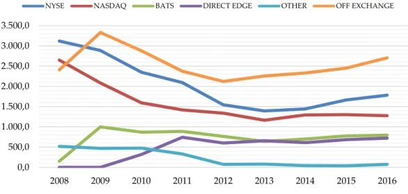
Figure 1 – Market Share Volume (Daily Avg., Mils. of Shares)

Source: Bats Global Markets

From the figure above, by examining the market share regarding daily average volume, we can verify that between 2009 and 2016 there was a decrease in the market share as a whole, most likely because of the most recent financial crisis (2007/2008). Further, we can observe that during this period, NYSE and NASDAQ had the most substantial decrease in market share. On the contrary, Direct EDGE had the most significant increase, reaching a stable market share since 2011. At the time, Bats has almost remained the same between 2009 and 2016. For last, we have the off-exchange market share, which since 2012 recovered its market power. By using only this figure, it would be hard to conclude anything, but we can attest that since 2008, the most significant exchanges (NYSE and NASDAQ), lost some market share to other exchanges.

1.2 Understanding Order Execution

Before analyzing the existing equity trading agents currently acting in U.S. equity markets, we need to understand how trades occur. Many studies review this process, so our effort in this subchapter is to give the fundamentals of this process without going too thick.

0,0 500,0 1.000,0 1.500,0 2.000,0 2.500,0 3.000,0 3.500,0 2008 2009 2010 2011 2012 2013 2014 2015 2016 NYSE NASDAQ BATS DIRECT EDGE OTHER OFF EXCHANGE

(21)

The trading process starts with a buyer or a seller trying to exchange its money for a stock, or vice-versa. Today, we can quickly start an account in an online trading platform, and send orders to the market without even thinking about the process behind the scene.

This process has been through some changes in the last few years, as a result of the internet boom (Choi, Laibson, & Metrick, 2002), and increasing regulation regarding market power, originating new financial intermediaries (Lee & Tierney, 2013), but essentials have remained the same.

Firstly, after an investor sends an order to buy or sell a stock on the market, the financial intermediary that receives the order – financial intermediary represents any entity that acts between parties, in this case between investors and trading venues – it will have to choose between different ways to fulfill the order. At this point, bear in mind the topic on regulation, regarding Order Protection Rule, which states that the financial intermediary has to choose the one that gives the investor the best price available in the market.

This best market price available can be relative, however. To choose to each trading venue to route the order, the financial intermediary has to choose the one that gives the best price having in consideration all costs that the investor can incur in a trade. These costs include explicit trading costs, for example, the fee paid to execute an order, and implicit trading cost, for instance, the opportunity costs regarding execute an order at time 𝑡, when compared to execute the same order at time 𝑡 + 1. We will discuss this subject later.

At this point, the financial intermediary has to choose between different options. First, it can attempt to fulfill the order on the trading floor, for instance, can send the order to be executed on the New York Stock Exchange (NYSE), or any other stock exchange. In the U.S. some exchanges with the intention of

(22)

22

Second, can place the order to a third market maker, this can occur in the U.S. by two reasons, the third market maker is giving an incentive to the financial intermediary lowering the cost or the financial intermediary may not can trade directly in that exchange. Financial intermediaries are required to be exchange members to trade securities in that exchanges directly.

Third, can internalize the order, matching buy-side orders with sell-side orders of investors within its portfolio, and since it would have to trade in any trading venue, can make some extra money on the charged spread.

Fourth, can use electronic communications network, matching buy and sell orders automatically, this case is usually used to limit order since this platforms can match these type of trades very quickly. And lastly, commonly used nowadays, can send the order to be executed over-the-counter by a market maker responsible for the security such as the NASDAQ.

Even though, the last option can be great for some institutional investors, investors that have the power to trade directly with these market makers. In some other cases, since these are less transparent markets, can lead to a moral hazard problem because trades can be routed to a market maker, just because is the one that pays the most significant fee to the financial intermediary – payment of order flow. Not giving the investor the best possible price available in the market, and making it the most unreliable orders in the investor perspective as the financial intermediary has the incentive to may not always send investor’s order to the best possible available price.

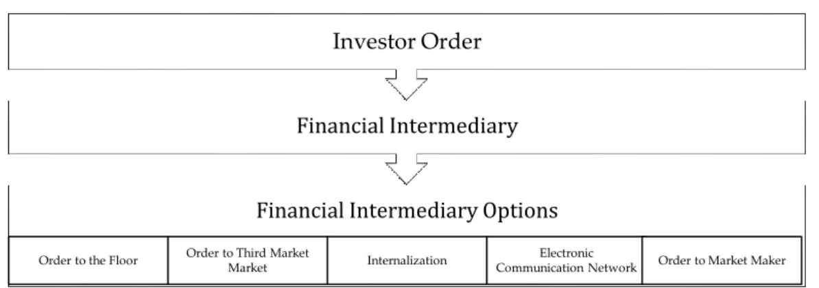
In the last stage, after the financial intermediary has chosen the option and sent the order to be executed, receives the details about the order execution and the custodian. A custodian is a financial institution that will safekeeping the securities to mitigate the risks related to theft or loss, charging a predetermined amount, which has to be in consideration when determining explicit trading costs. Figure 2 on the next page provides us a quick overview of this process.

(23)

Figure 2 – Understanding Order execution

1.3 Equity Trading Agents

In the previous subchapter, we saw that equity trading could occur on any of the public exchanges, Alternative Trading Systems (ATSs), Electronic Communication Networks (ECNs), or at off-exchange financial intermediaries, including internalization.

In respect of financial intermediaries, FINRA (Financial Industry Regulatory Authority (FINRA), a self-regulatory organization in charge of supervising financial intermediaries, over-the-counter markets, and some stock exchanges. Reported that as of December 2016, there was 3,835 registered ATSs, ECNs, or at off-exchange financial intermediaries firms, resulting in a decrease of 1,056 firms since 2008 (see Table 1).

Table 1 – FINRA Registered Financial Intermediaries

Year 2008 2009 2010 2011 2012 2013 2014 2015 2016

Total

Firms 4,891 4,718 4,578 4,457 4,29 4,146 4,068 3,943 3,835

Source: https://www.finra.org/newsroom/statistics

Financial Intermediary Options

Order to the Floor Order to Third Market _Market Internalization _{Communication Network}Electronic Order to Market Maker

Financial Intermediary Investor Order

(24)

24

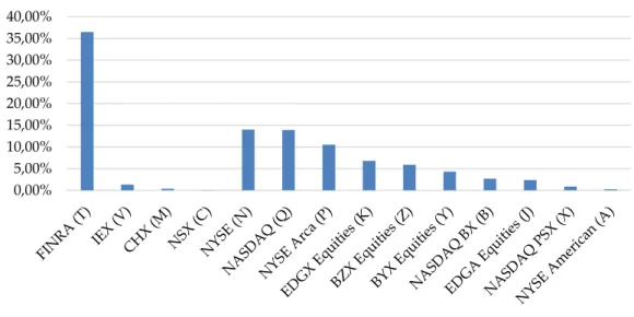
Figure 3 – Market Share (%) as of December 2016

Source: Bats Global Markets

Figure 3 shows us the market share (%), as of December 2016. We can perceive that most of the trading occurred in ATSs, ECNs, or at off-exchange financial intermediaries registered at FINRA, totalizing 36% of the trading, followed by NYSE and NASDAQ with 14% of market share for each, and NYSE Arca with 11%. Moreover, the remaining 25% of the market share, is distributed by all the others (IEX, CHX, NSX, EDGX Equities, BZX Equities, BYX Equities, NASDAQ BX, EDGA Equities, NASDAQ PSX, and NYSE American).

Moreover, Deutsche Bank reports that the share of high-frequency trading – automated trading programs using sophisticated algorithms to examine variables and markets, executing orders automatically reducing the execution time, hence, less implicit costs – accounts for approximately 40% of market volume in 2014 (Kaya, 2016). To a better understanding of the dramatic changes during recent years, as a result of increases in automation and entrance of new trading platforms see (Angel, Harris, & Spatt, 2011).

0,00% 5,00% 10,00% 15,00% 20,00% 25,00% 30,00% 35,00% 40,00%

(25)

Chapter 2 Theoretical Framework

2. Theoretical Framework

From the previous chapter we could understand that since the implementation of Reg NMS, and its Order Protection Rule, financial intermediaries, must best execute investors orders. Meaning that, if an investor wants to execute an order, the financial intermediary to comply with the law needs to route the order to the trading venue that minimizes investor costs.

This definition can be dubious, however. Financial intermediaries will have to take in consideration not only the fees and other cash payable costs that will be charged by the trading venue – explicit trading costs – but also, other intrinsic costs such us order execution time – implicit trading costs.

Furthermore, to study the competition between trading venues will be required to apply a unique trading demand model, as this model will need to capture and represent all the complexity of the trading execution process.

In this chapter we present a résumé of our main finding regarding the literature review, starting by examining the literature concerning trading costs, followed by the literature in-demand models.

(26)

26

2.1 Trading Costs Components

To accurately understand trading costs is essential to estimate the best possible order execution when dealing with to each trading venue to route investors order. This subchapter will present detail on this costs, as well as, give some insights about why the costs are so substantial when routing an order.

The literature typically splits these costs into two: explicit and implicit trading costs. The explicit trading costs related to all direct cash expenses that financial intermediaries can incur, such as the market fees. And the implicit trading costs related to the liquidity of a trading venue, such as the bid-ask spread (Brogaard, Hendershott, Hunt, & Ysusi, 2014; D’Hondt & Giraud, 2008; Keim & Madhavan, 1998; Ribeiro, 2010).

Moreover, these two costs are vitally connected to competition within financial markets by two main reasons. First, by increasing the competition, trading venues will have to lower their trading fees to be competitive, reducing its explicit costs. Second, the number of shares per trading venue in a competitive market is lower, diminishing the liquidity for each of them, hence, increasing the implicit costs of trading, e.g., larger bid-ask spreads, superior market impacts, and so forth (Bennett & Wei, 2006; Ribeiro, 2010). The next table presents the principal explicit and implicit trading costs that financial intermediaries have to consider regarding order execution.

Table 2 – Typology of Investors’ Trading Costs

Explicit Costs Implicit Costs

Brokerage Commissions Bid-Ask Spread

Market Fees Market Impact

Clearing and Settlement Costs Operational Opportunity Costs

Taxes/Stamp Duties Market Timing Opportunity Costs

Missed Trade Opportunity Costs

(27)

Even though, explicit trading costs are fundamental to estimate the execution costs we will not examine these costs deeply, since, to our research, we will apply a demand model regarding implicit trading costs. We only give a quick scope about each of these costs, followed by a comprehensive analysis of implicit trading costs.

2.1.1 Explicit Trading Costs

As from the last table explicit trading costs are related to all direct cash expenses, and can be divided into four central cash payments:

1. Brokerage commissions, the commissions paid to intermediaries for executing trades. Although this is a commission paid by investors to the financial intermediary, does not mean that the financial intermediary does not have to take this expense in consideration when trying to execute investors order at the best possible order execution. These costs vary from one intermediary to another, but they are a fixed and observable cost.

2. Market fees, the amount paid to exchanges for fulfilling orders. These fees are typically embedded into brokerage commissions and can vary from one trading venue to another, yet, higher volume markets usually have the lowest costs. As a result of competition, during the last years, it was observed a significant decrease in these costs (Gomber, Sagade, Theissen, Westheide, & Weber, 2017). Market fees are considered a fixed and observable cost.

3. Clearing and settlement costs are the amounts paid to transfer security rights permanently from one investor to another. These costs vary from

(28)

28

the one that the financial intermediary executed the order, yet, are considered fixed and observable costs.

4. Taxes/stamp duties are observable, but variable trading costs. They are observable as tax rates, or particular stamp duties known in advance but variable for the reason that they frequently differ by type of trade.

2.1.2 Implicit Trading Costs

In other words, implicit trading costs are characterized by its non-tangibility, representing the indirect costs such as the impact on the price occurred by trading some security, or the opportunity cost of not trading at some point in time, for instance, imagine the investor sent an order to the financial intermediary in period 𝑡1 went the stock was priced at $99, but could only be fulfilled in period

𝑡₂ when the price was already at $100, this represents a potential loss in value of $1.

In the extreme case, imagine that the financial intermediary could not fulfill the order at all. As a result, the investor had no explicit gains or losses. What these implicit costs tell us, though, is that actually, the investor had a potential gain or loss. If the order had been executed, the investor would have had a gain or loss - excluding the case that stock remains in the same price, having no losses or gain. However, even in this case could be argued that depending on the order size the market impact of this order could lead to changes in stock price, affecting the stock price upwards or downwards.

As we could understand from the previous example, these kinds of costs can be hard to estimate, and bring to the scientific community a whole new basket of question about how to best estimate these costs. Next, we presented the most used and accepted implicit trading costs measurements.

(29)

2.1.2.1 Quoted Bid-ask Spreads

Considered as the market maker’s return for providing liquidity. Represents the gap between the average price that investors are willing to pay and the average price that other investors are willing to sell a particular stock, resulting in more extensive spread lengths as liquidity decreases, early literature used this measure as a standard measure of implicit costs. Studies found that quoted spread in large market capitalization stocks (liquid stocks), when compared to small market capitalization stocks (illiquid stocks), can vary widely from 0.5% to 4-6%, respectively (Huang & Stoll, 1996).

Even though, this liquidity measure seems to be reliable, in fact, can result in incredibly inaccurate transaction costs and liquidity estimates. With a propensity to increase/decrease its length as a buy/sell trade occur, round turn transaction costs (all costs incurred in an order execution), might be less than quoted spreads suggests. Moreover, nowadays, trades can occur at prices outside the quoted bid or ask prices. For example, when a trade takes place over-the-counter, whereas a trade can occur at any price settled between two parties, this transaction will not be reflected on the quoted bid-ask spread (Keim & Madhavan, 1998).

2.1.2.2 Effective Bid-ask Spreads

To mitigate the issues regarding the quoted spreads, numerous authors have suggested measures. The effective bid-ask spread, however, firstly proposed by Roll (1984), and extended by George, Kaul, & Nimalendran (1991), and others, was the one that prevails. Being the most commonly used these days - even Reg NMS when it comes to disclosure of order execution information (Rule 605), require the market participants to disclose this measure.

(30)

30 Where we present its simpler version:

𝐸𝑓𝑓𝑒𝑐𝑡𝑖𝑣𝑒 𝑆𝑝𝑟𝑒𝑎𝑑_{𝐵𝑢𝑦−𝑠𝑖𝑑𝑒} = (𝑇𝑟𝑎𝑑𝑒 𝑃𝑟𝑖𝑐𝑒_𝑡− 𝑀𝑖𝑑𝑝𝑜𝑖𝑛𝑡_𝑡) ∗ 2

𝐸𝑓𝑓𝑒𝑐𝑡𝑖𝑣𝑒 𝑆𝑝𝑟𝑒𝑎𝑑_{𝑆𝑒𝑙𝑙−𝑠𝑖𝑑𝑒} = (𝑀𝑖𝑑𝑝𝑜𝑖𝑛𝑡_𝑡− 𝑇𝑟𝑎𝑑𝑒 𝑃𝑟𝑖𝑐𝑒_𝑡) ∗ 2

Where 𝑀𝑖𝑑𝑝𝑜𝑖𝑛𝑡𝑡 denotes the quoted bid-ask spread midpoint in period 𝑡, and

𝑇𝑟𝑎𝑑𝑒 𝑃𝑟𝑖𝑐𝑒_𝑡 the actual price at which the order was fulfilled in period 𝑡.

2.1.2.3 Market Impact

While the first two measures present us qualitative and quantitative measures for liquidity, neither of them compute possible trade price impacts for high volume trades.

When dealing with large orders, we have two effects that can occur and that will impact trade prices. The first effect, as equity markets nowadays are updated almost instantly, when large trades take place can influence other investors to buy or sell a stock, giving power to large traders to influence markets by merely putting a large order in place. Moreover, the second effect results from a trade large enough to surpass market maker willingness to trade, impacting the quoted price. For example, imagine a significant enough trade made by a sizeable institutional investor willing to buy a stock at $100, when a stock is quoting at $90. Probably, the stock will tend to $100 (Lakonishok, Shleifer, & Vishny, 1992). While theoretically simple, the price impact is hugely problematic when it comes to measuring because the price movement without the considering the order placement to the market is not observable.

Market impact measures are particularly relevant in the literature on block trades – usually considered to be above 10,000 shares or $200,000. For example, SUN & IBIKUNLE (2017) using high-frequency data from London Stock

(31)

Exchange (LSE), they found that the price impact of block trades is stronger during the first hour of trading.

2.1.2.4 Opportunity Costs

For last, we present the opportunity costs. Representing the most challenging measure of implicit trading costs because its assessment involves information regarding the exact moment that the trader decides to execute an order. The opportunity trading costs symbolize the costs of missed trades, more precisely lost in value resulting from the time between trade decision and execution. For instance, consider a trader that wants to execute a buy order in period 𝑡, since he believe that the stock price will go upwards, but he cannot fulfill its order. The cost of this missing trade can be measured by the difference between the price in period 𝑡, and the price in period 𝑡 + 1, resulting in a lost of value regarding this trade.

Three primary reasons drive these type of costs. First, an order can only be partially fulfilled or not fulfilled at all. Second, the price at which a trader desire to trade in 𝑡, can differ from the time at which the order is fulfilled 𝑡 + 1.

D’Hondt & Giraud (2008), show that three different opportunity costs can drive the time difference between the trade decision and the execution. Operational opportunity costs, for instance, the time required for financial intermediaries assess the best trading venue to where route the investor’s order. Market timing costs, for example, if an order is large enough, sometimes the financial intermediary needs to divide the order into small orders to minimize market impact, increasing the execution time. Finally, missed trade opportunity costs, represented in the first example, where the trader will have a loss in value since he could not fulfill the order, or could only fulfill it partially.

(32)

32

used the described approaches during this subchapter to measure implicit trading costs. Verifying that when executing an order it is imperative to consider all of them.

2.2 Financial Demand Models

To understand the applied model in this research, first, we need to comprehend that trading venues provide different trading services. Hence, we can view trading venues as differentiated products, in competition with each other throughout its basket of characteristics (Ribeiro, 2010). For example, if we remind the ways that a financial intermediary can route its orders, the Electronic Communication Networks were better when it comes to executing limit orders since these kinds of networks can match order much faster than any other trading venue. Thus, in this subchapter, we will focus on the literature in financial demand models applied to differentiated products.

2.2.1 Demand Models for Differentiated Products

The literature regarding trading demand models is scarce. Hence, in this subchapter, we will focus on the existing literature, directly and indirectly, connected to trading demand models. Presenting a quick overview of the literature on differentiated product models applied to financial systems as a whole.

Glaser, Rahman, Smith, & Chan(2013), using a panel data across seventy countries and seven years regarding the Microfinance Industry and applying a Bertrand model with a differentiated product, found that the increase in the number of Microfinance Institutions led to a remarkable increase in costumers’ welfare.

Hortaçsu & Syverson (2004), using a multinomial logit model to modeling the demand for mutual funds trading S&P 500 stocks. Found that regardless of

(33)

financial homogeneousness in what concerns this type of funds, still exists dispersion concerning the level of the fees charged by each fund, indicating that the fees charged are essential when it comes to mutual fund investors, but are not the only variable taken into consideration by investors.

Dick (2008), considering the U.S. bank branches as differentiated products, estimates a demand model using a nested logit model for commercial bank branch deposit services to evaluate the effects of the U.S. branching deregulation in the 1990s on depositors. Founding that the deposit rates and account fees are the primary drivers regarding this deposit decision and that depositors are favorable to the geographic expansion, resulting in a small upsurge in the welfare during the period analyzed.

Molnar, Nagy, & Horvath(2007), using a multinomial logit model and data on Hungarian commercial banks, estimate a demand model for deposit and loan services to study the market dominance in the Hungarian household credit and deposit markets. Founding that in the used sample period the competition in the Hungarian banking sector was low, resulting in high price-cost margins.

Ribeiro(2010), examine market dominance and barriers to competition regarding financial trading venues using a discrete-choice multinomial random-coefficient logit demand model. Founding that financial intermediaries have a tendency to value liquidity more than total fees when dealing with the order execution process.

To understand the theoretical model applied, first of all, we will need to retain from this subchapter that financial intermediaries have to choose to which trading venue to execute the investor’s order and that these trading venues differ from each other, competing through their varies characteristics.

(34)

34

Chapter 3 Theoretical Model and Econometric Strategy

3. Theoretical Model and Econometric Strategy

As we have seen before, trading venues provide different trading services, and the financial intermediary will have to choose the one best serves its interests. In this line, we can interpret the product offered by each trading venues as a product based on its differentiated basket of characteristics.

In this chapter, will be presented the theoretical demand model applied in our analysis as well as the econometric strategy used to analyze market dominance.

3.1 Theoretical Demand Model

When estimating a demand model for equity markets, different trading venues have different products which mean that we will have a dimensionality issue – with a large number of trading venues becomes unbearable to estimate the demand for each trading venue.

To deal with this issue, as other authors have done such as Dick (2008), Hortaçsu & Syverson(2004) and Ribeiro (2010), we use a multinomial logit model, becoming relevant only differences between characteristics of the differentiated product and not the number of trading venues.

For simplicity we will assume that in what concerns financial intermediaries, these agents will always choose the trading venue that maximizes investors’ utility – financial intermediaries are obligated by law to give each investor the best possible order execution.

(35)

This utility is dependent on two key factors. Intermediary characteristics, such as the payment for order flow (Battalio & Holden, 2001), and trading venues characteristics, such as the spreads or the execution time of a particular order (Ribeiro, 2010). Moreover, since financial intermediaries are the ones that choose each trading venue to route the investors’ orders, we assume that the utility function to investors equals the utility function to the chosen financial intermediary.

According to Berry(1994), this utility function splits into two distinct parts: the first part regarding specific features of trading venues, and the second one concerning specific characteristics of the financial intermediaries in charge to route investors’ orders.

The first part known as the specific features of the trading venue, which captures an average shared utility to all financial intermediaries, according to (Berry, 1994), is given by the following formula: 𝛿𝑗𝑎𝑡 = 𝑿𝑗𝑎𝑡𝜷 + 𝜉𝑗𝑎𝑡 (1), where

𝑿_𝑗𝑎𝑡 represents the observable characteristics vector of sending an order to a trading venue 𝑗 = 1, … , 𝐽, to execute an order on stock 𝑎 = 1, … , 𝐴, in period 𝑡 = 1, … , 𝑇 , such as effective spread; and 𝜉𝑗𝑎𝑡 represents the unobservable

characteristics of sending an order to a trading venue 𝑗 = 1, … , 𝐽, to buy/sell a stock 𝑎 = 1, … , 𝐴, in period 𝑡 = 1, … , 𝑇, such as explicit trading cost in our case.

The second part concerning specific characteristics of the financial intermediaries in charge to route investors’ orders, or in mathematical language, the individual deviation of each intermediary from the mean (1), is given by, 𝜀_{𝑗𝑎𝑖𝑡} (2), which can be read as the specific financial intermediaries characteristics to route investors’ orders to a trading venue 𝑗 = 1, … , 𝐽, to execute an order on stock 𝑎 = 1, … , 𝐴, by a financial intermediary 𝑖 = 1, … , 𝐼, in period 𝑡 = 1, … , 𝑇, for example the commission received to route trades to some trading venues.

(36)

36

𝑢_{𝑗𝑎𝑖𝑡} = 𝛿_𝑗𝑎𝑡 + 𝜀_{𝑗𝑎𝑖𝑡} = 𝑿_𝑗𝑎𝑡𝜷 + 𝜉_𝑗𝑎𝑡 + 𝜀_{𝑗𝑎𝑖𝑡} (3).

To fully understand order execution process in this model, i.e., financial intermediary’s options to where to execute the order, two concepts are essential and shall be distinguished.

Once the order is received, the financial intermediary has a basket of trading venues to where to route its trade. For our model, to compute the utility function as we will see afterward, we will need to exclude at least one from this basket of options resulting in two options. The inside option – trading venues considered in our model; and the outside option – trading venues considered in our model only for comparability.

In this line and since we are trying to compare between different trading venues, it is required to normalize the utility function, resulting in a normalized utility function for outside option, such that 𝛿0𝑎𝑡 = 0, which implies a utility

function 𝑢0𝑎𝑖𝑡 = 𝜀𝑗𝑎𝑖𝑡 (4), meaning that the utility function for the outside option

depends only on the specific characteristics of the financial intermediary, all else equal.

The specific characteristics of the financial intermediary leading to the choice of a particular trading venue be defined by:

(37)

where 𝐴𝑗𝑎𝑡 represents financial intermediaries choices to where to route

investors’ orders to a trading venue 𝑗 = 1, … , 𝐽, to execute an order on stock 𝑎 = 1, … , 𝐴, in period 𝑡 = 1, … , 𝑇; and 𝜹𝑎𝑡= (𝛿0𝑎𝑡, 𝛿1𝑎𝑡, … , 𝛿𝑗𝑎𝑡)

′

represents the vector of the average utilities associated with all platform 𝑗 = 0, … , 𝐽, to execute an order on stock 𝑎 = 1, … , 𝐴, in period 𝑡 = 1, … , 𝑇.

Given the latter equation, we can extract that the observed aggregate market share, 𝑆𝑗𝑎𝑡 of a given trading venue 𝑗 = 1, … , 𝐽, a stock 𝑎 = 1, … , 𝐴, in period 𝑡 =

1, … , 𝑇, will be given by the probability of vector 𝜀𝑗𝑎𝑖𝑡 be inside the region 𝐴𝑗𝑎𝑡:

𝑠_𝑗𝑎𝑡(𝜹) = ∫ 𝑑𝑃(𝜀_{𝑗𝑎𝑖𝑡})

𝐴𝑗𝑎𝑡

(6),

where 𝜀𝑗𝑎𝑖𝑡, the specific financial intermediaries characteristics to route investors’

orders to a trading venue 𝑗 = 1, … , 𝐽, to execute an order on stock 𝑎 = 1, … , 𝐴, by a financial intermediary 𝑖 = 1, … , 𝐼, in period 𝑡 = 1, … , 𝑇, which in consonance with Berry (1994), we considered to be independent and identically distributed (i.i.d.) of type I, extreme value distribution, making the non-linear aggregate market share of a given trading venue 𝑗 = 1, … , 𝑘, … , 𝐽, on a stock 𝑎 = 1, … , 𝐴, in period 𝑡 = 1, … , 𝑇, be given as:

𝑠_𝑗𝑎𝑡(𝜹_𝑎𝑡) = 𝑒 (𝛿𝑗𝑎𝑡) 𝑒(𝛿0𝑎𝑡)+ ∑𝐽 𝑒(𝛿𝑘𝑎𝑡) 𝑘=1 = 𝑒 (𝛿𝑗𝑎𝑡) 1 + ∑𝐽 𝑒(𝛿𝑘𝑎𝑡) 𝑘=1 (7),

Moreover, the demand elasticities associated with the observable characteristics vector, 𝑿𝜌𝑗𝑎𝑡, to a given financial intermediary characteristic 𝜌 =

(38)

38 𝜂𝑗𝑘𝑎𝑡 = 𝜕𝑠_𝑗𝑎𝑡 𝜕𝑋𝜌𝑗𝑎𝑡 𝑋_{𝜌𝑗𝑎𝑡} 𝑠𝑗𝑎𝑡 , 𝑤ℎ𝑒𝑟𝑒 { 𝛽𝜌 𝑋𝜌𝑗𝑎𝑡 (1 − 𝑠𝑗𝑎𝑡) 𝑖𝑓 𝑗 = 𝑘 −𝛽_𝜌 𝑋_{𝜌𝑗𝑎𝑡} 𝑠_𝑗𝑎𝑡 𝑜𝑡ℎ𝑒𝑟𝑤𝑖𝑠𝑒 (8).

3.2 Econometric Strategy

From the previous subchapter, we could see that the aggregate market share is a non-linear equation, and is dependent on the observable and unobservable characteristics of the existing trading venues in the market, making it complicated to estimate. Berry(1994), however, shows that it is possible to perform an estimation of this equation parameters using linear methods. Next, we will present the transformation process suggested, and that we used as well as a resource to estimate these parameters.

Consider 𝑆𝑗𝑎𝑡∗ as the observed market share to trading venue 𝑗 = 1, … , 𝐽, on a

stock 𝑎 = 1, … , 𝐴, in period 𝑡 = 1, … , 𝑇, and 𝑆𝑗𝑎𝑡 the market share resulting from

the model to trading venue 𝑗 = 1, … , 𝐽 , on a stock 𝑎 = 1, … , 𝐴 , in period 𝑡 = 1, … , 𝑇. Also consider 𝜹𝑎𝑡 as the vector of the average utilities to stock 𝑎 = 1, … , 𝐴,

in period 𝑡 = 1, … , 𝑇, such that, the estimated market shares by the model equal the observed market shares:

𝑠_𝑗𝑎𝑡(𝜹_𝑎𝑡) = 𝑆_𝑗𝑎𝑡∗ _(9),

Since 𝜹𝑎𝑡= (𝛿0𝑎𝑡, 𝛿1𝑎𝑡, … , 𝛿𝑗𝑎𝑡) ′

with 𝛿0𝑎𝑡 = 0, we are dealing with an equation

system with 𝐽 equations and 𝐽 unknown variables. Supposing that to all inside options equations 𝑗 = 1, … , 𝐽, exists a correlation between the estimated market shares and the observed market shares, we can also conclude that the same can be applied to the outside option, resulting in:

(39)

Similar rational can be applied to the market share equation (7), from the previous subchapter, so that the market share of the outside option will be given by: 𝑠_0𝑎𝑡(𝜹𝑎𝑡) = 𝑒(𝛿0𝑎𝑡) 1 + ∑𝐽 𝑒(𝛿𝑘𝑎𝑡) 𝑘=1 = 1 1 + ∑𝐽 𝑒(𝛿𝑘𝑎𝑡) 𝑘=1 (11),

By dividing both equations previously defined, (7) by (11),

𝑠𝑗𝑎𝑡(𝜹𝑎𝑡) 𝑠0𝑎𝑡(𝜹𝑎𝑡) = 𝑒(𝛿𝑗𝑎𝑡) 1 + ∑𝐽 𝑒(𝛿𝑘𝑎𝑡) 𝑘=1 1 1 + ∑𝐽 𝑒(𝛿𝑘𝑎𝑡) 𝑘=1 = 𝑒𝛿𝑗𝑎𝑡_(12),

Then, applying the logarithm to both sides, we obtain that:

𝑙𝑛 (𝑠𝑗𝑎𝑡(𝜹𝑎𝑡)

𝑠_0𝑎𝑡(𝜹_𝑎𝑡)) = 𝑙𝑛(𝑒

𝛿𝑗𝑎𝑡_{) = 𝛿}

𝑗𝑎𝑡 (13),

Finally, as 𝛿𝑗𝑎𝑡 = 𝑿𝑗𝑎𝑡𝜷 + 𝜉𝑗𝑎𝑡 (1), we can compute this equation as follow:

𝑙𝑛 (𝑠𝑗𝑎𝑡(𝜹𝑎𝑡) 𝑠_0𝑎𝑡(𝜹𝑎𝑡)

) = 𝑙𝑛(𝑆_𝑗𝑎𝑡∗ ) − 𝑙𝑛(𝑆_0𝑎𝑡∗ ) = 𝑿_𝑗𝑎𝑡𝜷 + 𝜉_𝑗𝑎𝑡 (14)

As a result, we have a linear model, where our dependent variable will be given by 𝑙𝑛(𝑆_𝑗𝑎𝑡∗ ) − 𝑙𝑛(𝑆_0𝑎𝑡∗ ), and represents the utility to execute the order into

(40)

40

the observed characteristic vector 𝑿𝑗𝑎𝑡 about trading venue 𝑗 = 1, … , 𝐽, stock 𝑎 =

1, … , 𝐴, in period 𝑡 = 1, … , 𝑇, and our unknown/unobserved variables will be in the error term 𝜉𝑗𝑎𝑡.

Lastly, since the data provided by trading venues regarding order execution, have limitations, not capturing all the relevant variables to our demand model, we used dummy variables as suggested in (Nevo, 2000). In our case, these variables can capture steady characteristics across trading venues, stocks or period, assuring that non-observable variables regarding order execution decision are in this dummies, reducing possible endogeneity issues.

(41)

Chapter 4 Empirical Analysis

4. Empirical Analysis

After a full scope, regarding order execution in the U.S. and literature regarding implicit costs of trading as well as demand models for differentiated products. In the chapter, we present the data description used to estimate the theoretical demand model along with the summary statistics and preliminary analysis, concluding with the results from estimation and price elasticities.

4.1 Data Description

Under the Rule 605 of the Reg NMS (formerly Rule 11Ac1-5), trading venues operating in the U.S. must make available specific order execution information monthly, facilitating the uniform public disclosure of order execution information by all market centers (https://www.sec.gov/reportspubs/investor-publications/investorpubsexqualityhtm.html).

We compiled this data across 13 exchanges and 59 alternative trading systems (ATSs) or over-the-counter (OTCs), FINRA members for the period between September 2016 and December 2017, resulting in a panel database. Table 3

(42)

42

Table 3 – Exchanges

BYX Equities IEX NASDAQ NYSE

BZX Equities CHX NASDAQ BX NYSE American

EDGA Equities NSX NASDAQ PSX NYSE Arca

EDGX Equities FINRA

This panel database provides us records about a set of execution-quality measures by trading venue, stock, period, order size, and order type, becoming enormous. To deal with this issue, in this thesis, we will only examine market orders and marketable limit orders for S&P 500 stocks during this period, accounting for 512 stocks. Moreover, we aggregated the estimation by orders size, considering small size orders, orders below 2000 shares, and large size orders, orders equal or above 2000 shares. Resulting in a much smaller sample (43,417 observations).

4.2 Model Variables

As already mentioned in the literature review, the financial intermediaries, when choosing the trading venue to place their orders, take into account several variables, such as the effective spread and the execution speed of execution of the financial. Since our data have limitations regarding the type of execution-quality measures, we had to adapt some of the existing variables in the data to estimate the demand model better. Resulting in three explanatory variables:

 The Avegare Effective Spread;

 The Weighted Average of Execution Time;

(43)

The average effective spread measures the total cost in dollars of executing an order. This measure computed by comparing the execution price of an order with the National Best Bid & Offer (NBBO) midpoint at the time the order is received:

𝐸𝑓𝑓𝑆𝑝𝑟𝑒𝑎𝑑𝐵𝑢𝑦−𝑠𝑖𝑑𝑒 = (𝑇𝑟𝑎𝑑𝑒 𝑃𝑟𝑖𝑐𝑒𝑡− 𝑀𝑖𝑑𝑝𝑜𝑖𝑛𝑡𝑡) ∗ 2

𝐸𝑓𝑓𝑆𝑝𝑟𝑒𝑎𝑑_{𝑆𝑒𝑙𝑙−𝑠𝑖𝑑𝑒} = (𝑀𝑖𝑑𝑝𝑜𝑖𝑛𝑡_𝑡− 𝑇𝑟𝑎𝑑𝑒 𝑃𝑟𝑖𝑐𝑒_𝑡) ∗ 2

Where 𝑀𝑖𝑑𝑝𝑜𝑖𝑛𝑡𝑡 denotes the NBBO quoted bid-ask spread midpoint in

period 𝑡, and 𝑇𝑟𝑎𝑑𝑒 𝑃𝑟𝑖𝑐𝑒𝑡 the actual price at which the order was fulfilled in

period 𝑡.

The weighted average of execution time is a variable adapted by us since such measure does not exist in the data. As the name indicates, respects to the average time to an order to be executed, after the placement to execute by the financial intermediary. Computed the by following formula:

𝑊𝐴𝐸𝑇 =

(𝐶𝐶𝑂𝐸0𝑠−9𝑠× 4,5) + (𝐶𝐶𝑂𝐸10𝑠−29𝑠× 19,5) + (𝐶𝐶𝑂𝐸30𝑠−59𝑠× 44,5) +

+ (𝐶𝐶𝑂𝐸60𝑠−299𝑠× 179,5) + (𝐶𝐶𝑂𝐸5𝑚−30𝑚× 1050)

𝑇𝐶𝐶𝑂𝐸

Where 𝐶𝐶𝑂𝐸0𝑠−9𝑠 denotes the cumulative covered orders executed between 0

and 9 seconds, 𝐶𝐶𝑂𝐸10𝑠−29𝑠 represents the cumulative covered orders executed

between 10 and 29 seconds, 𝐶𝐶𝑂𝐸30𝑠−59𝑠 indicates the cumulative covered orders

executed between 30 and 59 seconds, 𝐶𝐶𝑂𝐸60𝑠−299𝑠 denotes the cumulative

covered orders executed between 60 and 299 seconds, 𝐶𝐶𝑂𝐸5𝑚−30𝑚 represents

the cumulative covered orders executed between 5 and 30 minutes. For last, 𝑇𝐶𝐶𝑂𝐸 represents the total of all these cumulative covered orders, and the

(44)

44

The percentage of trades with price improvement, %𝑁𝑆𝑃𝐼, is also a measure adopted by us representing the percentage of trades that were fulfilled at higher/lower bid/ask price, than the quoted price at the time the order placed. Since our data give us the number cumulative covered orders executed with price improvement, and the total number of cumulative covered orders executed, we only need to divide the first by the second.

Regarding the market share (our dependent variable in the model), to compute this variable was necessary to define two new variables. One representing the total cumulative covered orders by platform, stock, and period, and another denoting the total cumulative covered orders only by stock and period. Once these two variables were defined, we could obtain the market share by dividing the first former by the latter.

4.3 Summary Statistics

Because financial intermediaries need to take in consideration the type and size of the order when deciding the trading venue to which they should route the order, we have divided the sample into four main types of orders. Type I - Market orders made by small investors, representing orders with a small size (<2,000 shares) to execute at the current market price. Type II - Market orders made by large investors, denoting orders with large size (=>2,000 shares) to execute at the current market price. Type III - Marketable limit order made by small investors, representing orders with a small size (<2,000 shares) to execute only if the stock reaches a certain price. Finally, Type IV - marketable limit order made by large investors, representing orders with a large size (=>2,000 shares) to execute only if the stock reaches a certain price.

Moreover, to mitigate risks regarding orders at abnormal prices, i.e., orders that would never fulfill we do not take into account in our model cancel orders.

(45)

Table 4 – Summary Statistics of Market Orders / Small Investors (I) *

Variables Mean Median Std. Dev. Min Max

𝐸𝑓𝑓𝑆𝑝𝑟𝑒𝑎𝑑 0.049740 0.023050 0.100141 -0.063450 4.031900

𝑊𝐴𝐸𝑇 4.840417 4.500000 1.503787 4.500000 57.582100

%𝑁𝑆𝑃𝐼 0.284777 0.174070 0.266631 0.000000 1.000000 𝑀𝑎𝑟𝑘𝑒𝑡 𝑆ℎ𝑎𝑟𝑒 0.231815 0.007522 0.364754 0.000011 0.465284

* The statistics presented are computed across 7,304 observations.

Table 4 presents statistics for the type I orders. From this measures we can observe the effective spread measured in dollars, was on average $0.05, the surpassing the double of the median value of $0.02, and having a standard deviation of $0.10. The weighted average execution time measured in seconds, was on average 4.84 seconds, outstanding the median value by 0,34 seconds, meaning that there were more orders executed in less time. The mean percentage of orders with price improvement measured was considerably higher that is median, 28.47%, and 17.41%, respectively. Meaning that, as expected, there exist more orders without price improvement. Regarding the market share, we can see that the market share for Type I orders seem to be a concentrated market, with trading venues counting for the majority of the market share since the average is much larger than the median, 23.18%, and 0.01%, respectively.

Note that since we only consider orders executed orders, the minimum value of the weighted average execution time is 4.5, i.e., the minimum that this variable can take.

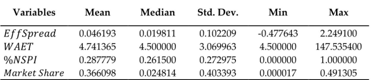
Table 5 – Summary Statistics of Market Orders / Large Investors (II) *

𝐸𝑓𝑓𝑆𝑝𝑟𝑒𝑎𝑑 0.046193 0.019811 0.102209 -0.477643 2.249100

𝑊𝐴𝐸𝑇 4.741365 4.500000 3.069963 4.500000 147.535400

(46)

46

Table 5 presents statistics for the type II orders. From this measures, we can observe the effective spread measured in dollars, behave in the same way as Type I orders, on average $0.05, the surpassing the double of the median value of $0.02, and having a standard deviation of $0.10. Regarding the weighted average execution time measured in seconds, was on average 4.84 seconds, also remaining higher than the median value but by 0,24 seconds, meaning that there were more orders executed in less time. The mean percentage of orders with price improvement measured was slightly higher that is median, 28.77%, and 26.15%, respectively. Lastly, concerning the market share, in Type II orders we can see that the market share orders seem to be also a concentrated market, with trading venues counting for the majority of the market share since the average market share is much larger than the median, 36.61%, and 0.03%, respectively.

Table 6 – Summary Statistics of Limit Orders / Small Investors (III) *

𝐸𝑓𝑓𝑆𝑝𝑟𝑒𝑎𝑑 0.043106 0.015200 0.130140 -0.006250 6,264200

𝑊𝐴𝐸𝑇 4.826642 4.508146 1.499632 4.500000 92.000000

%𝑁𝑆𝑃𝐼 0.023134 0.014615 0.032062 0.000000 0.4668683 𝑀𝑎𝑟𝑘𝑒𝑡 𝑆ℎ𝑎𝑟𝑒 0.067358 0.036308 0.093888 0.000001 0.5583832

Table 6 presents statistics for the type III orders. When it comes to marketable limit orders, the trading seems to be different from the market orders. We can observe the effective spread measured in dollars, behave in the same way as Type I and II orders, on average $0.04, the greater than the median value of $0.02, and having a standard deviation of $0.13. Regarding the weighted average execution time measured in seconds, was on average 4.83 seconds, also remaining higher than the median value by 0,31 seconds, meaning that there were more orders executed in less time. The mean as well as the median of the percentage of orders with price improvement, though, decreases significantly when compared to market order with values of 2.31%, and 1.46%, respectively. Probably driven by

(47)

the order type, since it only is executed if reaches a certain price, lowering the probability of price improvement orders. Moreover, concerning the market share in Type III orders, also the behavior in this market it is very different than in Type I and II. We can see from the market share that this is probably a fragmented market, with a large number of trading venues counting for the majority of the market share since the average market share is relatively low and slightly higher the median, 6.74%, and 3.63%, respectively.

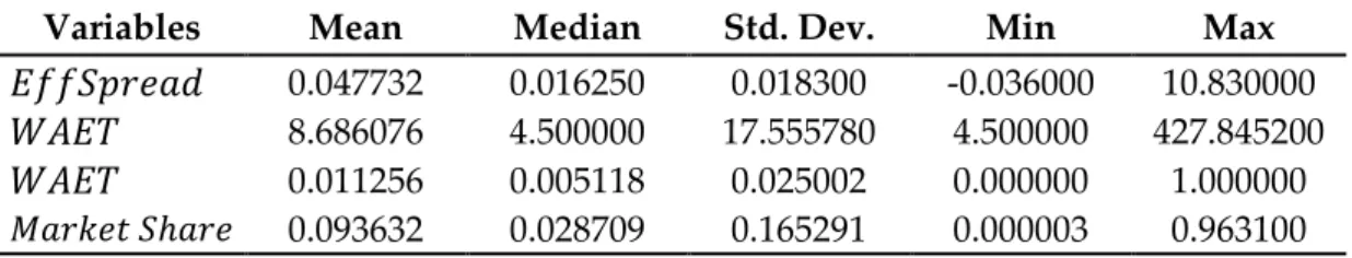
Table 7 – Summary Statistics of Limit Orders / Large Investors (IV) *

𝐸𝑓𝑓𝑆𝑝𝑟𝑒𝑎𝑑 0.047732 0.016250 0.018300 -0.036000 10.830000

𝑊𝐴𝐸𝑇 8.686076 4.500000 17.555780 4.500000 427.845200

𝑊𝐴𝐸𝑇 0.011256 0.005118 0.025002 0.000000 1.000000

𝑀𝑎𝑟𝑘𝑒𝑡 𝑆ℎ𝑎𝑟𝑒 0.093632 0.028709 0.165291 0.000003 0.963100

Table 7 presents statistics for the type IV orders. When it comes to marketable limit orders within large orders, the trading seems to be similar to marketable limit orders for small orders. We observe that the effective spread measured in dollars, behave in the same way as Type I, II and III orders, on average $0.05, the greater than the median value of $0.02, and having a standard deviation a little higher than in the other types of $0.18. Regarding the weighted average execution time measured in seconds, also a little higher than in the order types, on average 8.69 seconds, remaining higher than the median value 3,19 seconds, meaning that there were more orders executed in less time. The mean and median percentage of orders with price improvement also decreases significantly when compared to market order with values of 1.13%, and 0.01%, respectively. Finally, the market share, also the behaves in this market it is very different than in Type I and II. We

(48)

48

since the average market share is relatively low and slightly higher the median, 9.36%, and 2.87%, respectively.

4.4 Estimation and Price Elasticities Results

As we have seen before during the theoretical model chapter, we needed to create an outside option. To create the outside option we choose Bats Platforms as this option. Remain nine exchanges and FINRA, as inside options.

The next table presents the estimation coefficients as well as there level of significance for all the order’s type. Type I and II representing market orders for small and large investors, respectively. Type III and IV representing marketable limit orders for small and large investors, correspondingly.

Table 8 – Estimation Results * Specifications

Variables (I) (II) (III) (IV)

𝐸𝑓𝑓𝑆𝑝𝑟𝑒𝑎𝑑 -0.330507*** (0.090432) -0.278966** (0.155308) 0.335263*** (0.107916) 0.351561*** (0.096228) ln (𝑊𝐴𝐸𝑇) 0.026764 (0.051045) 0.080902 (0.087970) -0.226206*** (0.058368) 0.011972 (0.007297) %𝑁𝑆𝑃𝐼 0.124809*** (0.044512) 0.362875*** (0.093810) 1.609550*** (0.162943) -0.018422 (0.230126) R-Squared 35.89 16.07 15.87 14.71 Overall F-Test 194.23*** 39.91*** 94.92*** 29.71***

* All specifications include a constant term and dummy variables respect date and participant. Heteroskedasticity-robust standard errors clustered by security in parenthesis. *** denotes p-values <0.01, ** denotes p-values <0.05, and * denotes p-values <0.10.

By analyzing the specifications coefficients, we can state that across all the specifications the effective spread is significant at 1% level. However, contrary what we would expect, in the specifications III and IV, marketable limit orders, there is a positive relationship between the effective spread and the utility. Implying that as effective spread increase, the utility to execute orders in this trading venues also increase. We could not find research on this subject; however,

(49)

we can speculate that this may be caused by the payments for the order flow, since these payments incentivize financial intermediaries to trade in some trading venues, even though, the effective spread is higher than in other trading venues. Another explanation to this could be the fact that when dealing with marketable limit orders, financial intermediaries may choose the one that fastest matches its order to mitigate costs of missed trades.

Moreover, we can infer the only model where the weighted average execution time variable is significant at 1% level is on the model III, marketable limit order by small investors. This negative coefficient means that has execution time increases utility to route the order to these trading venues decreases. Corroborating the last statement regarding mitigating the costs of missed trades.

Finally, as expected, the percentage of the orders with price improvements has a positive and significant at 1% level relationships in three out of four models. Implying that as the number of orders with price improvements increase, the utility to send orders to these trading venues increase as well.

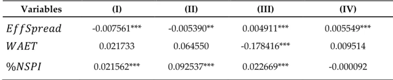
In what concerns the demand price elasticities, however, the scenario is different. From the next table we can extract that regarding the implicit trading costs variables considered in our model, although, some significant, we can see that still exists market dominance since all the elasticities derived from our model are inelastic.

Table 9 – Demand Elasticity Estimation by Variable

Variables (I) (II) (III) (IV)

𝐸𝑓𝑓𝑆𝑝𝑟𝑒𝑎𝑑 -0.007561*** -0.005390** 0.004911*** 0.005549***

𝑊𝐴𝐸𝑇 0.021733 0.064550 -0.178416*** 0.009514

(50)

50

Chapter 5 5. Conclusion

The Securities and Exchange Commission (SEC), driven by numerous studies regarding market competition and economic efficiency, recognizing these two variables as having a positive correlation (Casu & Girardone, 2009; Porter, 1990), started to implement policies against market dominance. On August 29th_{, 2005,} the Regulation National Markets System (Reg NMS) was released to harmonize regulation for equity trading services within the U.S., increasing competition and consumer protection in the trading industry services.

This research attempted to evaluate the effectiveness of Reg NMS regarding trading venues competition using a multinomial logit demand model for differentiated products with dummy variables to capture a non-observable variable.

After estimating the demand for the trading venues in the U.S. and analyzing its variables price elasticities (in our model we only considered implicit trading costs due to lack of data), from September 2016 to December 2016. Our findings suggest that, even though, implicit trading costs, are essential to estimate the trading demand still exists market dominance in the U.S. trading venues, resulting in unusually inelastic price elasticities. Further studies are required to understand the reason for such inelastic elasticities.

(51)

Bibliography

Angel, J. J., Harris, L. E., & Spatt, C. S. (2011). Equity Trading in the 21st Century.

Quarterly Journal of Finance, 5(1), 1392–1433.

Battalio, R., & Holden, C. W. (2001). A simple model of payment for order flow, internalization, and total trading cost. Journal of Financial Markets, 4(1), 33– 71. https://doi.org/10.1016/S1386-4181(00)00015-X

Bennett, P., & Wei, L. (2006). Market structure, fragmentation, and market quality. Journal of Financial Markets, 9(1), 49–78. https://doi.org/10.1016/j.finmar.2005.12.001

Berry, S. T. (1994). Estimating Discrete-Choice Models of Product Differentiation.

The RAND Journal of Economics, 25(2), 242. https://doi.org/10.2307/2555829

Bertimas, D., Lo, A. W., & Hummel, P. (1999). Optimal control of execution costs for portfolios. Computing in Science & Engineering, 1(6), 40–53. https://doi.org/10.1109/5992.805135

Brogaard, J., Hendershott, T., Hunt, S., & Ysusi, C. (2014). High-frequency trading and the execution costs of institutional investors. Financial Review,

49(2), 345–369.

Casu, B., & Girardone, C. (2009). Does competition lead to efficiency? The case of EU commercial banks. University of Essex Discussion Paper, 44(0), 1–35.

(52)

52

Evidence from investor behavior in 401(k) plans. Journal of Financial

Economics, 64(3), 397–421.

https://doi.org/https://doi.org/10.1016/S0304-405X(02)00130-7

D’Hondt, C., & Giraud, J.-R. (2008). Transaction Cost Analysis AZ: A Step towards

Best Execution in the Post-MiFID Landscape.

Davies, R., & Sirri, E. R. (2017). The economics and regulation of secondary trading markets. Working Paper, Columbia University.

Dick, A. A. (2008). Demand estimation and consumer welfare in the banking industry. Journal of Banking and Finance, 32(8), 1661–1676. https://doi.org/10.1016/j.jbankfin.2007.12.005

George, T. J., Kaul, G., & Nimalendran, M. (1991). Estimation of the bid-ask spread and its components: A new approach. Review of Financial Studies, 4(4), 623–656. https://doi.org/10.2307/2962152

Glaser, D. J., Rahman, A. S., Smith, K. A., & Chan, D. W. (2013). Product differentiation and consumer surplus in the microfinance industry. B.E.

Journal of Economic Analysis and Policy, 13(2), 991–1022.

https://doi.org/10.1515/bejeap-2012-0046

Gomber, P., Sagade, S., Theissen, E., Westheide, C., & Weber, M. C. (2017). Competition Between Equity Markets: A Review of the Consolidation Versus Fragmentation Debate. Journal of Economic Surveys, 31(3), 792–814.

(53)

COSTS, AND COMPETITION IN THE MUTUAL FUND INDUSTRY: A CASE STUDY OF S&P 500 INDEX FUNDS. The Quarterly Journal of

Economics, 119(2), 403–456.

Hu, G. (2009). Measures of implicit trading costs and buy-sell asymmetry. Journal

of Financial Markets, 12(3), 418–437.

https://doi.org/10.1016/j.finmar.2009.03.002

Huang, R. D., & Stoll, H. R. (1996). Dealer versus auction markets: A paired comparison of execution costs on NASDAQ and the NYSE. Journal of

Financial Economics, 41(3), 313–357.

https://doi.org/10.1016/0304-405X(95)00867-E

Kaya, O. (2016). High-frequency trading - Reaching the limits. Deutsche Bank

Research, 1–5. https://doi.org/10.1007/s13398-014-0173-7.2

Keim, D. B., & Madhavan, A. (1998). The cost of institutional equity trades.

Financial Analysts Journal, 54(4), 50–69.

Lakonishok, J., Shleifer, A., & Vishny, R. W. (1992). The impact of institutional trading on stock prices. Journal of Financial Economics, 32(1), 23–43. https://doi.org/10.1016/0304-405X(92)90023-Q

Lee, S., & Tierney, D. (2013). Market Fragmentation and Its Impact: a Historical

Analysis of Market Structure Evolution in the United States, Europe, and Canada.

The impact of implicit trading costs on trading venue competition