Envelope transient simulation of nonlinear electronic circuits using multi-rate Runge-Kutta algorithms

Envelope Transient Simulation of Nonlinear Electronic Circuits

Using Multi-Rate Runge-Kutta Algorithms

JORGE OLIVEIRA, ADÉRITO ARAÚJO* Department of Electrical Engineering

Technology and Management School - Polytechnic Institute of Leiria Morro do Lena, Alto Vieiro, Apartado 4163, 2411-901 Leiria

*Department of Mathematics University of Coimbra Apartado 3008, 3001-454 Coimbra

PORTUGAL

oliveira@estg.ipleiria.pt, alma@mat.uc.pt

Abstract: - Time-step integration is a popular technique commonly used for the envelope transient simulation of an electronic circuit. However, many kinds of circuits are characterized by widely separated time scales, which lead to significant computational costs when numerically solving its differential systems. Even so, this situation can be exploited in an efficient way using multi-rate methods, which integrate system components with different step sizes. In this paper two multi-rate Runge-Kutta schemes are studied and tested in terms of computational speed and numerical stability. The results for linear stability analysis here obtained are much more coherent with the characteristics of the methods than the ones previously presented in [6].

Key-Words: - Electronic circuit simulation, transient analysis, multi-rate Runge-Kutta methods, speed, stability.

1 Introduction

Transient analysis of an electronic circuit is usually expressed by an initial value problem of the form

( )

( )

( )

0 0

'

,

,

n

,

y t

=

f y

y t

=

y

y

∈R

t

>

t

₀

,

n

(1) where is the solution. This system of ordinary differential equations (ODEs) can be numerically solved by time-step integration, which is a classical technique that is commercially used by all SPICE like simulators. However, when integrating systems whose components evolve at different time scales one would like to use numerical methods that do not expend unnecessary work on slowly changing components. In such cases traditional time-step integrators become inefficient and numerical schemes with different time-step sizes are required. For example, in highly integrated electronic circuits normally only a small part of the elements is active, whereas the major part is latent. This latency can be exploited by multi-rate methods, which integrate components of the slow subsystem with a larger step length than the fast subsystem.

( )

t

y

Let us consider (1). If we split this ordinary differential system into active and latent subsystems we obtain

( )

(

)

( )

( )

(

)

( )

_{0 ,0} ' 0 , 0 '

,

,

,

,

L L L A L L A A L A A A

y

t

y

y

y

f

t

y

y

t

y

y

y

f

t

y

=

=

=

=

(2) with

,

A

,

L

,

A n n A L A L L

y

y

y

y

n

n

y

⎡ ⎤

=

_{⎢ ⎥}

∈

∈

+

⎣ ⎦

R

R

=

where _A is the active components vector and _L the latent components vector. The efficiency of the methods presented in this paper is verified only if there is a small number of fast changing components, i.e., if _A is a small subset of . It is so because while the active components _A are integrated with a small step size (microstep), the latent components

L are integrated with a large step size

y

y

y

y

y

h

y

H

(macro-step). The number of microsteps within a macrostep is

m

, thus

(

1/

)

,

.

h

=

m H

⋅

m

∈N

t_{0 h h h h …} t₀+ H H

Fig.1. Macro and microsteps

Throughout the integration process the partition into fast and slow components may vary with time, as well as . For a better understanding let us consider the basic example illustrated in Fig.2, where we have only five variables depending on t. Defining A as the active subsystem (fast changing components) and L

as the latent subsystem (slow changing components), then we will have

{

1

,

4

}

A

=

y y

,

L

=

{

y y y

₂

,

₃

,

₅

}

for t in the interval

[ ]

t t

₀

,

₁ and

{

2

,

5

}

A

=

y y

,

L

=

{

y y y

₁

,

₃

,

₄

}

for

t

∈

[ ]

t t

₁

,

₂ . t t₀ t₁ t₂ y1(t) y2(t) y3(t) y4(t) y5(t)

Fig.2. Active and latent components

2 Multi-Rate Runge-Kutta Methods

2.1 Definition

Let us consider two Runge-Kutta (RK) methods [5], [8], that can but do not have to be the same, expressed by their Butcher tableaus

(

b

,

A

,

c

)

and

(

b

,

A

,

c

)

, for integrating and , respectively. The resulting multi-rate Runge-Kutta (MRK) method

A

y

y

_L

for the numerical solution of (2) is defined as follows [6]:

• the active components

y

_A are given by

(

)

(

1

)

, 1 , , 1 , 0

∑

= + = + ≈ + + s i i A i A A A t h y y h bk y

λ

λ λ λ , 1 , , 1 , 0 − = … m

λ

,

,

2

,

1

,

~

,

_, , 1 , ,

f

y

h

a

k

Y

i

s

k

_{A j Li} s j ij A A i A

⎟⎟

=

…

⎠

⎞

⎜⎜

⎝

⎛

+

=

∑

= λ λ λ λ where

Y

Li

≈

y

L

(

t

+

(

λ

+

c

i

)

h

)

λ 0 ,

~

and

∑

, =

=

s j ij i

a

c

1

• the latent components

y

_L are given by

(

)

, 1 , 0 , 1 , 0

∑

= + = ≈ + s i i L i L L L t H y y H bk y

,

,

,

2

,

1

,

,

~

1 , 0 , , ,

f

Y

y

H

a

k

i

s

k

s j j L ij L i A L i L

⎟⎟

=

…

⎠

⎞

⎜⎜

⎝

⎛

+

=

∑

= where

Y

A,i

≈

y

A

(

t

0

+

c

i

H

)

~

and

∑

=

=

j ij i

a

c

1 s .

As we can see the coupling between active and latent subsystems is performed by the intermediate stage values

Y

A,i

~

and

Y

L,i

~

. There are several strategies for computing this values, like for example the ones suggested by Günther and Rentrop in [3] and [4], which are based in interpolation and/or extrapolation techniques. However, the algorithms studied and tested in this paper are the ones more recently proposed by Kværnø and Rentrop: MRKI and MRKII.

2.2 MRKI and MRKII Algorithms

In the MRKI algorithm the intermediate stage values

i A

Y

~

_, and

Y

~

_L,i are obtained by

( )

(

)

, ,0 1 j s L i L ij L j j

Y

y

h

γ

η λ

k

=

=

+

∑

+

_, 1, 2, , , 0,1, , 1, i= … s

λ

= … m− and 0 , ,0 , 1

,

1, 2,

,

s A i A ij A j j

Y

y

H

γ

k

i

=

=

+

∑

=

… .

s

We must note that the

Y

A,i

~

values are here somehow obtained by extrapolation from the first microstep. MRKII is a more robust algorithm, where the

Y

L,i

~

values are given just as in MRKI, but where the

Y

~

_A,i

values are obtained as follows: v₀ = y_A,0, k_L,1= f_L

(

y_A,0,y_L,0

)

for 1, 2,i= …,s−1 1

for ,

λ

=

c m

_i

…

,

c m

_i+

−

1

_{1 ,0}

( )

1

,

i A L ij L j

l

_λ+

f

v

_λ

y

h

ξ λ

k

=

⎛

⎞

=

_⎜

+

_⎟

⎝

∑

, j

⎠

v

_λ+1

=

v

_λ

+ ⋅

h l

_λ+1

end

1 , 1 ,0 1, 1 i c m A i A i

Y

y

H

_{λ λ}

l

λ

γ

+ + + =

=

+

∑

, 1 , 1 ,0 1, , 1

,

i L i L A i L i j L j j

k

₊

f

Y

₊

y

H

a

₊

k

=

⎛

⎞

=

_⎜

+

_⎟

⎝

∑

⎠

end

As we can see, in both MRK algorithms the

(

b

,

A

,

c

)

and

(

b

,

A

,

c

)

classical Runge-Kutta methods are connected by coupling coefficients. In the MRKI we have

γ

_ij,

γ

_ij and

η λ

_j

( )

, while in the MRKII we have

γ

_ij,

η λ

_j

( )

,

γ

_iλ and

ξ λ

_ij

( )

. Obviously all these coefficients must be carefully chosen, in way to guarantee a certain order, or to retain the order of the

(

b

,

A

,

c

)

and

(

b

,

A

,

c

)

, if they are of the same order. There are several ways to

derive order conditions for MRK methods, but the most appropriate seems to be rewriting them as partitioned Runge-Kutta (PRK) methods. By applying the already established order theory for PRK [5], order conditions for MRKI and MRKII may be found. All details of this order study can be seen in [7] or [9].

2.3 The Bogacki-Shampine RK Method

In both MRKI and MRKII algorithms described above we have considered for

(

b

,

A

,

c

)

and

(

b

,

A

,

c

)

the same method: the Bogacki-Shampine embedded Runge-Kutta method [1]. Its Butcher tableau is

0 0 1/2 1/2 0 3/4 0 3/4 0 1 2/9 3/9 4/9 0 i

b

2/9 3/9 4/9

ˆ

i

b

7/24 6/24 8/24 3/24 Table 1. Bogacki-Shampine (2)3

and it’s not difficult to verify that with

b

i this explicit

method is of order three, while with

b

ˆ

_i it is only of order two, in spite of having four stages (one extra stage is added for error estimation).

In this case one possible set of coupling coefficients that satisfies the order conditions up to three in MRKI and MRKII is presented in Table 2.

21 1 2 γ = ₃₁ 3

( )

1 1 4 m γ = − ₃₂ 3 4m γ =

(

)

2 1 1 3 1 2 4 2 m m m λ λ η = − + − −

(

)

2 2 1 3 3 1 2 4 2 m m m λ λ η = − + −

( )

2 3 1 1 2 m m λ λ η = − + 21 1 2 γ = ₃₁ 3 1( ) 4 m γ = − ₃₂ 3 4 m γ = 3 , / 2 5 4 m m γ = − _{3 , 3 / 4} 13 4 m m γ = _i, 1 m λ γ = ( ) ij i λ λ ξ =

Table 2. Coupling coefficients

We must observe that this choice of coupling coefficients is not unique. Other choices are possible. It is so because the number of coefficients is larger

than the number of order conditions (omitted here for brevity).

3 Stability

Numerical stability properties of various multi-rate schemes have been discussed by several authors. Unfortunately, most of these discussions (including the one presented in [6]) are not very detailed, nor very conclusive, and until now a concise theory is missing.

Beyond the study of the influence of the stiffness of the problem or the coupling between the active and latent subsystems, the main goal of this section is to compare the stability properties of MRKI with MRKII.

3.1 Multi-Rate Test Problem

The absolute stability properties of an integration method are usually studied by applying the method to the scalar test equation y'=

α

y, with

α

∈C−. Doing so for a standard Runge-Kutta method, the solution after one step is given by

h

( )

0

,

1

R

h

y

y

=

α

where

R

( )

h

α

is the stability function of the method. The method is stable if and only if

R

( )

h

α

<

1

[8]. However, multi-rate schemes require at least two components, so the linear differential system

' 11 12 2 2 ' 21 22

,

,

A A L L

y

y

y

y

α

α

α

α

×

⎡ ⎤

⎡ ⎤

⎡

⎤

=

=

∈

⎢ ⎥

⎢ ⎥

⎢

⎥

⎣ ⎦

⎣

⎦

⎣ ⎦

A

A

R

(3)

might be an appropriate test problem. If the assumptions

,

1

,

0

,

22 11 21 12 22 11

<

=

_α

_α

<

α

α

γ

α

α

are satisfied, then no extra conditions are required to ensure that both eigenvalues of have negative real parts. The parameter

A

γ

can be seen as a measure for the coupling between the equations and we also define

κ

=

α

₁₁

/

α

₂₂ as a measure for the stiffness of the system.

The numerical solution of (3) performed by the algorithms MRKI or MRKII after one compound step (1 macrostep H for _L and microsteps for

) can be expressed by

y

m

h

A

y

, , ,1 ,0

,

A m A L L

y

y

y

y

0

⎡

⎤

⎡

=

⎤

⎢

⎥

⎢

⎥

⎣

⎦

K

⎣

⎦

where

K

is a matrix that depends on H , , and the version of the MRK algorithm. It doesn't depend on the initial condition and for fixed step lengths

h A

and it remains constant throughout the integration

process.Thus, for example, from

h

0 1

y

=

y

K

11 ,0 12 ,0 , 21 ,0 22 ,0 ,1 A L A L

y

y

y

y

y

+

=

⎧

⎨

₊

₌

⎩

K

K

K

K

A m L

y

A m L

⎡

⎤

⎢

⎥

⎢

⎥

⎢

⎥

⎢

⎥

⎣

⎦

and

K

y

₁

=

y

₂ 11 , 12 ,1 ,2 21 , 22 ,1 ,2 A m L A m A m L L

y

y

y

y

y

y

+

=

⎧

⎨

₊

₌

⎩

K

K

K

K

we have 11 ,0 12 ,0 , 21 ,0 22 ,0 ,1 11 , 12 ,1 ,2 21 , 22 ,1 ,2

0 0

0 0

0 0

0 0

A L A L A m L A m A m L L

y

y

y

y

y

y

y

y

y

y

y

y

+

+ + =

⎧

⎪ + +

+

=

⎪

⎨

₊

_{+ + =}

⎪

⎪ + +

+

=

⎩

K

K

K

K

K

K

K

K

, that is to say, ,0 ,0 11 , ,0 ,0 12 ,1 , ,1 21 ,2 , ,1 22 ,2

0

0

0

0

0

0

0

0

A L A m A L L A m L A m A m L L

y

y

y

y

y

y

y

y

y

y

y

y

⎡

⎤ ⎡

⎤

⎢

⎥ ⎢

⎥

⎢

⎥ ⎢

_{⎥ =}

⎢

⎥ ⎢

⎥

⎢

⎥ ⎢

⎥

⎣

⎦

⎣

⎦

M

K

K

K

K

.

Now, if it is possible to find the entries

11, 12,

K

21 and 22. The method is stable if and

only if the spectral radius

( )

det

M

≠

0

K

K

K

( )

ρ

K

of the matrix satisfies .

K

( )

1

ρ

K

<

Step sizes

h

and H are chosen to ensure stability for the uncoupled system

(

α

₁₂

=

α

₂₁

=

0

)

, i.e., to ensure that the stability functions

R

_A

(

h

α

₁₁

)

and

(

H

α

22

)

R

_L satisfy the conditions

R

_A

(

h

α

₁₁

)

<

1

and

(

H

α

₂₂

)

<

1

R

_L . In the case of the

Bogacki-Shampine method that means [8] −2.54

<

h

α

₁₁

<

0 and −2.54

<

H

α

₂₂

<

0, that is to say,

H

<

2.54 and

κ

≥

m if, with no loss of generality, we make

1

22

=

−

α

. The question is to know how the coupling

γ

between the two systems affects the stability of the MRK and in what way it depends on

κ

, H and

m

.

3.2 Experimental

Results

Experimental results obtained computationally in

MATLAB® are shown in Fig.3, where we have plots

of some stability regions for , and

. The methods are stable below the boundaries and unstable above and as it can be seen these stability regions become smaller with increasing

1

κ

=

κ

=10 30

κ

=

κ

,

γ

and

m

. We have a o tested other values of ls

κ

larger than 30 and we obtained similar results with smaller regions (we just omitted them here for brevity). From the above we conclude that increasing the stiffness of the system, the coupling between the parts, or the number of microsteps, we force the methods to use a smaller macrostep H. We can also

see in Fig.3 that MRKII is more robust than MRKI, since it has larger stability regions. According to the performance of both algorithms, this result is more coherent than the one presented by Kværnø in [6].

4 Technical Details

erical results for the

.1 Stiffness

Detection

mbedded Runge-Kutta 1 1 ˆ i i i i i i i b b k h d k = = = Before presenting our num

simulation of an electronic test example with MRKI and MRKII, we will first introduce some technical details used for the code implementation of these two algorithms: stiffness detection, step size control and partitioning strategy.

4

The Bogacki-Shampine e

method used in both MRK algorithms is an explicit method. As we know, explicit codes applied to stiff problems are not very efficient. So, in order to avoid that MRKI and MRKII waste too much effort when encountering stiffness, it is important that the code be equipped with an automatic detecting stiffness structure. Our strategy is presented in the following. The local error of the Bogacki-Shampine method can be estimated by

4 4

err=h

∑

(

−

)

∑

. (4)

On the other hand, in a linear problem the numerical

where

solution after one step is given by

( )

1 0

y

=

R z y

,

( )

R z

is the stability function of the method

(

b

,

A

,

c

)

the same way we can say that

( )

1

ˆ

0

ˆy

=

R z y

, . In

with

R z

ˆ

( )

the stability funct n of the method io

(

b A

ˆ,

)

o, the error estimate can be given by

( )

( )

1

ˆ

1

ˆ

0

err

y

y

R z

R z

y

, c

. S

⎡

⎤

= − =

_⎣

−

_⎦

⋅

, that is to say,

( )

0

err

=

E z

⋅

y

, with

( )

( )

ˆ

(

E z

=

R z

−

R z

)

.

Let us consider now a new embedded Runge-Kutta method, replacing

b

ˆ

by

b

in the Bogacki-Shampine scheme. In a similar way, e have w

( )

( )

1 1

err=y −y =_⎣⎡R z −R z _⎦⎤⋅y₀,

i.e., a new error estimate defined by

( )

0

err

=

E z

⋅

y

, (5) with

( )

( )

( )

E z

=

R z

−

R z

.

The key idea is to choose the vector so that the method

(

is of order one, meaning that

b

)

→

, ,

b A c

( )

2 , when 0 err=O h h ,

and also that the condition

( )

( )

, 1

E z ≤

θ

E z

θ

<

is satisfied in the boundary of the stability region

ℜ

. If it is so, then we will have

err

err

for small

step sizes h, i.e., step sizes which are determined by accuracy requirements (when the problem is not stiff) and

err

<

err

when we are working near of the boundary of the stability region (the problem is possible stiff). A computer search gave us the following values for :

b

[

0.2817 0.2800 0.4353 0.0030

]

T

b

=

.

With theses values

E z

( ) ( )

E z

≈

0.3

in almost the whole boundary of

ℜ

, as we can see in Fig.4.

MRKI stable unstable unstable −1 −0.8 −0.6 −0.4 −0.2 0 0.2 0.4 0.6 0.8 1 0 0.5 1 1.5 2 2.5 γ H κ = 1 stable unstable unstable −1 −0.8 −0.6 −0.4 −0.2 0 0.2 0.4 0.6 0.8 1 0 0.5 1 1.5 2 2.5 γ H κ = 1 unstable unstable −1 −0.8 −0.6 −0.4 −0.2 0 0.2 0.4 0.6 0.8 1 0 0.5 1 1.5 2 2.5 γ H κ = 10 unstable unstable −1 −0.8 −0.6 −0.4 −0.2 0 0.2 0.4 0.6 0.8 1 0 0.5 1 1.5 2 2.5 γ H κ = 10

Fig.3. Stability regions: — m=8, --- m=12, ⋅-⋅ m=36, ⋅⋅⋅ m=100

−3 −2.5 −2 −1.5 −1 −0.5 0 0 0.5 1 1.5 2 2.5 4 2 1 0.5 0.25

Fig.4. Stability region ℜ and contour lines

( ) ( )

0.25, 0.5, 1, 2 and 4

E z E z =

4.2 Step

Size

Control

We want to have a code which automatically adjusts its step sizes in order to achieve a prescribed tolerance for the error. According to (4) the error estimates for the active and latent components in MRKI and MRKII algorithms are given by

4 , 1 , ,1 , 1 , A i A i L i err λ+ h d kλ err H d k = =

∑

= 4 1 i L i i=

∑

1

⎟

⎠

, (6) where

(

)

(

)

3 ,4 , 1 ,0 , 1

,

A A A L j L j j

k

λ

f

y

_λ+

y

h

η λ

k

=

⎛

⎞

=

_⎜

+

+

⎝

∑

and

(

)

,4 , , ,1 L L A m L k = f y y .

Selection of new step lengths h and H is performed at the end of each macrostep, and the whole strategy for automatic step size control throughout the numerical integration process goes as follows: based on the error estimates (6) a new step length hprop is proposed

for each component, defined by

1 1 0.8 p prop old

Tol

h

h

err

+

⎛

⎞

=

⋅

⎜

_⎜

⎟

_⎟

⋅

⎝

⎠

,

where Tol is the desired error tolerance, p is the order of the method and hold = h (active components) or

hold = H (latent components). The value 0.8 is just a

safety factor so that the error will be acceptable the next time with high probability. Additionally, alternative error estimates (5) are also computed for each component and if

err

<

err

the component is marked stiff. A new macrostep length Hnew is then

obtained by

min min

, 0.5 max

new prop prop

stiff all

H

h

⎛

⎛

⎞

⎛

⎞

⎞

⎜

⎜

⎟

_⎜

_⎟

=

⋅

⎜

⎜

⎟

⎜

_⎝

⎟

_⎠

⎝

⎠

⎝

h

⎟

⎟

⎠

,

but not allowed to increase too fast nor to decrease too fast,

0.5

⋅ ≤

H

H

_new

≤

1.5

⋅

H

,

to prevent a step size control with high zigzag. A new microstep length hnew is initially given by

min

new prop all

h

h

⎛

⎞

⎜

⎟

=

⎜

⎟

⎝

⎠

, and then the value of

new new

m

=

H

h

must be rounded to the nearest integer towards plus infinity (in MRKI), or to the nearest multiple of four towards plus infinity (in MRKII). The new microstep length hnew is finally found by

new new

h

=

H

m

.

4.3 Partitioning

Strategy

The partitioning of the differential system into the active and latent subsystems is done according to the following: each component that satisfies the condition _{prop new} will be treated as latent on the next iteration; the remaining ones will be treated as actives.

h ≥H

5 Sample Application

5.1 Electronic Pulse Generator

In order to test the performance and the efficiency of our multi-rate algorithms an electronic pulse gene-rator with MOSFETs was simulated with MRKI and MRKII. The schematic of this circuit is shown in Fig.5. R C VDD R C VDD vi v1 v2 R C VDD C R VDD vo vN

Fig.5. Pulse generator

This kind of circuit is commonly found in digital systems and it generates a positive pulse on its output when detects a transition from state 1 (high) to state 0

(low) on its input. It is constituted by an odd number of logical inverters connected in chain, followed by a NOR gate. The output of each inverter is the input of the next inverter and the charging and discharging of the capacitors produces delays in the run time of the signal. Thus,

v

_N is the logical negation of a phase shifted version of the input , and the output

v

_O is the logical NOR between

v

_i

and N. For a better understanding let us look at the

waveform chart illustrated in Fig.6. The input _i is a Heaviside (step) function where the transition from state 1 to 0 occurs at some time t. _N is also a step function, but due to the signal propagation delay the transition from one state to another occurs at some time . The result is a positive output pulse , in the interval

[

N

C

i

v

v

v

v

'

t

> t

v

O

]

, '

t t

. v_i v_O v_N 1 1 1 0 0 0 0 input voltage output voltage

Fig.6. Pulse generator waveform chart

5.2 Mathematical Model

Electronic circuit elements are characterized by equations which relate the voltage

v

across them to the current i through them (terminal voltage and current). In this case we have resistors R, whose terminal current and voltage are proportional

v i

R

= (Ohm’s law), capacitors

C

, which are characterized by

dv

i C

dt

=

and MOSFETs (metal oxide semiconductor field effect transistors). For these we chose a simple non dynamic model, a voltage controlled current source. Its characteristics are modeled in the following way:

0

GS GD

i

=

i

=

, G – gate, D – drain, S – source,

(

, ,

)

DS NL G D i = ⋅K g v v vS

))

))

0

S , where

g

_NL is a non linear function defined by

(

)

(

(

(

(

2 , 2

,

max

,

max

, 0

NL G D S G S T G D T

g

v v v

v

v

V

v

v

V

=

− −

−

−

−

with K = ⋅2 10−4AV-2 and

V

T

=

1

V.

The mathematical model of an electronic circuit (a network made up of interconnections of many circuit elements and generators) is based on Kirchhoff’s

current and voltage laws. Kirchhoff’s current law tells us that the net current into any node is zero. Kirchhoff’s voltage law says that the net sum of the voltage drops around any closed loop is zero.

Let us begin by applying the current law to node

1 (output of the first inverter) of the pulse generator.

We will have

v

R C D

i

= +

i

i

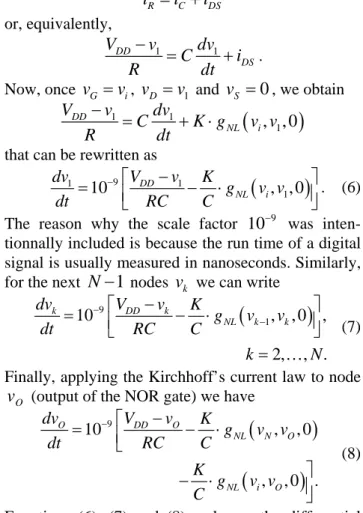
or, equivalently, 1 1 DD DS V v dv C i R dt − = + .

Now, once

v

_G

=

v

_i,

v

_D

=

v

₁ and

v

_S

=

0

, we obtain

(

)

1 1 1 , , 0 DD NL i V v dv C K g v v R dt − _{= + ⋅}

that can be rewritten as

(

9 1 1 1 10 DD , , 0 NL i dv V v K g v v dt RC C − ⎡ −

)

⎤ = _⎢ − ⋅ _⎥ ⎣ ⎦. (6)

The reason why the scale factor was

inten-tionnally included is because the run time of a digital signal is usually measured in nanoseconds. Similarly, for the next

9

10−

1

N

−

nodes

v

_k we can write

(

)

9 1 10 , , 0 , 2, , . k DD k NL k k dv V v K g v v dt RC C k N − − − ⎡ ⎤ = _⎢ − ⋅ _⎥ ⎣ ⎦ = … (7)

Finally, applying the Kirchhoff’s current law to node (output of the NOR gate) we have

O

v

(

)

(

)

9 10 , , 0 , , 0 O DD O NL N O NL i O dv V v K g v v dt RC C K g v v C − ⎡ − = − ⋅ ⎢⎣ ⎤ − ⋅ . ⎥⎦ (8)

Equations (6), (7) and (8) make up the differential system that models our pulse generator.

5.3 Numerical Simulation Results

The circuit with

N

=

51

inverters was simulated in

MATLAB® from

t

=

0

to ns, for an input

v

_i

transition at

40

=

t

1

=

t

ns. The numerical solution

v

O is

shown in Fig.7 and the overall results of this simulation are presented in Table 3. In all our tests we have considered VDD = 5V, R = 4.7 kΩ and

C= 0.2 pF.

time1 number of steps error in v_O

(sec) rejected macro micro ⋅ _∞ 2

L ⋅

MRKI 1.37 58 142 406 0.0048 0.0038

MRKII 2.15 60 135 616 0.0034 0.0029

Table 3. Numerical simulation results

1

Computation time (AMD Athlon 1.8 GHz, 256MB RAM).

In order to test the accuracy of the MRK methods a reference solution was achieved by numerically solving the ODE system (6)-(8) via classical time-step integration, using a classical Runge-Kutta method of higher order, with an extremely small time step. 0 5 10 15 20 25 30 35 40 0.5 1 1.5 2 2.5 3 3.5 4 4.5 5 t [ns]

Fig.7. Numerical solution

v

_O

6 Conclusions

After several simulation tests with different quantities of logical inverters and different integration intervals, we can say that in general both MRK methods show a good performance when solving our sample circuit. However, the MRKII algorithm leads to an increase of the computational work, once the total time for obtaining the numerical solution was in all cases bigger than in MRKI. In Section 3 we saw that the MRKII was a more stable method, nevertheless this stability gain implies a consequent loss of computa-tional speed. So, due to our opinion the MRKII algorithm must be chosen over MRKI only in stiff problems or when the coupling from the active to the latent part is strong.

References:

[1] P. Bogacki and L. Shampine, A (2)3 pair of Runge-Kutta formulas, Applied Math. Letters, No.2, 1989, pp. 1-9.

[2] M. Günther, A. Kværnø and P. Rentrop, Multirate partitioned Runge-Kutta methods, BIT, Vol.3, No.41, 2001, pp. 504-514.

[3] M. Günther and P. Rentrop, Multirate ROW methods and latency of electric circuits, Applied Numerical Mathematics, No.13, 1993, pp. 83-102. [4] M. Günther and P. Rentrop, Partitioning and

multirate strategies in latent electric circuits, International Series of Numerical Mathematics, No.117, 1994, pp. 33-60.

[5] E. Hairer, S. Nørsett and G. Wanner, Solving Ordinary Differential Equations I: Nonstiff Problems, Springer-Verlag, Berlin, 1987.

[6] A. Kværnø, Stability of multirate Runge-Kutta schemes, International Journal of Differential Equations and Applications, No.1A, 2000, pp. 97-105.

[7] A. Kværnø and P. Rentrop, Low order multirate Runge-Kutta methods in electric circuit

simulation, IWRMM Universität Karlsruhe,

Preprint No.99/1, 1999.

[8] J. Lambert, Numerical Methods for Ordinary Differential Systems: The Initial Value Problem, John Wiley & Sons, West Sussex, 1991.

[9] J. Oliveira, Métodos Multi-Ritmo na Análise e Simulação de Circuitos Electrónicos não Lineares, Master Thesis, Department of Mathematics, University of Coimbra, 2004.