Numerical Geometric Integration with HOMsPy
Asif Mushtaq
∗Abstract—The HOMsPy project is a collection of Python programs for some higher order geometric methods to solve a class of Hamilton equations numerically. The core program is thekimoki module, which uses symbolic algebra to generate a solver module for each specific Hamiltonian, together with a driver module example. Both double-precision and multi-precision modules can be generated. In this paper we (i) explain how to use the kimoki module with some illustrative well-known Hamiltonian problems, (ii) discuss how to run and modify the generated driver modules, and (iii) demonstrate through this some aspects of the implemented methods, like how well they respect energy conservation and time reversal invariance.
Index Terms—HOMsPy, higher-order-methods, symplecticity, automatic-code-generation, hamiltonians
I. INTRODUCTION
M
ANY fundamental problems in molecular dynamics, celestial mechanics, cosmology and in applied math-ematics can be modeled as Hamiltonian problems, providing a microscopic description of the particles (or similar ele-mentary subsystems) involved. To get insight into the often complicated behaviour of such models one must usually resort to numerical simulations. Hamiltonian systems arise at very large scales (celestial mechanics, cosmology) and at small scales (atoms and molecular simulations). The Hamilton equations of motion constitute a system of ordinary first order differential equations,˙
qa= ∂H
∂pa
, p˙a =−∂H
∂qa, a= 1, . . . ,N (1) where qa and p
a are generalized coordinates of positions and momenta, respectively, N is the number of variables, ˙ denotes differentiation with respect to time t, and H =
H(q,p). The initial conditions att= 0 can be written as,
qa(0) =qa0, pa(0) =pa0.
If we define,
z=
q p
,∇H =∂H
∂q1,· · · ,
∂H ∂qN,∂p∂H
1,· · ·,
∂H ∂pN
T
, (2)
the equivalent expression of (1) can be written as,
˙
z =J∇H, (3)
where
J =
0 Id
−Id 0
, (4)
is a skew-symmetric matrix. FurtherIdand0represent the (N × N) unit and zero matrices respectively. Hamiltonian problems usually belong to the class of ordinary differential equations which are difficult or mostly (almost) impossible
Manuscript received March 10, 2015; first revised June 05, 2015; second revised July 22, 2015
A. Mushtaq, Member IAENG, is with the Department of Mathematical Sciences, Norwegian University of Science and Technology, NTNU, N-7491 Trondheim, Norway. e-mail: [email protected].
to solve analytically. The equation of motion can be derived from the laws of physics for a physical system. Standard (traditional) numerical integrators which are used to simulate these equations, sometimes are not successful to provide the information about these (hidden) laws.
Several numerical approaches are implemented to find the solutions of Hamiltonian systems, but some of them are inappropriate for long-time simulations. In recent years geometric numerical integration methods are extensively used and gaining popularity for the solution of Hamiltonian problems. A geometrical integrator preserves one or more geometric (physical) property(ies) exactly (i.e. within the roundoff errors). In physical systems energy preservation, symmetries, time-reversal invariance, symplectic structure (for stochastic symplectic perspective we refer to [1]), an-gular momentum and phase-space volume are some very important and crucial geometric properties.
HOMsPy, Higher Order (symplectic) Methods in Python, is a collection of Python routines designed to generate nu-merical code for solving the differential equations generated by Hamiltonian of the form,
H(q,p) =1 2p
T
M−1p+V(q). (5)
The main goal of this program is to provide a framework for solving the Hamilton’s equations by some higher order symplectic algorithms proposed in [2], [3], using a symbolic program which automatically constructs the numerical solver, discussed in [4], for each specific Hamiltonian problem. The implemented symplectic schemes are based on extensions of the St¨ormer-Verlet method. Explicit implementation of the numerical code for a specific potential may be rather laborious and erroneous to do by hand, since repeated differ-entiation (with respect to many variables) and multiplication by lengthy expressions are often involved.
We have therefore written a code-generating program us-ing thesympysymbolic manipulation package. This takes a given potentialV as input, perform all the necessary algebra symbolically, and automatically writes a python module for solving one full timestep τ to the higher order (or selected order) of accuracy. The program also writes a runfile example (driver module) which demonstrates how the solver module can be used.
A. Important features of the program
Important aspects of this program are listed below:
• The program can handle Hamiltonian problems of the form
H(q,p)=T(p) +V(q),
whereT(p) = 1 2p
T
• The program has options for generating double-precision (DP) and/or multi-double-precision (MP) solver(s) for method(s) up to eight order in the timestep τ, and provides an automatic code generating environment.
• For a given Hamiltonian, a set of driver modules are automatically generated. In these, several parameters are given default values to this program. Further, initial values are generated randomly. It is straightforward for the user to change those.
B. Overview
The structure of the paper is following: In section II, general installation instructions for HOMsPy and associated packages are provided. Full automatic code generation of the program’s working is demonstrated on a simple pendulum problem in section III. In sections IV and V, mandatory and optional arguments of HOMsPy are discussed. In section VI, discussion on different aspects of the two degree of freedom problem Hamiltonian problem is presented with example code snippets. In section VII, some power of the multi-precision (MP) is demonstrated with the help of error analysis on a non-linear anharmonic oscillator. Time invariance reversibility is the part of section VIII and in section IX some concluding remarks are provided.
II. INSTALLATION AND CONFIGURATION
This program, as well as the generated solver and driver modules, is written in the Python programming language, using thesympy[5],numpy[6], and optionallympmath[7] libraries. In addition matplotlib[8] is used for plotting. In this section the focus of discussion will be the installation and configuration of necessary softwares as well as HOMsPy. For the basic understanding on scientific computations in Python and for general installation in detail, see [9].
A. Prerequisites
We have used Python version2.7.x, including the packages sympy,numpy,mpmath(for multi-precision calculations), andmatplotlibfor all development and testing. We have registered that incompatible combinations of these packages can lead to problems. We have not tested the code with Python version 3.x.
B. Installation of HOMsPy
• Download aesd_v1_0.tar.gz or later versions from
http://cpc.cs.qub.ac.uk/summaries/AESD v1 0.html, or ask the author for a copy of HOMSPy.tar.
• HOMsPy contains three subdirectories:
kimoki: The directory containing the code generating module.
examples:A directory containing a single file, named as
makeExamples.py. By running makeExamples.py eight new files will be generated, four solver modules (Vi-bratingBeam.py, AnharmonicOscillator.py, Anharmoni-cOscillatorMP.py, TwoDPendulumMP.py), and four run-file examples known as driver modules (runVibrating-Beam.py, runAnharmonicOscillator.py, runAnharmoni-cOscillatorMP.py, runTwoDPendulumMP.py). By run-ning each runfile example two .png plots will be
generated, <example> soln.png and <example>
EgyErr.png. Each runfile example will also generate several intermediate Python pickle (.pkl) files. These can normally be deleted after use.
demo: This directory demonstrates how the examples directory should look like after running makeExam-ples.py, and the runfile examples. Note that the figures will not look identical, because the examples are solved with random initial conditions. This directory in addi-tion contains six .log-files with output which is normally printed to screen. These files contains information about how long it takes to run the various programs.
C. Interactive use of the solver
The following simple interactive session will ensure the proper working of Python program and its associated pack-ages.
Interactive use of the solver module
1 >>> from __future__ import division 2 >>> from VibratingBeam import * 3 >>> z = numpy.array([1/3, 2/3]) 4 >>> kiMoKi(z); print z
5 [ 0.40155244 0.69839148] 6 >>> kiMoKi(z); print z 7 [ 0.47313122 0.73369218]
Herez = [q, p]is anumpyarray containing the current state of the solution. Each call ofkiMoKiupdates this state (data from previous time-steps are not kept).
III. USINGHOMSPY ON A SIMPLE PENDULUM Let us start with a simple illustrative example. Consider the pendulum problem defined by the Hamiltonian
H(q, p) =1 2p
2
−cos(q). (6)
The corresponding set of ODEs are
˙
q=p, p˙=−sin(q).
User can include the following code snippet in makeExam-ples.pyto get the solver as well as driver modules. One can opt the following procedure in oder to solve the pendulum problem by HOMsPy:
• First write a function specifying the Hamiltonian, giving symbolic names for the coordinates (q) and momentum (p) to be used (and optionally also additional parame-ters), and the symbolic expression of the potential V. In the present example there is just one coordinate and one momentum involved, with V =−cos(q). A code snippet for the pendulum problem is shown below, with the potential defined on line 7.
Creating a module for solving a pendulum problem
1 from sympy import cos 2 def makePendulum():
3 # Choose names for momentum
4 q, p = sympy.symbols([’q’,’p’]) 5 qvars = [q]; pvars = [p]
6 # Define the potential term
8 # Create code for DP solver
9 kimoki.makeModules(’Pendulum’, V, qvars, pvars)
Note that the sympy versions all the functions which occur in V must be known to the code generating program, since it must compute (higher order) symbolic derivatives ofV. This is why one has to import thecos -module from sympyin the snippet above.
Further, the numericalnumpyand/or mpmathversion of all these functions, and their generated derivatives, must be known to the solver module (with the same names as used by sympy). For this reason the solver module(s) always import most of the elementary func-tions (I.e., sqrt, log, exp, sin, cos, tan, sinh, cosh, tanh, asin, acos, atan, atan2, asinh, acosh, and atanh), using the appropriate names (see the top of Pendulum.py in this example). If more advanced functions (f.i. Bessel functions) are required, they must be added by hand to the imports at the top of the solver module.
• The call of
kimoki.makeModules(’Pendulum’,...) will generate a solver module, Pendulum.py, and runPendulum.pyas a demonstration driver module.
– Pendulum.py, the solver, contains all necessary code which is essential for our proposed higher or-der method. The user does not need to do anything with this file at the moment. But as an editable text file it is of course available for modification.
– runPendulum.py, an example driver module, is made to test the solver module, and provide a starting point for real applications. It provides solutions of the Hamilton equations for schemes of various orders, using random initial conditions and parameters, and generate plots of the results. The drivers modules are added in HOMsPy for the user convenience. They are ready to be executed, but user can easily be modified. This is sometimes even necessary.
In Figure 1, 8th order proposed method is used to solve the pendulum problem. Initial conditions are q(0) = 0 and p(0) = 1.0 with timestep
τ = 0.1. Here z0 denotes the position q, and z1
the momentump.
• One may now run the program runPendulum.py. Two separate tasks are executed by this program: First the subroutine plotSingelSolution() is called. This routine plots all components of a solution, generated with random initial values and parameters. The routine first checks if a solution has already been generated and saved to a pickle file, #Pendulum_SolnTau100Ord8.pkl. If the file does not exist, the subroutine computeSingleSolution(order) is called in order to generate a file with the solution. The solution is now read in and plotted, and the plot is saved to the file Pendulum_Soln.png; it will be similar to the plot in Figure 1.
NB!New execution of themakeExample.pycan be result in overwriting the existing driver module. Second the subroutine plotEnergyErrors() is
0 2 4 6 8 10 12 14 16
Time t
1.5 1.0 0.5 0.0 0.5 1.0 1.5
Solution
Numerical solution for timestep 1
10 and method of order 8 z0
z1
Fig. 1: Numerical solution of pendulum problem
called. This routine plots how well energy is preserved by the solver, for different values of the timestep τ
and order N of the solution. The energy error is expect to scale like τN with τ. The routine checks if#Pendulum_EgyErrTau<T>Ord<N>.pkl(with <T> = 500, 1000, and 2000, and <N> = 2, 4, 6, 8), has already been generated. If not, the subrou-tine computeEnergyErrors() is called in order to generate the required file(s), before the data is read in and plotted. The plots are saved to the file Pendulum_EgyErr.png. Figure 2 shows the scaled energy errors for different values of the timestepτ and orderN of the integrator. This figure verifies that the error scales like τN. The periodicity of the solution is reflected in the periodic variation of the energy error.
0 2 4 6 8 10 12 14 16 0.12
0.10 0.08 0.06 0.04 0.02 0.00 0.02 0.04
(E
(t
)−
E
(0)
)/τ
N
2nd order (
N =2)
0 2 4 6 8 10 12 14 16 0.005
0.000 0.005 0.010 0.015
0.020
4th order (
N =4)
τ =15
τ =1 10
τ =1 20
0 2 4 6 8 10 12 14 16 Time t
0.0060.005 0.0040.003 0.002 0.001 0.000 0.001
(E
(t
)−
E
(0)
)/τ
N
6th order (
N =6)
0 2 4 6 8 10 12 14 16 Time t
0.0005 0.0000 0.0005 0.0010 0.0015
0.0020
8th order (
N =8)
Approximate energy conservationFig. 2: Scaled energy errors forNth order methods.
• Some comments:
fine-tuning plots (which may require many iterations) from data taking long time to generate.
If the driver module crashes or is aborted, some pickle files (with names starting with the symbol #) may not have been removed.
For high-quality figures one may want to generate the plots in .pdf-format, with axes labels and legends by use of LATEX. This is possible in matplotlib, provided a working TEX-installation is detected. The driver module contains code for this (commented out to avoid unnecessary errors). In fact, most of the code in the driver module is related toplottingsolution and data, very little to generating it. A full routine to generate .pdf-format of Figure 2 is provided in appendix A.
IV. ARGUMENTS TO THE MODULE GENERATING ROUTINE
The main call in function in the module kimokiis
makeModules(’name’, V, qvars, pvars[, keywords]).
This will generate a solver and driver modules. The required arguments are listed in Table I.
TABLE I: Mandatory (positional) arguments
Name Description Symbols
’name’ basename of the generated file Pendulum Potential term potential term in term ofq V
Variables define necessary variables qvars, pvars
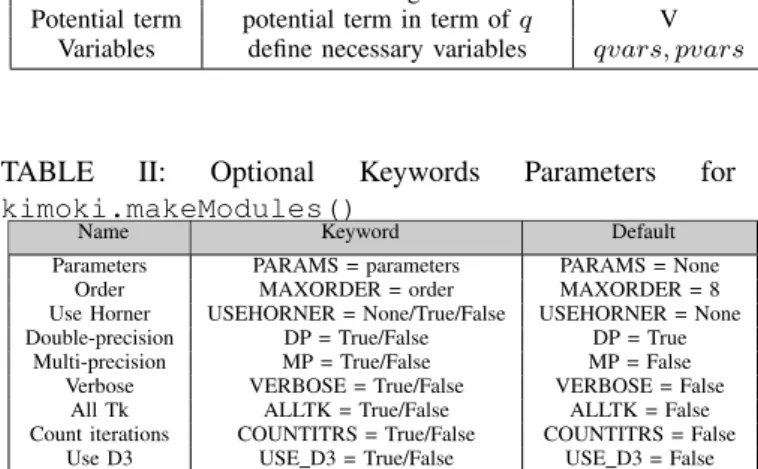
TABLE II: Optional Keywords Parameters for kimoki.makeModules()
Name Keyword Default
Parameters PARAMS = parameters PARAMS = None Order MAXORDER = order MAXORDER = 8 Use Horner USEHORNER = None/True/False USEHORNER = None Double-precision DP = True/False DP = True
Multi-precision MP = True/False MP = False Verbose VERBOSE = True/False VERBOSE = False
All Tk ALLTK = True/False ALLTK = False Count iterations COUNTITRS = True/False COUNTITRS = False
Use D3 USE D3 = True/False USE D3 = False
In addition a number of optional keyword arguments may be given. They are listed in Table II.Some explanations of the keyword parameters defined in Table II may be:
• The PARAMS keyword must be assigned a list of the symbolic parameters which occurs in the definition of the potential V. They can be used to make the solver module more general, but at the cost of longer and more complicated expressions in the numerical code.
• Thekimokimodule is capable of generating numerical solvers with accuracy up to orderτ8
, while the accuracy actually being used in each case is specified by a runtime parameter to the solver. There are cases where a solver of maximum order8is unwanted, because the code becomes too large and complicated, too slow to run, or takes too long to generate. For this reason there is a keyword argumentMAXORDER, which specifies the the maximum order of the generated code.
• For simple polynomial potentials it may be of some advantage to have expressions written in Horner or-dered form. There is a routine in sympy for making
such conversions. The parameterUSEHORNERspecifies whether it should be used. Given the valueNone it is used whenVis a polynomial in one variable, otherwise not; given the value True it is always used when V is a polynomial. It is our experience that the Horner conversion routine in sympy can be extremely slow and memory consuming.
• If the DP keyword is set to True double precision solver and driver modules will be generated. If the MPkeyword is set to Truemulti-precision solver and driver modules will be generated.
• When the VERBOSE keyword is set to True a fair amount of diagnostic messages about progress and time use is printed to standard output.
• Our higher order methods are based on generating an effective potential and effective kinetic energy
Veff(q) =V(q) +
3
X
k=1
Vk(q)τ2k, (7a)
Teff(q,p) = 12p
T p+
3
X
k=1
Tk(q,p)τ2k, (7b)
to be used in a St¨ormer-Verlet type integration scheme. However, the functionsTk(p,q)are not actually used in the integration scheme; instead a separately constructed generating function G(q,P;τ) is used. Hence, the functions Tk are not needed for the integrators. If the keyword ALLTK is set to True they are nevertheless generated.
• The integration steps which are based on the generating function (the pushsteps) G(q,P;τ)require numerical solution of a nonlinear algebraic equation. The solution of this is done by iteration, which seems to work well for small timestepsτ. To monitor the behavior of the iterative solver, the keywordCOUNTITRS may be set to True. This will generate code for constructing an histogram over the number of iterations. This his-togram is available as the array <name>.itrs. For the runPendulum example the number of iterations varies between 2 and 5.
• In the original proposal the potential V6 was defined in terms of an operator D3, cf. equations (32b) and (33) in ref. [2]. In ref. [4] it was realized that this is rather inefficient for problems with many variables, since the number of operations in D3 grows like N3.
An equivalent expression which is more efficient for largeN is given in footnote 4 on page 19 of ref. [4], and was implemented as default. The original version is used if the keywordUSE_D3is set toTrue; it may be slightly faster for small values ofN.
V. PARAMETERS OF THE SOLVER AND DRIVER MODULES A. Solver module parameters
The parameters available in the solver module are
we have used 10−12
for the double precision solvers, and10−20
for the multi-precision solvers (in the driver module examples these parameters have been changed to10−13and10−30respectively). Note that the
numer-ical precision used for the multi-precision solvers must be set in the driver module.
• The timestep used is defined by the parameter <name>.tau. By default tau is set to be 1
10 for
the double precision versions, and 1
100 for the
multi-precision versions.
• The order of integration to use is specified by the parameter <name>.order. It can be lower than the maximum order specified when the solver module was generated; the latter is available as the parameter <name>.maxorder(it is not good idea to change it).
• Other available parameters are <name>.params (a list of the potential parameters, possibly empty) and <name>.dim (the phasespace dimension 2N). They should not be changed either.
B. Driver module parameters
The driver module is likely to be modified according to use. The driver module parameters are,
• Initial valuesz0 are set to be random by default. These values can be model specific so user can easily change these values in the driver module. And nMax is the numeber of time-steps used to solve the system.
• Step-size τ is set to be 101 for double-precision
calcu-lation and 1
100 is set for multi-precision calculations.
VI. EXPERIMENTING WITHHOMSPY: HENON-HEILESHAMILTONIAN MODEL
In this section, a more interesting detailed interaction with HOMsPy will be demonstrated with some experimentation on the following Hamiltonian models. User can create his own deriver module. Our automatically generated deriver module is for the convenience and starting point for the user. The Henon-Heiles model is a Hamiltonian with two degree of freedom (N = 2). It is described in a classical paper of Henon and Heiles [11] in 1964.
The Hamiltonian is given by
H(q,p) = 1 2(kpk
2
+kqk2) +q2 1q2−q
3 2
3, (8) wherep= (p1, p2)andq= (q1, q2).
This test example will be used to demonstrate long-time energy conservation, potential motion, and Poincare’ section. An idea will be provided, how one can interact with HOMsPy to get more insight into the model problem. The solver and driver modules can be generated by the following code snippet which can be written inmakeExamples.py.
Creating a modules for solving Henon-Heiles model
1 def makeHenonHeiles():
2 # Choose names for coordinates
3 q1, q2, p1, p2 =
sympy.symbols([’q1’, ’q2’, ’p1’, ’p2’])
4 qvars = [q1, q2]; pvars = [p1, p2]
5 # Define the potential term
6 V = (q1**2 + q2**2)/2 + q1**2*q2 -q2**3/3
7 KiMoKi.makeModules(’HenonHeiles’, V, qvars, pvars)
Similar to earlier case, the call of
kimoki.makeModules(’HenonHeiles’,...) will generate a solver module, HenonHeiles.py, and a driver module, runHenonHeiles.py. At this point one can create its own driver module with the minimum lines of code provided in appendix B. But for demonstration and discussion, in subsections ahead, I will modify the driver module generated by the call of kimoki.makeModules(’HenonHeiles’,...). and will change the parameters involved in the model problem according to desire. I plug in initial values(0.12,0.12,− 0.12,0.12) and τ = 1
8 given in ref. [12] into the driver
module.
NB! The precautionary strategy is to change the name of driver module (runHenonHeiles.py) with an appropriate name like analyseHenon-Heiles.py. In this way one can escape of danger to overwrite the file in case of re-execution of themakeExamples.py
A. Long-time energy error
In Figure 3 engery errors are computed with Nth pro-posed methods. This figure shows the bounded energy errors for long time. A subroutine plotEnergyError() (see appendix C) is written in the driver module to generate Figure 3.
0 50 100 150 200 250
time t
10-17
10-16
10-15
10-14
10-13
10-12
10-11
10-10
10-9
10-8
10-7
10-6
10-5
10-4
E
(
t
)
−
E
(0)
N = 2
N = 4
N = 6
N = 8
Fig. 3: Computation of energy error with all proposed higher order symplectic methods by choosingτ = 0.125and initial values(q1, q2, p1, p2) = (0.12,0.12,0.12,0.12).
B. Motion in Henon-Heiles potential:
The potentialV(q)of this model basically has two kinds of behaviour with respect to motion, one is a regular motion and other one is a chaotic motion. These behaviors depend upon initial values and initial energies as discussed and showed in many numerical experiments in ref. [13]. For initial low energy the chaotic region is negligible. If the initial energy is less than 0.11 then the motion is regular and for initial energy 0.11 < E < 1
regular or chaotic depending upon the initial conditions. Figure 4 shows the surprising orbital motion at very low frequency generated my 8th order method. Choosing same parameters as in ref. [14], initial condition(q1, q2, p1, p2) = (0.025,0.050,0.0,0.0) , initial energy E0 = 0.0016, nMax =20000 andτ= 1. A code snippet is given in appendix D to plot Figure 4.
Fig. 4: Henon-Heiles potential motion by using 8th order proposed method.
C. Poincare’ section
Poincare’ section, also known surface to surface tech-nique, is a very efficient technique to visualize three dimen-sional constant energy trajectories.
This technique was introduced byHenri Poincare’ in the 20th century. Since the Henon-Heiles model has two degrees of freedom, we will use this technique. Detailed discussion on Poincare’ section is not our main aim but we will use it to show the performance of higher order methods. Without any loss of generality, fix the initial energy E0 and put q1= 0. Our aim is to plot (q2, p2), whenever the trajectory crosses the hyperplaneq1.
Further the fourth coordinatep1will depend upon the other three coordinates and fixed energy. The phase space is only bounded if the energy is less then 1
6 as discussed above.
For Poincare’ section considerE0as the initial fixed energy, defined as
H(q,p) =1 2(p
2 1+p
2 2) +
1 2(q
2 1+q
2 2) +q
2 1q2−1
3q
3 2 ≡E0
and initial condition
p1= r
2E0−p2 2−q
2 2+
2 3q
3 2.
The chaotic and non-chaotic behaviors of the motion by using the parameter used in ref. [12] are presented (for more details about Poincare’ map see [10]). Figure 5 shows the chaotic and non-chaotic motion of trajectories by using the 8thorder method. Left frame of this figure shows the regular motion of trajectories. We use (q2, p2) = (0.12,0.12),
τ = 1/6, initial energy E0 = 0.029952 , computed
p1 = 0.1796, and time-steps nMax = 1200000. Right frame of above figure is showing chaotic behaviour. We set
Fig. 5: Poincare’ section for the Henon-Heiles model.
q2 = p2 = 0, τ = 0.3, initial energy is E0 = 0.1592 , computed p1 = 0.5643 and time-steps nMax = 100000. ref. [12].
VII. MULTI-PRECISION(MP)VERSION OFHOMSPY In this section, I will present the second important aspect of our program by an illustrative example which we have discussed using double-precision (DP) version in ref. [4]. Higher order methods and multi-precision container solvers play very important rule to achieve high accuracy. Often some situations arise when minute information are required in many field of engineering, mathematics and physics. To tackle these situation multi-precision solvers can be impor-tant. In higher order accuracy for small values of time-steps rounding errors exceed the numerical truncation errors, multi-precision calculation is one of the way to fix this problem. In our paper [15], we discussed very-high-precision about the solutions of a class of Schr¨odinger type equations.
A. One parametric family of quartic anharmonic oscillator: procedural explanation
For the demonstration, we choose a problem of which the exact solution is known. In this example, we also demonstrate how parameter(s) (as α is a parameter given in equation (9)) can be included. Consider the non-linear anharmonic oscillator defined by the Hamiltonian
H= 1 2p
2
+α 2 q
2
+1 4q
4
Exact solution to this problem can be expressed in terms of the Jacobi elliptic functions [16],
q(t) =q0cn(νt|k), (10a)
p(t) =−q0νsn(νt|k)dn(νt|k). (10b)
Here the initial conditions are q(0) = q0, and p(0) = 0, which implies thatq0is either a maximum or a minimum of
q(t). The parameters and energy of the solution are given by
ν = α+q20
1/2
, k= 2−1/2q0/ν, E= α 2 q
2 0+
1 4q
4 0. (11)
For detailed description of this problem see ref. [4]. A code snippet to generating multi-precision solver and driver modules is the following:
Solving anharmonic oscillators with multi-precision (MP) strategy
1 def makeAnharmonicOscillator():
2 # Choose coordinate for momentum
3 q, p, alpha = sympy.symbols([’q’, ’p’, ’alpha’])
4 qvars = [q]; pvars = [p]; params = [alpha]
5 # Define the potential coordinate
6 V = alpha*q**2/2 + q**4/4
7 # Code for multiprec computations
8 kimoki.makeModules(’Anharmonic 9 Oscillator’, V, qvars, pvars, 10 DP= True, MP= True, VERBOSE= True)
The code in line 8 shows that the makeModules func-tion may take opfunc-tional inputs: If the MP keyword is set to True then two additional files are generated: In this case the files AnharmonicOscillatorMP.py, which is a solver module using multi-precision arithmetic, and runAnharmonicOscillatorMP.py, which is a driver module. When theVERBOSEkeyword is set toTruesome information from the code generating process will be written to screen, mainly information about the time used to process the various stages.
For further demonstration, I will consider theglobal error
at a fixed endpoint by using different time-steps. Here we have used the same parameter as discussed in [4]. In our driver module, we wrote the following routine:
Evaluation of the exact position and velocity of the initial value problem
1 def ze_(t, alpha, q0):
2 # Positive energy solution;
3 #q(t) varies between q0 and -q0.
4 if alpha + q0*q0/2 >= 0: 5 nu=numpy.sqrt(alpha + q0*q0) 6 k=q0/(nu*numpy.sqrt(2))
7 q=q0*mpmath.ellipfun(’cn’, nu*t, k=k) 8 p=-nu*q0*mpmath.ellipfun(’sn’,nu*t,k=k) 9 *mpmath.ellipfun(’dn’,nu*t,k=k)
10 return q, p
11 ze=numpy.vectorize(ze_)
In similar way, other two if-else conditions can be defined for the negative energy solutions where q(t) varies betweenq0 andq1 and also varies betweenq0 andq1> q0.
10−3 10−2 10−1 100
Timestepτ
10−25
10−23
10−21
10−19
10−17
10−15
10−13
10−11
10−9
k
(
q
(
t
)
,
p
(
t
))
−
(
qn
(
t
)
,
pn
(
t
))
k2
Global error at fix timet
DP MP Ref.line
Fig. 6: Convergence rates of double-precision (DP) and multi-precision (MP) solver by using8th order method at fix timet= 10. We usedτ = 1
10, 1 20,
1 40,
1 80,
1 160,
1
320,q0= 0.54
andα= 0.13.
Herezeis the exact solution written in vectorized form and ellipfun()is defined in mpmathfor the calculations of elliptic functions. In Figure 6, theL2 error is calculated by using DP and MP at fix timet. Atτ = 1
10 and 1
20, DP and
MP are behaving identically, at τ = 1
40 and afterwards DP
started to deviate and MP continues with the right behaviour (as expected). It is not due to failure of the8th order method but it is due to the limited accuracy of DP calculations. By increasing the accuracy till35 decimal places in MP, trend continues for very small time-stepsτ= 1
40, . . . , 1 320.
We may conclude that if one wants to use the full strength of higher order methods then the limits of double precision calculations must be superseded and opts for multi-precision calculations.
VIII. CHECK OF TIME REVERSAL INVARIANCE The equations generated by the Hamiltonian (5) is invari-ant under time reversal
T :t→ −t, q→q, p→ −p. (12)
I.e., if one
(i) starts with some initial conditionz0= (q(0),p(0)), (ii) integratesntimesteps forward in time to arrive at
zn= (q(nτ),p(nτ)), (iii) makes a time reversal
¯
z0= (q(nτ),−p(nτ))≡(q(0)¯ ,p(0))¯ , (iv) integratesnmore timesteps to arrive at
¯
zn= (q(¯nτ),p(¯nτ)), and
(v) finally makes a second time reversal, ¯¯
z0= (q(¯nτ),−p(¯nτ)),
one should be back at the start, z0 = ¯¯z0. This works well for the St¨ormer-Verlet method, which is explicitly time reversal invariant. One may check that in this case¯¯z0 andz0
only differs by an amount which depends on the numerical precision (about 15 decimals for standard double precision calculations), and not on the timestepτ.
one should expect z0¯¯ and z0 to differ by an amount which depends on the timestepτ and the order of the method.
This last example is an investigation of this feature for the pendulum problem discussed in section III. The solver module has already been generated, but we have to modify the driver module to the problem at hand. The basic steps for checking each case is
Code snippet for computation of solution with time reversal
1 soln0 = computeSolution(z0, tau, order, nMax)
2 z1 = numpy.array([soln0[-1][0], 3 -soln0[-1][1]])
4 soln1 = computeSolution(z1, tau, order, nMax)
5 z2 = numpy.array([soln1[-1][0], 6 -soln1[-1][1]])
7 # Closer starting point.
8 maxdiff = -1
9 for diff in z0-z2:
10 if mpmath.fabs(diff) > maxdiff: 11 maxdiff = mpmath.fabs(diff)
0 5k 10k 15k 20k 25k
10−15
10−14
10−13
10−12
10−11
10−10
10−9
10−8
10−7
10−6 Order = 4
0 5k 10k 15k 20k 25k
10−21
10−20
10−19
10−18
10−17
10−16
10−15
10−14
10−13
10−12
10−11
10−10
10−9 Order = 6
0 5k 10k 15k 20k 25k
10−27
10−26
10−25
10−24
10−23
10−22
10−21
10−20
10−19
10−18
10−17
10−16
10−15
10−14
10−13
10−12 Order = 8 Legend
τ= 1
10
τ= 1
20
τ=401
τ= 1
80
τ= 1
160
Approximate preservation of time reversal invariance
Fig. 7: This figure illustrates how well the solvers preserve time reversal invariance. We have used the same initial value
z0in all runs. As can be seen there is some weak dependence on the number of timesteps (ranging from 500 to 25 000). Further, the errors scales roughly like τN+2, where τ is
the timestep and N is the order of the method, with aN -dependent prefactor.
As shown in Figure 7 time reversal invariance is not preserved exactly, but to an accuracy which scales roughly likeτN+2, whereτis the timestep, andN is the order of the
method. There is a weak increasing trend with the number of timesteps. The methods preserve time reversal invariance to about the same accuracy as they preserve energy.
IX. CONCLUDING REMARKS
In this paper we have discussed the automatic genera-tion [4] of the higher order symplectic methods proposed by
Mushtaq et. al. [2]. To make the programs freely available to everyone, we have chosen to implement the automatic code generator in Python, using thesympypackage. This is not the best choice for complex problems; it is our experience that many sympy routines fail to scale well with problem size and complexity. Due to this problem we have not made any attempts to optimize the numerical code emitted by the code generator.
Further, the automatic code generator makes no attempts to find simplifying aspects of the problem, like underlying symmetries, or structured and/or linear behavior. For serious treatment of problems with such properties, it is the best to generate the codes directly from the expressions proposed in reference in [2].
For the generation of more efficient numerical codes, it is fairly straightforward to modifykimokito emit numerical code in other languages, like Fortran or C, amenable to further optimization by the compiler.
APPENDIX
A. Energy Errors of pendulum problem
Routine to plot the energy errors (Figure 2).
1 rc(’text’, usetex=True)
2 # Use this if you have LaTeX installed
3 import matplotlib; matplotlib.use(’PDF’) 4 def plotEnergyErrors():
5 subplots = [’221’, ’222’, ’223’, ’224’]
6 fig = pyplot.figure(1)
7 pyplot.subplots_adjust(wspace=0.4, hspace=0.25, top=0.9)
8 suptitle = r’Approximate energy conservation’
9 pyplot.suptitle(suptitle)
10 titles = [r’2nd order ($N=2$)’, r’4th order ($N=4$)’,
11 r’6th order ($N=6$)’,
r’8th order ($N=8$)’]
12 lines = [r’b’, r’r’, r’y’] 13 lws = [5, 2.5, 1]
14 xlabel = [’’, ’’, r’Time $t$’, r’Time $t$’]
15 for k in
xrange(PendulumMP.maxorder//2): 16 order = 2*k+2
17 fig.add_subplot(subplots[k]) 18 pyplot.title(titles[k]) 19 pyplot.xlabel(xlabel[k]) 20 if (k==0) or (k==2):
21 pyplot.ylabel(r’$(E(t) -E(0))/\tauˆN$’)
22 for ell in xrange(3):
23 # Read energy error from "pickle" file:
24 filename =
"#PendulumMP_EgyErrTau%dOrd%d.pkl" % (int(10000*taus[ell]),order)
25 try:
26 input = open(filename, ’rb’)
27 except:
29 computeEnergyErrors()
30 input = open(filename, ’rb’)
31 [tau, order, nMax,
energyError] = pickle.load(input)
32 input.close()
33 os.remove(filename) 34
pyplot.plot(tau*numpy.arange(nMax), energyError/tau**order,
35 lines[ell], lw=lws[ell], label=labels[ell])
36 if k==1:
37 leg =
pyplot.legend(loc=’upper center’) 38
leg.get_frame().set_alpha(0.65) 39 pyplot.savefig("PendulumMP_EgyErr",
dpi=1000, bbox_inches=’tight’) 40 pyplot.clf()
B. Driver module, created by user
Deriver module script which uses the solver module,
HenonHeiles.py
1 import HenonHeiles
2 HenonHeiles.tau = 1 3 HenonHeiles.order = 8 4 nMax = 20000
5 z0 =
numpy.array([0.025,0.05,0.0,0.0]) 6 soln = numpy.zeros((nMax,z0.size)) 7 energyError = numpy.zeros(nMax); 8 z = numpy.copy(z0);
9 soln[0,:] = z
10 energyError[0] = 0.0; 11 e0 = HenonHeiles.energy(z)
12 for n in xrange(1,nMax):
13 HenonHeiles.kiMoKi(z) 14 soln[n,:] = z
15 energyError[n] = HenonHeiles.energy(z)-e0; 16 times =
numpy.arange(nMax)*HenonHeiles.tau
C. Code snippet to produce energy errors
Solving Henon-Heiles model, with check of energy conser-vation
1 def plotEnergyError():
2 for ord in [2,4,6,8] :
3 z0 =
numpy.array([0.12,0.12,0.12,0.12]); 4 tau =0.125; nMax = 2001
5 err =
numpy.abs(computeEnergyError(z0, tau, ord, nMax))
6
pyplot.semilogy(tau*numpy.arange(nMax)
7 ,err)
8
pyplot.savefig("HenonHeiles_EgyErr")
Here the work of computing the energy error is been done at line 5. The function computeEnergyError is produced automatically, here we are just using it to fulfill our require-ment.savefig save the figure in pdf format. Figure 3 is the resulting output of this code snippet.
D. Code snippet for 3D representation Code snippet to plot Figure 4
1 fig = pyplot.figure()
2 ax = fig.gca(projection=’3d’) 3 ax.plot(deltaE1[:],
deltaE0[:],deltaE2[:],
’r.’,alpha=0.05, label =’N=8’) 4 ax.set_xlabel(r’$q_2$’),
ax.set_ylabel(r’$q_1$’), ax.set_zlabel(r’$p_1$’)
5 ax.legend(), ax.view_init(57, 18) 6
pyplot.savefig("HenonHeiles_MotionN8", dpi=1000, bbox_inches=’tight’)
ACKNOWLEDGEMENT
I would like to thanks prof. Anne Kværnø and prof. K˚are Olaussen for their useful discussions, helpful feedbacks, and careful proof reading of this document. I acknowledge sup-port provided by the prof. Trond Kvamsdal from department of mathematical sciences and also partial support provided by Statoil via prof. Roger Sollie, through a professor II grant in Applied mathematical physics.
REFERENCES
[1] L. Wang, J. Hong, and R. Scherer,”Stochastic Symplectic Approxima-tion for a Linear System with Additive Noises”, IAENG InternaApproxima-tional Journal of Applied Mathematics, vol. 42, no. 1, pp60-65, 2012. [2] A. Mushtaq, A. Kværnø, K. Olaussen, ”Higher order Geometric
Integrators for a class of Hamiltonian systems”, International Journal of Geometric Methods in Modern Physics, vol. 11, no. 1, pp1450009-1–1450009-20, 2014.
[3] A. Mushtaq, A. Kværnø, K. Olaussen,”Systematic Improvement of Splitting Methods for the Hamilton Equations”, Proceedings for the World Congress on Engineering, London July 4–6, vol I, pp247-251, 2012.
[4] A. Mushtaq, K. Olaussen, ”Automatic code generator for higher order integrators”, Computer Physics Communication, vol. 185, no. 5, pp1461-1472, 2014.
[5] SymPy Developement Team,http://sympy.org/
[6] NumPy Developers,http://numpy.org/
[7] F. Johanssonet. al.,”Python library for arbitrary–precision floating-point arithmetic”, http://code.google.code/p/mpmath/, 2010.
[8] J. D. Hunter,”Matplotlib: A 2D graphics environment”, Computing in Science & Engineering vol. 9, pp90–95, 2007
[9] C. F¨uhrer, J. E. Solem, O. Verdier, ”Computation with Python”, Pearson 2013.
[10] Q. Feng, ”Approximating Discrete Models for a Two-degree-of-freedom Friction System”, IAENG International Journal of Applied Mathematics, vol. 38, no. 1, pp1-8, 2008.
[11] M. Henon and C. Heiles,”The Application of the Third Integral of Motion: Some numerical experiments”, The Astronomical Journal, vol.69, no.1, pp69-79, February 1964.
[12] P. J. Channel, and J. C. Scovel,Symplectic integration of Hamiltonian systems, Nonlinearity 3, pp231–259, 1990
[13] G. Benettin, L. Galgani, J. Strelcun,”Kolmogorov entropy and numer-ical experiments”, Physnumer-ical Review A, vol. 6, pp2338–2345,1976. [14] R. I. McLachlan, and G. R. W. Quispel.”Geometric integrators for
ODEs”, Journal of Physics A: Mathematical and General, vol. 39, no. 19, pp5251-5281, 2006.
[15] A. Mushtaq, A. Noreen, K. Olaussen, I. Øverbø,”Very-high-precision solutions of a class of Schr¨odinger type equations”, Computer Physics Communications, vol. 182, no. 9, pp1810-1813, 2011