M ASTER IN A CTUARIALS CIENCE M ASTER ´SF

(1)

M

ASTER IN

A

CTUARIAL

S

CIENCE

M

ASTER

´

S

F

INAL

W

ORK

T

HESIS

A

S

TUDY ON

T

HIELE

’

S

D

IFFERENTIAL

E

QUATION

A

LICE

L

OUREIRO

L

EOCÁDIO

B

OTELHO DE

L

EMOS

(2)

2

M

ASTER IN

A

CTUARIAL

S

CIENCE

M

ASTER

´

S

F

INAL

W

ORK

T

HESIS

A

S

TUDY ON

T

HIELE

’

S

D

IFFERENTIAL

E

QUATION

A

LICE

L

OUREIRO

L

EOCÁDIO

B

OTELHO DE

L

EMOS

Supervisor: Prof. Onofre Alves Simões

(3)

3

Alice Loureiro Leocádio Botelho de Lemos

Master in Actuarial Science

Supervisor: Onofre Alves Simões

Abstract

Thiele's differential equation has a long history, dating back to an unpublished note of Thiele, 1875 (Gram, 1910). Thorvald Nicolai Thiele was a Danish researcher who worked as an actuary, astronomer, mathematician and statistician. He proved that for a whole life assurance of a single individual with benefit of amount 1, payable immediately on death, the prospective reserve satisfies a certain linear differential equation, which is extremely useful for the understanding of reality: Thiele's differential equation. In a more general framework, Thiele's differential equations for the prospective reserve are a linear system of differential equations describing the dynamics of reserves in life and pension insurance in continuous time.

This text has the main purpose of reviewing in a comprehensive way the contributions related to Thiele’s equation that appeared over time, presenting the status of the art on this important topic. A revision of life insurance mathematics is first given (Dickson et al. 2013; Bowers et al.1997) and then Thiele’s differential equation is derived under the classical and multiple state model of human mortality for one life and for multiple lives (Hoem 1969). After this, some illustrations are presented under different types of contracts. Following the developments in the literature, more general differential equations are obtained, including a stochastic payment process (Norberg 1992a and Møller 1993) and a diffusion process for interest rate (Norberg and Møller 1996). The technique of using Thiele’s differential equation as a tool for life insurance product development (Ramlau-Hansen 1990 and Norberg 1992b) and the generalization of the equation for a closed insurance portfolio (Linnemann 1993) are also discussed. Finally, other developments are summarised (Milbrodt and Starke 1997, Steffensen 2000, Norberg 2001 and Christiansen 2008 and 2010).

(4)

4

Alice Loureiro Leocádio Botelho de Lemos

Mestrado em Ciências Actuariais

Orientador: Onofre Alves Simões

Resumo

Thorvald Nicolai Thiele foi um importante investigador dinamarquês, que trabalhou como atuário, astrónomo, matemático e estatístico (Gram, 1910). Entre os seus contributos, destaca-se em particular o facto de ter provado que para um seguro de vida inteira com benefício de valor 1, emitido sobre uma pessoa e pago imediatamente após a morte, as reservas prospetivas satisfazem uma equação diferencial linear que veio a revelar-se de grande importância para a compreensão do processo de formação das reservas: a chamada equação diferencial de Thiele. De um modo mais geral, as equações diferenciais de Thiele, para as reservas prospetivas, são um sistema diferencial linear de equações que descrevem a dinâmica das reservas nos seguros de vida e pensões em tempo contínuo.

Este texto tem como principal objetivo rever de forma tão completa quanto possível as contribuições relacionadas com a equação de Thiele que foram surgindo ao longo do tempo, dando assim ‘the present state of the art’deste relevante tópico. Começando por fazer uma revisão breve do essencial da matemática atuarial (Dickson et al.2013; Bowers et al.1997), avança depois para a derivação da equação de Thiele, considerando os dois modelos de mortalidade, o clássico e o de múltiplos estados, sobre uma pessoa e sobre várias pessoas (Hoem 1969). Algumas ilustrações, para vários tipos de contrato, são seguidamente introduzidas. Dos desenvolvimentos conhecidos, dá-se especial destaque às generalizações da equação diferencial que incluem um processo estocástico de pagamentos (Norberg 1992a e Møller 1993) e um processo de difusão para a taxa de juro (Norberg e Møller 1996). Apresenta-se também o uso da equação como ferramenta para o desenvolvimento de produtos de seguro de vida (Ramlau-Hansen 1990 e Norberg 1992b) e descreve-se uma generalização da equação diferencial para uma carteira fechada de seguros (Linnemann 1993). A última parte do trabalho faz um resumo de outros contributos relacionados com a equação (Milbrodt e Starke 1997, Steffensen 2000, Norberg 2001 e Christiansen 2008 e 2010).

(5)

5

Acknowledgements

First, I would like to thank Professor Onofre Alves Simões for the important and valuable suggestions given throughout the term to write this dissertation. Then, I am also grateful to all Professors of the Master’s courses for their insightful lectures.

(6)

6

LIST OF TABLES

TABLE I - Valuation of a life contingent single benefit of amount 1 in continuous time………..…16 TABLE II - Valuation of a life contingent single benefit of amount 1 in discrete

time ……….17

TABLE III - Valuation of life contingent annuities ………..….17

LIST OF FIGURES

(9)

9

«INSURANCE – the pooling of risk helps us to lead more predictable lives. The ability to insure assumes that there is some technology capable of calculating large and complex risks, and some organizational form that can mobilize the financial resources to underwrite the calculations (…). The second half of the eighteenth century was a time of major innovations. One of the big innovations concerned life insurance. Unlike practically every other branch of insurance, it was a European invention (…). »

(10)

10

1. Introduction

Over the last two centuries life insurance theory has evolved significantly. The advance of computers has contributed to apply models and develop new products in an unprecedented way. Nowadays actuaries are able to build highly sophisticated models with powerful software to manage risks arising from insurance business.

Actuarial theory is of crucial importance for insurance business to remain solvent and to satisfy all parties of the business: shareholders, stakeholders and policyholders. The contribution of early actuaries and mathematicians to actuarial theory is of unquestionable importance. During the last century many actuaries have studied and applied early theory and contributed to new findings and new theories.

One of the earliest actuaries and a most influential scientist of his time was Thorvald Nicolai Thiele. He was born in 1838 in Denmark and was astronomer, mathematician, statistician and actuarial mathematician. Among the many contributions he made to the advance of knowledge there is a significant work in the field of actuarial theory. In particular and more important in the framework of this dissertation is the fact that his name is associated with a differential equation that will be introduced later on: Thiele’s

differential equation (TDE) (Lauritzen 2002).

TDE is a powerful and insightful equation that has many applications in insurance mathematics and actuarial practice. This equation was only published in Thiele obituary by Gram in 1910.

(11)

11

(12)

12

2. Life Insurance

2.1 Life insurance contracts

An insurance contract is a written agreement under which one party, the insurer, accepts a risk from another party, the policyholder, by agreeing to pay a compensation (called the benefit) if the specified uncertain future event occurs, in exchange for a premium paid by the policyholder.

Life insurance contracts cover mortality and longevity risks as well as savings. They are usually long term contracts where the benefit is commonly known at outset. Non-life insurance contracts cover a multitude of natural and man-made perils. They are usually short term coverage and the benefit is commonly unknown.

(13)

13

2.2 Technical bases

The projection of future cash flows under a life insurance contract for pricing and valuation purposes give rise to the need of derivation and development of actuarial assumptions, called the actuarial bases or technical bases. Actuarial assumptions have to be considered regarding future interest rates to discount cash flows to the present, future rates of mortality, future expenses and regarding any basis set on the contract (e.g. disability rates, etc.) as well as target profit (Sundt and Teugels 2004).

Traditionally, some safety margins are considered when setting the technical basis. The interest rate is fixed below the market level and a safety margin is considered to the mortality rates. However, insurance companies sell a wide variety of life insurance products and safety margins differ by type of contract. The insertion of margins implies that, on average, profit emerges over time (Ramlau-Hansen 1988).

For the purpose of this dissertation we consider both the classical approach and the multiple state approach to model mortality of a single life (Wolthuis 2003). We assume a constant force of interest (denoted 𝛿) for the continuous time and the interest rate (denoted i) for discrete time. No expenses will be considered as they may be added by increasing premiums or decreasing benefits.

2.3 The classical approach

(14)

14

2.3.1 The future lifetime random variable

The future lifetime of an individual aged 𝑥 is represented by the continuous random variable 𝑇_𝑥and the age at death is represented by 𝑥 + 𝑇_𝑥.

The cumulative distribution function of 𝑇_𝑥 to compute death probabilities at time t is 𝐹_𝑥(𝑡) = ℙ [𝑇_𝑥 ≤ 𝑡] = _𝑡𝑞_𝑥 and the survival function to compute survival probabilities is given by 𝑆_𝑥(𝑡) = 1 − 𝐹_𝑥(𝑡) = ℙ[𝑇_𝑥> 𝑡] = _𝑡𝑝_𝑥. To compute probabilities at different ages given that the individual has survived for some years connecting the random variables {𝑇_𝑥}_𝑥≥0, we assume that the following relationship holds _𝑡𝑞_𝑥= ℙ[𝑇_𝑥≤ 𝑡] = ℙ[𝑇₀ ≤ 𝑥 + 𝑡 | 𝑇₀ > 𝑥 ] for all 𝑥 ≥ 0, where 𝑇₀ is the future life time of a baby born. Working out this relationship with probability theory,

ℙ[𝑇𝑥≤ 𝑡] =ℙ[𝑥<𝑇_ℙ[𝑇₀0_>𝑥]≤𝑥+𝑡]=

(_𝑥+𝑡𝑞0− 𝑥𝑞0)

_𝑥𝑝0 , and using the relationship 𝑡𝑝𝑥 = 1 − 𝑡𝑞𝑥 we

get an important result _𝑥+𝑡𝑝₀ = _𝑥𝑝₀ _𝑡𝑝_𝑥that can be interpreted in the following way: the survival probability of a baby born to age 𝑥 + 𝑡 is given by the product of the survival probability from birth to age 𝑥 by the survival probability from age 𝑥 to age 𝑥 + 𝑡 (Dickson et al. 2013).

One of the most important concepts regarding mortality is the force of mortality, denoted 𝜇_𝑥 and defined for a life aged 𝑥 as

𝜇𝑥 = limℎ→0_ℎ1 ℎ𝑞𝑥= limℎ→0+1

ℎ (1 − ℎ𝑝𝑥) , ℎ > 0. (2.1)

The force of mortality can be interpreted as the instantaneous mortality measure of a life aged 𝑥. For a short time interval h we assume 𝜇_𝑥 ℎ ≈ _ℎ𝑞_𝑥 (Garcia and Simões 2010). The last part of equation (2.1) shows how the force of mortality is related with the survival function. Working out equation (2.1) for any age 𝑥 + 𝑡, 𝑡 ≥ 0 and knowing the force of mortality we obtain another equation to compute survival probabilities:

𝑡𝑝_𝑥 = exp{−∫ 𝜇𝑥+𝑠 𝑡

(15)

15

The density function of the random variable 𝑇_𝑥 can be derived using first principle

𝑓𝑥(𝑡) =_𝑑𝑡𝑑 𝑡𝑞𝑥= − _𝑑𝑡𝑑 𝑡𝑝𝑥 , and the relationship between the force of mortality and

the survival function in equation (2.1). The density function is given by

𝑓𝑡(𝑥) = 𝜇𝑥+𝑡 𝑡𝑝𝑥. From this result we obtain an important formula that relates the

future lifetime distribution function in terms of the survival function and the force of mortality _𝑡𝑞_𝑥 = ∫ ₀𝑡 _𝑠𝑝_𝑥𝜇_𝑥+𝑠𝑑𝑠 (Dickson et al. 2013).

The expected value and the variance of 𝑇_𝑥can also be obtained using integration by parts. The expected value of the future lifetime random variable called the complete expectation of life and denoted eοxis given by

𝐸[𝑇𝑥] = ∫ 𝑡 ₀∞ 𝑡𝑝𝑥 𝜇𝑥+𝑡 𝑑𝑡 ⇔

ο x

e = ∫ 𝑡𝑓₀∞ _𝑥(𝑡)𝑑𝑡. (2.2)

The variance is given by

𝑉[𝑇𝑥] = 2 ∫ 𝑡 𝑡𝑝𝑥 𝑑𝑡 − (

ο x

e )

2 ∞

0 . (2.3)

2.3.2 Valuation of life contingent cash flows

Under a life insurance contract the payment of the benefit from the insurer and the payment of the premium from the policyholder can either be of the form of one single amount (a lump sum) or a life contingent annuity. Lump sum premiums are paid at the outset of the contract to guarantee risk coverage so they are not random. The life contingent single benefits and the life contingent annuities depend on the time of death of the policyholder. The valuation of these types of benefits and annuities is essential for the calculation of premiums and Policy Values as we shall see in Chapter 3. Some important examples are now reviewed.

(16)

16

expected present value (EPV) and other moments can be computed. Table I presents the valuation of a benefit of amount 1 for the four traditional types of contracts, introduced in 2.1, in continuous time and considering a n years term except for Whole life insurance (Bowers et al. 1997).

TABLE I

VALUATIONOF A LIFE CONTINGENT SINGLE BENEFIT OF AMOUNT 1 IN

CONTINUOUS TIME

Type of contract Present Value Expected Present Value Whole life 𝑒−𝛿𝑇𝑥𝐴̅_𝑥 = ∫ 𝑒∞ −𝛿𝑡 _𝑡𝑝_𝑥 𝜇_𝑥+𝑡𝑑𝑡

0

Term insurance {𝑒−𝛿𝑇𝑥 𝑖𝑓 𝑇𝑥≤ 𝑛

0 𝑖𝑓 𝑇𝑥 > 𝑛 𝐴̅ 𝑥:𝑛|̅̅̅

1 _{= ∫ 𝑒}−𝛿𝑡

𝑡𝑝𝑥 𝜇𝑥+𝑡 𝑑𝑡 𝑛

0

Pure endowment { 0 𝑖𝑓 𝑇𝑥< 𝑛

𝑒−𝑛𝛿_{𝑖𝑓 𝑇}

𝑥 ≥ 𝑛 𝐴̅ 𝑥:𝑛|̅̅̅

1 _{= 𝑒}−𝑛𝛿 𝑛𝑝𝑥

Endowment 𝑒−𝛿 𝑚𝑖𝑛(𝑇𝑥,𝑛)𝐴̅

𝑥:𝑛|̅̅̅= 𝐴̅ 1𝑥:𝑛|̅̅̅+ 𝐴̅ 𝑥:𝑛| 1̅̅̅

Source :Dickson et al. 2013

Cash flows may occur on a fraction of a year, as for example monthly or quarterly. Considering a fraction 1

𝑚 , 𝑚 ≥ 1, of a year, where m can be for example 12 or 4,

corresponding to months or quarters, and defining the curtate future lifetime random variable as 𝐾_𝑥(𝑚) = 1

𝑚 ⌊𝑚 𝑇𝑥⌋, where⌊ ⌋ denotes the floor function (integer part

function), then life contingent single benefits can be valued in discrete time at that fraction of the year.

Table II presents the valuation of a benefit of amount 1 for the four traditional contracts in discrete time where the discount factor is 𝑣 = (1 + 𝑖)−1and 𝑘

𝑚 | 𝑚1 𝑞𝑥

represents the

probability that the life aged x survives 𝑘

𝑚 years and then dies in the next 1

(17)

17

TABLE II

VALUATIONOF A LIFE CONTINGENT SINGLE BENEFIT OF AMOUNT 1 IN DISCRETE

TIME

Type of contract Present Value Expected Present Value Whole life 𝑣 𝐾𝑥(𝑚)+𝑚1 𝐴_𝑥(𝑚) = ∑ 𝑣𝑘+1𝑚 _𝑘

𝑚 | 1 𝑚𝑞𝑥

∞

𝑘=0

Term insurance {𝑣

𝐾_𝑥(𝑚)+_𝑚1_{𝑖𝑓 𝐾}

𝑥(𝑚)≤ 𝑛 −_𝑚1

0 𝑖𝑓 𝐾_𝑥(𝑚) > 𝑛 𝐴 𝑥:𝑛|̅̅̅

(𝑚)1 _{= ∑} _𝑣𝑘+1_𝑚

𝑘 𝑚 | 𝑚1 𝑞𝑥

𝑚𝑛−1

𝑘=0

Pure endowment { 0 𝑖𝑓 𝑇𝑥 < 𝑛

𝑣𝑛_{𝑖𝑓 𝑇}

𝑥 ≥ 𝑛 𝐴𝑥:𝑛|̅̅̅ 1 _{= 𝑣}𝑛

𝑛𝑝𝑥

Endowment 𝑣𝑚𝑖𝑛(𝐾𝑥(𝑚)+_𝑚1,𝑛)_𝐴

𝑥:𝑛|̅̅̅ (𝑚) _{= 𝐴}

𝑥:𝑛|̅̅̅ (𝑚)1 _{+ 𝐴}

𝑥:𝑛|̅̅̅ 1

Source :Dickson et al. 2013

A life annuity is a life contingent series of payments. Table III gives some examples of valuation of life contingent annuities for Life annuities and for Term annuities in continuous and in discrete time period. Life annuities are payable as long as the annuitant survives and Term annuities are payable also as long as the individual survives but for a maximum of n years. In the discrete time period we consider an annuity of amount 1, payable in advance and a discount factor: 𝑑 = 𝑖

1+𝑖. In the

continuous case we consider a rate of payment of amount 1 per year.

TABLE III

VALUATION OF LIFE CONTINGENT ANNUITIES Type Time period Expected Present Value Life Discrete 𝑎̈_𝑥(𝑚) = ∑ 1

𝑚 ∞

𝑘=0 𝑣𝑘 𝑚⁄ 𝑘 𝑚𝑝𝑥

Continuous 𝑎̅_𝑥 = ∫ 𝑒₀∞ −𝛿𝑡 _𝑡𝑝_𝑥 𝑑𝑡

Term Discrete 𝑎̈_𝑥:𝑛|(𝑚)_̅̅̅= ∑ 1

𝑚 𝑚𝑛−1

𝑘=0 𝑣𝑘 𝑚⁄ 𝑘 𝑚𝑝𝑥

Continuous 𝑎̅_𝑥:𝑛|̅̅̅= ∫ 𝑒₀𝑛 −𝛿𝑡 𝑡𝑝𝑥 𝑑𝑡

(18)

18

2.3.3 Premium calculation

In setting premium rates the actuary must consider a set of assumptions called the technical basis as explained in 2.2. At the outset of the contract the basis considered at this point in time is named the first order basis.

In order for the company to remain solvent, premiums are expected to cover benefits paid out and expenses. For the traditional types of contracts the benchmark is to compute premiums according to the equivalence principle.

The random variable of interest for premium calculation is the future loss random variable, denoted 𝐿_𝑡, 𝑡 ≥ 0. The future loss random variable is given by the difference between the present value of future benefit and expenses (future outgo of insurer) and the present value of future premium (future income of insurer). At the outset of the contract, 𝑡 = 0 , according to the equivalence principle the premium is calculated as

𝐸[𝐿0] = 𝐸[𝑃𝑉 𝑜𝑓 𝑓𝑢𝑡𝑢𝑟𝑒 𝑜𝑢𝑡𝑔𝑜] − 𝐸[𝑃𝑉 𝑜𝑓 𝑓𝑢𝑡𝑢𝑟𝑒 𝑖𝑛𝑐𝑜𝑚𝑒] = 0. (2.4)

As an example consider a Whole life insurance contract issued to a life aged 𝑥 with an agreed benefit denoted 𝐵 payable on death of the policyholder. The premium denoted 𝑃 is to be paid as a life continuous annuity. Under the equivalence principle and using the results from Table I and Table III the premium is given by

𝑃 = 𝐵 𝐴̅𝑥⁄ 𝑎̅𝑥. (2.5)

At the outset of the contract both the policyholder and insurer will know the amount of

(19)

19

2.4 The multiple state approach

The formulation of the classical approach as a stochastic continuous time model with more than two sates is important for life insurance lines of business where benefits and premiums are contingent upon the transitions of the policy between the states specified on the contract, as for example health and disability insurance.

2.4.1 The Markov chain model

To model policies with multiple states we assume that the development of an individual insurance policy is described by a continuous Markov chain model (Hoem 1969), represented by {ℤ (𝑡)}_𝑡≥0, with finite set space 𝕁 = {0,1, … , 𝐽} of mutually exclusive states of the policy. The transition probabilities for any state i to j, from time 𝑠 ≥ 0 to time 𝑡 ≥ 𝑠, are given by _𝑡−𝑠 𝑝_𝑠𝑖𝑗 = ℙ [𝑍(𝑡) = 𝑗| 𝑍(𝑠) = 𝑖] where 𝑍(𝑡) is the state of the policy at time t in the period of insurance coverage. As the process 𝑍(𝑡) is assumed to be a Markov process, the transition probabilities satisfy the Chapman-Kolmogorov relation

𝑡−𝑠 𝑝𝑠𝑖𝑗 = ∑ (𝑘 𝑢−𝑠 𝑝𝑠𝑖𝑘𝑡−𝑢 𝑝𝑢𝑘𝑗) 𝑓𝑜𝑟 𝑎𝑙𝑙 𝑠 < 𝑢 < 𝑡. (2.6)

The transition intensities are defined for 𝑖 ≠ 𝑗 as

𝜇_𝑠𝑖𝑗 = lim𝑡→𝑠𝑝𝑖𝑗_𝑡−𝑠(𝑠,𝑡) and 𝜇𝑠𝑖 = ∑ 𝜇𝑗≠𝑖 𝑠𝑖𝑗 = lim𝑡→𝑠1−𝑝_𝑡−𝑠𝑖𝑗(𝑠,𝑡), (2.7)

where 𝜇_𝑠𝑖 is the total intensity of transitions from state i. These limits are assumed to exist for all relevant s and the intensities are assumed to be integrable functions.

The probability that the policy will remain in state i at least until time 𝑡 ≥ 𝑠 where

𝑍(𝑡) = 𝑖 is given by

𝑡−𝑠 𝑝𝑠𝑖𝑖 = 𝑒𝑥𝑝 {− ∫ ∑ 𝜇_𝑠𝑡 𝑗≠𝑖 𝑢𝑖𝑗𝑑𝑢}. (2.8)

(20)

20

Kolmogorov’s forward equation has to be used to evaluate transition probabilities and

the foward Euler’s method (Griffiths and Higham 2010)is applied with initial condition

𝑉

0 = 0 to find a numerical value. The Kolmogorov’s forward equation result is 𝑑

𝑑𝑡 𝑡𝑝𝑥

𝑖𝑗 _{= ∑ (}

𝑘≠𝑗 𝑡𝑝𝑥𝑖𝑘 𝜇𝑥+𝑡𝑘𝑗 − 𝑡𝑝𝑥𝑖𝑗 𝜇𝑥+𝑡𝑗𝑘 ). (2.9)

2.4.2 Valuation of life and state contingent cash flows

In the multiple state model life contingent single benefits and life contingent annuities are valued generalizing the definitions of subsection 2.3.2. Benefits are usually paid on making a transition between states and annuities are paid upon sojourns in certain states. An example of valuation of both types of cash flows is presented.

First, consider a life contingent benefit of amount 1 paid in each transition to state j, given the life is in state i at age x. The EPV of this benefit is

𝐴̅_𝑥𝑖𝑗 = ∫ ∑ 𝑒−𝛿𝑡 𝑘≠𝑗 ∞

0 𝑡𝑝𝑥𝑖𝑘 𝜇𝑥+𝑡𝑘𝑗 𝑑𝑡. (2.10)

Now consider a life contingent annuity of amount 1 per year paid continuously while the life is in state i given that at age x the life was in state j. The EPV is

𝑎̅𝑥𝑖𝑗 = ∫ 𝑒₀∞ −𝛿𝑡 𝑡𝑝𝑥𝑖𝑗 𝑑𝑡. (2.11)

For the purpose of this dissertation a generalization of valuation of premiums and benefits in the multiple state model will be considered. A general insurance policy is characterized by the following conditions:

(1) If the policyholder moves from state i to state j at time t, a lump-sum benefit 𝑏_𝑡𝑖𝑗 is paid instantaneously at time t;

(2) While in state i, annuity benefits are paid continuously at a rate 𝐵_𝑡𝑖 ;

(3) When the policy expires at time n, the policyholder receives an amount 𝐵_𝑛𝑖 if the policy is in state i at maturity date;

(4) Premiums are included as negative benefit payments.

(21)

21

3. Policy Values and T

hiele’s

differential equation: a few insights

3.1 Policy Values

The major difference in life insurance business when compared with other businesses derived from the fact that premiums are usually received a long time before the out go of the benefit. To meet its liabilities in the long run (to pay the benefits), the insurer needs to build up its assets during the course of the policy reserving premiums to fund benefits.

On the assets side of a life insurer balance sheet, the reserved premiums appear as investments such as bonds, equity and property. Investments are held in funds from which benefits and surrender values will be paid out. On the liabilities side, as the cost of providing the benefits has to be allocated to future accounting periods, it is necessary to make provision of future benefits to the policyholder. At the end of each accounting period an estimate of the total expected future payments to the policyholders is made by an appointed actuary to ensure that the life insurance company will pay the ultimate benefits and to ensure that the business will break even over the future course of the policy. The actuarial estimate, by policy, of the amount the insurer should have in its investment is called the Policy Value. The portfolio of assets held to meet future liabilities is called the reserve (Sundt and Teugels 2004).

(22)

22

mortality experience compared to initial basis and sometimes even from higher or lower expenses.

Policy Values can be estimated prospectively (looking into the future) or retrospectively (considering accumulated premiums received and benefits paid up to time t). If the actuarial bases considered are the same for pricing (at outset of the contract) and for valuation (at time t) the prospective and retrospective Policy Values are equal. As TDE was derived for prospective Policy Values only Policy Values calculated prospectively will be considered. From now on Policy Value will refer to prospective Policy Value. The Policy Value at time 𝑡 > 0, denoted 𝑉_𝑡 , is the EPV of the future loss random variable at that time (cf 2.3.3)

𝑉

𝑡 = 𝐸(𝐿𝑡). (3.1)

Policy values can be estimated in discrete or in continuous time. First, the valuation of Policy Value for discrete time cash flows is presented, and then we present Policy Values for continuous time cash flows.

3.2 Policy Value in discrete time

3.2.1 Start/end of the year

Consider a policy issued to a life aged x and still in force at year 𝑡 ∈ ℕ, where cash flows can only occur at the start or end of the year. Considering what happens between two consecutive periods from time 𝑡 to time 𝑡 + 1, the future loss random variable, defined in 2.3.3, can be written as

𝐿𝑡 = { 𝐵𝑡(1 + 𝑖𝑡)

−1_{− 𝑃}

𝑡 𝑤𝑖𝑡ℎ 𝑝𝑟𝑜𝑏𝑎𝑏𝑖𝑙𝑖𝑡𝑦 𝑞𝑥+𝑡

𝐿𝑡+1(1 + 𝑖𝑡)−1− 𝑃𝑡 𝑤𝑖𝑡ℎ 𝑝𝑟𝑜𝑏𝑎𝑏𝑖𝑙𝑖𝑡𝑦 𝑝𝑥+𝑡. (3.2)

(23)

23

paid as well at time 𝑡 but no benefit outgo will occur at time 𝑡 + 1. The policy will remain in force and the insurer will need to have assets reserved at 𝑡 + 1 to account for future benefit outgo.

Taking the expected value of equation (3.2), it follows that

𝐸[𝐿𝑡] = [𝐵𝑡(1 + 𝑖𝑡)−1− 𝑃𝑡] 𝑞𝑥+𝑡+ [𝐸[𝐿𝑡+1](1 + 𝑖𝑡)−1− 𝑃𝑡] 𝑝𝑥+𝑡. (3.3)

Rearranging

𝐸[𝐿𝑡] = 𝐵𝑡(1 + 𝑖𝑡)−1𝑞𝑥+𝑡− 𝑃𝑡(𝑞𝑥+𝑡+ 𝑝𝑥+𝑡) + 𝐸[𝐿𝑡+1](1 + 𝑖𝑡)−1𝑝𝑥+𝑡. (3.4)

Recognising that _𝑡+1𝑉 = 𝐸[𝐿_𝑡+1] and that 𝑞_𝑥+𝑡+ 𝑝_𝑥+𝑡 = 1 we come to

( 𝑉 +𝑡 𝑃𝑡)(1 + 𝑖𝑡) = 𝐵𝑡𝑞𝑥+𝑡+ 𝑡+1𝑉 𝑝𝑥+𝑡. (3.5)

Equation (3.5) is a recursive formula to calculate Policy Value at successive points in time for policies where cash flows occur at start/end of the year. The left-hand side is the sum of the amount of assets the insurer should have at time 𝑡 + 1 , the Policy Value 𝑉_𝑡 , and the premium received at start of the year, both earning interest from 𝑡 to 𝑡 + 1 . This in turn must be equal to the amount the insurer needs to have either to pay the benefit in case of death or to maintain the reserve in case of survival, both weighted with their respective probabilities.

This recursive relationship shows the evolution of the Policy Value. If the invested premiums (assets) earn the rate of return assumed in the first-order basis and the mortality experience is also the same as assumed, then at all times the assets on the balance sheet will be equal to the Policy Value.

3.2.2 The m-thly case

Contractual cash flows may occur 𝑚 > 1 times a year as seen in 2.3.2. Considering a version of the example presented in 2.3.3 for cash flows occurring m times a year, the Policy Value for a policy still in force at time 𝑡 + 𝑠

𝑚 , 𝑠 ≤ 𝑚 where the benefit is

(24)

24

𝑉𝑥

𝑡+_𝑚𝑠 = 𝐵𝑡+_𝑚𝑠 𝐴_𝑥+𝑡+𝑠

𝑚

(𝑚) _{− 𝑃}

𝑡+_𝑚𝑠 𝑎̈_𝑥+𝑡+𝑠

𝑚

(𝑚) _{. (3.6)}

A recursive formula to compute Policy Value as in (3.5) can also be easily derived.

3.3 Policy Value with continuous cash flows: Thiele’s differential equation

Continuous cash flows occur when a premium rate is paid continuously and the benefit is paid immediately on death or at maturity. TDE was first derived for a Whole life insurance contract issued to a life aged x and still in force at time 𝑡 (Lauritzen 2002). To first present Thiele’s work the continuous time Policy Value is derived for a Whole life insurance contract.

Consider the Whole life insurance example in 2.3.3. The Policy Value for this contract still in force at time 𝑡 under the equivalence principle is

𝑉𝑥

𝑡 = 𝐵 𝐴̅𝑥+𝑡− 𝑃 𝑎̅𝑥+𝑡. (3.7)

Appling results from Table I and Table III to (3.7) and considering that the force of interest 𝛿_𝑡is a continuous function of time, the Policy Value at time 𝑡 is

𝑉𝑥

𝑡 = ∫ 𝐵𝑡+𝑠 𝑒

− ∫₀𝑡+𝑠_{𝛿𝑧 𝑑𝑧}

𝑒− ∫ 𝛿𝑤 𝑑𝑤0𝑡

∞

0 𝑠𝑝𝑥+𝑡 𝜇𝑥+𝑡+𝑠 𝑑𝑠 − ∫ 𝑃𝑡+𝑠 ∞ 0

𝑒− ∫0𝑡+𝑠𝛿𝑧 𝑑𝑧

𝑒− ∫ 𝛿𝑤 𝑑𝑤0𝑡 𝑠𝑝𝑥+𝑡 𝑑𝑠. (3.8)

Equation (3.8) can be solved using numerical integration. However, Thiele turned it into a differential equation (derivation is in appendix A). The result is the so called TDE,

𝑑

𝑑𝑡 𝑉𝑡 𝑥 = 𝑃𝑡− 𝐵𝑡 𝜇𝑥+𝑡+ 𝑉𝑡 𝑥 ( 𝜇𝑥+𝑡+ 𝛿𝑡). (3.9)

TDE is a backward differential equation. It can also be derived by direct backward construction (Wolthuis 2003). Consider a policy still in force at time 𝑡 and what happens in a small time interval [𝑡, 𝑡 + 𝑑𝑡]:

(1) the policyholder pays the continuous premium 𝑃_𝑡𝑑𝑡;

(2) If he/she dies, the benefit 𝐵_𝑡is paid with probability 𝜇_𝑥+𝑡 𝑑𝑡 + 𝑜(𝑑𝑡);

(25)

25

The Policy Value is then

𝑉𝑥

𝑡 = 𝐵𝑡 𝜇𝑥+𝑡 𝑑𝑡 − 𝑃𝑡𝑑𝑡 + 𝑒−𝛿𝑡𝑑𝑡 𝑡+𝑑𝑡𝑉𝑥 (1 − 𝜇𝑥+𝑡 𝑑𝑡) + 𝑜(𝑑𝑡). (3.10)

Subtracting _{𝑡+𝑑𝑡}𝑉_𝑥 on both sides and dividing by 𝑑𝑡,

𝑉𝑥 𝑡+𝑑𝑡 − 𝑉𝑡 𝑥

𝑑𝑡 = 𝑃𝑡 − 𝐵𝑡 𝜇𝑥+𝑡−𝑡+𝑑𝑡𝑉𝑥

(𝑒−𝛿𝑡𝑑𝑡 −1)

𝑑𝑡 + 𝑒−𝛿𝑡𝑑𝑡 𝑡+𝑑𝑡𝑉𝑥 𝜇𝑥+𝑡+ 𝑜(𝑑𝑡)

𝑑𝑡 . (3.11)

Letting 𝑑𝑡 → 0 and recognising that lim_𝑑𝑡→0(𝑒−𝛿𝑡𝑑𝑡 −1)

𝑑𝑡 = −𝛿𝑡 we arrive to 𝑑

𝑑𝑡 𝑉𝑡 𝑥= 𝑃𝑡− 𝐵𝑡 𝜇𝑥+𝑡+ 𝑉𝑡 𝑥 ( 𝜇𝑥+𝑡+ 𝛿𝑡). (3.9)

TDE (3.9) shows how the rate of increase of the reserve changes per unit of time at time 𝑡 and per surviving policyholder. It makes very clear that this rate is affected by the following individual factors over an infinitesimal interval:

(1) Excess of premiums over benefits: 𝑃_𝑡− 𝐵_𝑡𝜇_𝑥+𝑡

The annual premium rate increases the reserve and the benefit will cause the reserve to decrease. The benefit 𝐵_𝑡 is paid on death of the policyholder and the expected extra amount payable in the time interval [𝑡, 𝑡 + 𝑑𝑡] is 𝜇_𝑥+𝑡 𝑑𝑡 𝐵_𝑡,due to the expected mortality of policyholders. So the rate of increase at time 𝑡 of the benefit is

𝜇𝑥+𝑡 𝐵𝑡 ,which gives the annual rate at which money is leaving the fund reserved at

exact time t, due to death;

(2) The annual rate at which reserves are released by death cause: _𝑡𝑉_𝑥 𝜇_𝑥+𝑡

The reserve is measured per surviving policyholder. If one policyholder dies the reserve for that policyholder is no longer needed;

(3) Interest earned on the current amount of the reserve: _𝑡𝑉_𝑥 𝛿_𝑡

(26)

26

3.4 Thiele’s differential equation: savings premium and risk premium

Another interesting insight supplied by TDE is obtained rearranging equation (3.9) for the rate of premium. It follows that

𝑃𝑡 =_𝑑𝑡𝑑 𝑡𝑉𝑥− 𝛿𝑡 𝑡𝑉𝑥+ (𝐵𝑡− 𝑉𝑡 𝑥 )𝜇𝑥+𝑡. (3.12)

The rate of premium from (3.12) can be decomposed into a savings premium and a risk premium (Wolthuis 2003). The savings premium is given by

𝑃𝑡𝑠 = _𝑑𝑡𝑑 𝑡𝑉𝑥− 𝛿𝑡 𝑉𝑡 𝑥 (3.13)

and shows that it is equal to the rate of change of the reserve minus the interest earned on the reserve. It is the amount that must be saved for future benefit payment if the policyholder survives. It can be interpreted as the amount needed to maintain the reserve in excess of earned interest.

The risk premium is given by

𝑃𝑡𝑟 = (𝐵𝑡− 𝑉𝑡 𝑥 )𝜇𝑥+𝑡, (3.14)

which is the amount needed to cover the benefit in excess of available reserves if the policyholder dies. If the policy becomes a claim then the extra amount 𝐵_𝑡− 𝑉_𝑡 _𝑥 is needed to increase the reserve. This amount is also called the Death Strain at Risk.

3.5 Thiele’s differential equation: numerical solution

TDE can be used to solve numerically for premiums, given the benefits, the interest rates and boundary values for the Policy Values.

One of the approximation methods that can be applied to solve TDE numerically for Policy Value is the Euler method (Griffiths and Higham 2010). The Euler method can be applied forwards using initial condition or backwards using terminal. Applying the backward method for a small step size h, TDE (3.9) for 𝑡 = 𝑛 − ℎ can be written as

(27)

27

The equation can then be solved in order to the only unknown variable_𝑛−ℎ𝑉_𝑥, since all the other variables are assumed to be known. Other step sizes are then applied,

𝑡 = 𝑛 − 2ℎ, 𝑡 = 𝑛 − 3ℎ and so on, to find an approximate solution (Dickson et al. 2013; Sundt and Teugels 2004).

3.6 Thiele’s differential equation by type of contract: some illustrations

Naturally, TDE can be formulated for different types of contracts. In each case the terms of the resulting equation will depend on the cash flows that occur in the small interval of time [𝑡, 𝑡 + 𝑑𝑡]. For the traditional types of contracts differences are easily detected:

(1) In Pure endowment contracts, as the benefit is not paid on death of the policyholder but on survival, if the policyholder dies during time 𝑑𝑡, which happens with probability 𝜇_𝑥+𝑡𝑑𝑡, there is no sum assured;

(2) If premiums are paid continuously at a rate 𝑃_𝑡per year they will be included in TDE. If a single premium is paid as a lump sum amount at the beginning of the contract no more premiums will be earned so they will not be included in TDE. Using results from Table I and Table III some illustrations follow.

3.6.1 Term insurance

Consider a Term insurance contract issued to an x years old policyholder where the benefit 𝐵 is payable on death if death occurs within n years. The premium is received continuously at rate 𝑃 till death or till the end of the contract, whichever occurs first. The Policy Value for a policy still in force at time 𝑡, 0 < 𝑡 < 𝑛, is given by

𝑉_𝑥:𝑛|1̅̅̅

𝑡 = 𝐵 𝐴̅ 1𝑥+𝑡:𝑛−𝑡|̅̅̅̅̅̅̅− 𝑃 𝑎̅𝑥+𝑡:𝑛−𝑡|̅̅̅̅̅̅̅. (3.16)

Solving and turning the equation into a differential equation, we get

𝑑

𝑑𝑡 𝑉𝑡 𝑥:𝑛|1̅̅̅= 𝑃 − 𝐵𝜇𝑥+𝑡+ 𝑉𝑡 𝑥:𝑛|1̅̅̅ ( 𝜇𝑥+𝑡+ 𝛿𝑡). (3.17)

(28)

28

𝑑

𝑑𝑡 𝑉𝑡 𝑥:𝑛|1̅̅̅= − 𝐵𝜇𝑥+𝑡+ 𝑉𝑡 𝑥:𝑛|1̅̅̅ ( 𝜇𝑥+𝑡+ 𝛿𝑡). (3.18)

3.6.2 Pure endowment

Under a Pure endowment contract, assume that a benefit 𝐵 is payable if the policyholder aged x survives the n years contract, and a premium 𝑃 is payable continuously until earlier death or for the term of the contract. The Policy Value of a policy still in force at time t is given by

𝑉_𝑥:𝑛| 1̅̅̅

𝑡 = 𝐵𝐴 1𝑥+𝑡:𝑛|̅̅̅− 𝑃 𝑎̅𝑥+𝑡:𝑛|̅̅̅. (3.19)

TDE follows,

𝑑

𝑑𝑡 𝑉𝑡 𝑥:𝑛| 1̅̅̅ = 𝑃 + 𝑉𝑡 𝑥:𝑛| 1̅̅̅ ( 𝜇𝑥+𝑡+ 𝛿𝑡). (3.20)

Under a Pure endowment contract assured by a single premium, TDE is

𝑑

𝑑𝑡 𝑉𝑡 𝑥:𝑛| 1̅̅̅ = 𝑉𝑡 𝑥:𝑛| 1̅̅̅ ( 𝜇𝑥+𝑡+ 𝛿𝑡). (3.21)

3.6.3 Endowment

Consider an Endowment contract issued to an x years old life where the benefit 𝐵 is payable on death if death occurs within the n years of the contract or at the end of the term if the policyholder survives. The premium is also received continuously at rate 𝑃 till death or till the end of the contract, whichever occurs first. The Policy value at time t is given by

𝑉𝑥:𝑛|̅̅̅

𝑡 = 𝐵 𝐴̅ 𝑥+𝑡:𝑛−𝑡|̅̅̅̅̅̅̅− 𝑃 𝑎̅𝑥+𝑡:𝑛−𝑡|̅̅̅̅̅̅̅. (3.22)

Solving the equation into a differential equation, we come to a similar result as (3.17)

𝑑

𝑑𝑡 𝑉𝑡 𝑥:𝑛|̅̅̅ = 𝑃 − 𝐵𝜇𝑥+𝑡+ 𝑉𝑡 𝑥:𝑛|̅̅̅ ( 𝜇𝑥+𝑡+ 𝛿𝑡). (3.23)

(29)

29

3.6.4 Whole life continuous annuity

Finally consider a life insurance contract where the benefit is a deferred life continuous annuity at rate of amount 1 per year, starting in m years if the policyholder is then alive and continuing for life, assured by a single premium at outset of the contract. In this case we have two different TDEs: one during the deferral period (equation (3.24)) and another one during the annuity payment (equation (3.25)),

𝑑

𝑑𝑡 𝑉𝑡 𝑥= 𝑉𝑡 𝑥 ( 𝜇𝑥+𝑡+ 𝛿𝑡), 𝑡 ≤ 𝑚 (3.24) 𝑑

𝑑𝑡 𝑉𝑡 𝑥 = −1 + 𝑉𝑡 𝑥 ( 𝜇𝑥+𝑡+ 𝛿𝑡), 𝑡 > 𝑚. (3.25)

3.7 Thiele’s differential equation under the multiple state model

The Policy Value at time 𝑡 under the multiple state model, explained in 2.4, is the expected value at that time of future loss random variable conditional on the state of the policy. For a policy still in force at time 𝑡 given that the policyholder is in state

𝑍(𝑡) = 𝑖, the Policy Value is

𝑉𝑥𝑖

𝑡 = ∫ 𝑒_𝑡𝑛 −𝛿(𝑢−𝑡)∑ 𝑗 𝑢−𝑡𝑝𝑡𝑖𝑗[ 𝐵𝑢𝑗+ ∑𝑘≠𝑗𝜇𝑢𝑗𝑘𝑏𝑢𝑗𝑘]𝑑𝑢 + 𝑒−𝛿(𝑛−𝑡)∑𝑗 𝑛−𝑡𝑝𝑡𝑖𝑗𝑛𝑉𝑥𝑖. (3.26)

TDE in the multiple state approach is (Hoem 1969)

𝑑

𝑑𝑡 𝑡 𝑥𝑉𝑖 = 𝛿 𝑉𝑡 𝑥𝑖− 𝐵𝑡𝑖− ∑ 𝜇𝑡 𝑖𝑗_(𝑏

𝑡𝑖𝑗

𝑗≠𝑖 + 𝑉𝑡 𝑥𝑗− 𝑉𝑡 𝑥𝑖). _(3.27)

The last part of (3.27) is called the amount at risk, denoted 𝑅_𝑡𝑖𝑗,

𝑅_𝑡𝑖𝑗 = 𝑏_𝑡𝑖𝑗+ 𝑉𝑡 𝑥𝑗− 𝑉𝑡 𝑥𝑖 (3.28)

and it is the risk cost for transitions out of state 𝑖 per unit of time at time 𝑡 where

( 𝑉𝑡 𝑥𝑗− 𝑉𝑡 𝑥𝑖) is the reserve jump associated with a transition from state 𝑖 to state 𝑗 at

that time. TDE can then be written (Linnemann 1993 and Hoem 1988) as

𝑑

𝑑𝑡 𝑡 𝑥𝑉𝑖= −𝐵𝑡𝑖+ 𝛿 𝑉𝑡 𝑥𝑖− ∑ 𝜇𝑡 𝑖𝑗_𝑅

𝑡𝑖𝑗

(30)

30

3.7.1 A classic example: The permanent disability model

Consider a Term insurance contract assured to a life aged x with benefits depending on the current state or on transition to another state: an annuity payable at rate 𝐵_𝑡1 per year during any period of disability, a lump sum of amount 𝑏_𝑡01payable on getting disabled and a sum assured of 𝑏_𝑡𝑖2payable on death. The premium is payable continuously while healthy at a rate of P per annum. This type of multiple state model is called The permanent disability model. Figure 1 presents the model with state space 𝕁 = {0,1,2}

and transition probabilities of the form 𝜇_𝑥𝑖𝑗.

FIGURE 1 – The permanent disability model.

It is quite straight forward that TDEs under this model are,

𝑑 𝑑𝑡 𝑡 𝑥𝑉

(0)_{= 𝛿 𝑉}

𝑡 𝑥(0)+ 𝑃 − 𝜇𝑥+𝑡02 (𝑏𝑡02− 𝑉𝑡 𝑥(0)) − 𝜇01𝑥+𝑡 (𝑏𝑡01+ 𝑡 𝑥𝑉(1)− 𝑉𝑡 𝑥(0)) (3.30) 𝑑

𝑑𝑡 𝑡 𝑥𝑉

(1)_{= 𝛿 𝑉}

𝑡 𝑥(1)−𝐵𝑡1− 𝜇𝑥+𝑡12 (𝑏𝑡12− 𝑉𝑡 𝑥(1)) (3.31) 𝑑

(2)_{= 0}_._(3.32)

While the policyholder is in state {healthy} or {disabled}, the reserve earns interest at force of interest 𝛿. While healthy, the life insurance company receives the continuous premium P that increases the reserve. If the policyholder gets disabled, the company pays the contracted lump sum amount causing the reserve to decrease. Both (3.30) and (3.31) include then the outflow due to transitions just after time 𝑡, called the risk cost appearing in equation (3.28).

Healthy 0

Disabled 1

𝜇𝑥01

Dead 2

(31)

31

3.8 Thiele’s differential equation under the multiple life model

So far in the text, TDE has been studied considering insurance of a single life. TDE for multiple life insurance where insurance depends on the number of survivors can also be derived under the Markov chain model (Hoem 1969). Considering m independent lives, the remaining life time of the 𝑥_𝑗life is denoted 𝑇_𝑗, 𝑗 = 1, … , 𝑚. Under the multiple life model, two life statuses are particularly significant: the joint-life status and the last-survivor status. The first status is defined by having the remaining life time 𝑇_𝑥₁_,…,𝑥_𝑚 =

𝑚𝑖𝑛{𝑇1, … , 𝑇𝑚}, meaning that the status (i.e. insurance coverage) terminates upon first

death and the second one, the last-survivor status, is defined by having remaining life time as 𝑇_𝑥_{̅̅̅̅̅̅̅̅̅̅̅}₁_,…,𝑥_𝑚= 𝑚𝑎𝑥{𝑇₁, … , 𝑇_𝑚}, which means that the status (i.e. insurance coverage) terminates upon last death.

3.8.1 A classic example: The independent joint life and last survivor models

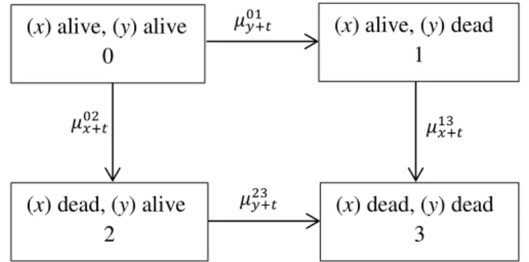
A common example is given by the independent joint life and last survivor models for two lives, (x) and (y). As in practice the two lives are partners, the lives appear in the literature as husband (x) and wife (y). Figure 2 presents the model with state space

𝕁 = {0,1,2,3}.

FIGURE 2 – The independent joint life and last survivor models.

Under the joint life status, TDE for an assured benefit of amount 1 payable immediately upon the first death of (x) and (y) are

𝑑 𝑑𝑡 𝑡𝑉

(0) _{= 𝛿 𝑉}

𝑡 (0)− (𝜇𝑦+𝑡01 + 𝜇𝑥+𝑡02 ) (1 − 𝑉𝑡 (0)) (3.33)

(x) alive, (y) alive 0

𝜇𝑦+𝑡01

𝜇𝑥+𝑡02 𝜇_𝑥+𝑡13

(x) dead, (y) alive 2

(x) alive, (y) dead 1

(x) dead, (y) dead 3

(32)

32

(1)₌ 𝑑 𝑑𝑡 𝑡𝑉

(2)₌ 𝑑 𝑑𝑡 𝑡𝑉

(3)_{= 0.}_(3.34)

Under the last survivor status, TDE for an assured annuity payable continuously at rate of amount 1 per year, while at least one of (x) and (y) is still alive are

(0)_{= 𝛿 𝑉}

𝑡 (0)− 1 − 𝜇𝑦+𝑡01 ( 𝑉𝑡 (1)− 𝑉𝑡 (0)) − 𝜇𝑥+𝑡02 ( 𝑉𝑡 (2)− 𝑉𝑡 (0)) (3.35) 𝑑

𝑑𝑡 𝑡𝑉(1)= 𝛿 𝑉𝑡 (1)− 1 + 𝜇𝑥+𝑡13 𝑉𝑡 (1) (3.36) 𝑑

𝑑𝑡 𝑡𝑉(2)= 𝛿 𝑉𝑡 (2)− 1 + 𝜇𝑦+𝑡23 𝑉𝑡 (2) (3.37) 𝑑

𝑑𝑡 𝑡𝑉

(3)_{= 0.}_(3.38)

(33)

33

4. D

evelopments on Thiele’s differential

equation

4.1 Thiele’s differential equation including payment processes

TDE (3.27) was obtained with deterministic payments. Generalizations of the equation to models with general counting processes driven payments were obtained by Norberg (Norberg 1992a) and Møller (Møller 1993).

The framework is the multiple state model (see 2.4.1) but instead of non-random benefits, a stream of payments generated by a right continuous stochastic process is considered. The payment function is denoted 𝐵_𝑡 and represents the contractual benefits less premiums that are due immediately upon transition. The discount function is

𝑤𝑡 = 𝑒𝑥𝑝( − ∫ 𝛿₀𝑡 𝑠𝑑𝑠). Both functions are defined on some probability space ( Ω, ℱ, 𝑃).

They are adapted to a right-continuous filtration 𝑭 = {ℱ_𝑡}_𝑡≥0 where each ℱ_𝑡 contains all the information available up to time t. Two processes of the history of the policy have to be defined: a multivariate indicator process, denoted 𝐼_𝑡𝑖 , that is equal to 1 or 0 according as the policy is in state i (or not) at time t, and a multivariate counting process for the number of transitions from state i to any state 𝑗, 𝑗 ≠ 𝑖, during the time interval (0, 𝑡],denoted 𝑁_𝑡𝑖𝑗.For any small time interval [𝑡, 𝑡 + 𝑑𝑡], 0 < 𝑡 < ∞ the payment function generated by the life insurance policy is the stochastic differential equation

𝑑𝐵𝑡 = ∑ 𝐼𝑖 𝑡𝑖 𝑑𝐵𝑡𝑖+ ∑ 𝑏𝑖≠𝑗 𝑡𝑖𝑗𝑑𝑁𝑡𝑖𝑗. (4.1)

The future loss random variable at time 𝑡 as defined in 2.3.3, is now for the payment function (4.1)

𝐿𝑡 =_𝑤1_𝑡∫ 𝑤_𝑡∞ 𝜏𝑑𝐵𝜏. (4.2)

The Policy Value is the expected value of (4.2) given the information available up to time t

𝑉

(34)

34

Considering the Policy Value (4.3), the loss of an insurance policy in a given year can be defined as

𝐿 (𝑠, 𝑡] = ∫ 𝑤_𝑠𝑡 𝜏 𝑑𝐵𝜏 + 𝑤𝑡 𝑡𝑉𝑭− 𝑤𝑠 𝑠𝑉𝑭, (4.4)

where the integral accounts for the net outgoing of the period and the other terms give the difference between the reserve that has to be provided at the end of the year and the reserve released at the beginning of the year.

TDE can by derived for payment function (4.1) from Hattendorff’s theorem and using loss definition (4.4) (Norberg 1992a). Hattendorff’s theorem (Sundt and Teugels 2004) states that on a life insurance policy losses in different years have zero means and are uncorrelated, and that the variance is the sum of the variances of the per year losses. From the generalization of Hattendorff’s theorem we come to the fact that (4.4) can be

redefined as the increment over (𝑠, 𝑡] of a martingale generated by the value

𝐿0 = ∫ 𝑤₀𝑡 𝜏𝑑𝐵𝜏. Assuming that 𝐸[𝐿𝑡] < ∞ for each 𝑡 ≥ 0, a martingale denoted 𝑀𝑡 is

defined

𝑀𝑡= 𝐸(𝐿𝑡| ℱ𝑡) = ∫ 𝑤₀𝑡 𝜏𝑑𝐵𝜏+ 𝑤𝑡 𝑡𝑉𝑭. (4.5)

Including (4.1) in (4.5) we come to

𝑀𝑡= 𝐵00+ ∫ 𝑤₀𝑡 𝜏 (∑ 𝐼𝑖 𝜏𝑖 𝑑𝐵𝜏𝑖+ ∑ 𝑏𝑖≠𝑗 𝜏𝑖𝑗𝑑𝑁𝜏𝑖𝑗) + ∑ 𝐼𝑖 𝑡𝑖𝑤𝑡 𝑡𝑉𝑖. (4.6)

Assuming that {𝑀_𝑡}_𝑡≥0is square integrable, then a general representation theorem (Bremaud, 1981) says that 𝑀_𝑡is of the form

𝑀𝑡 = 𝑀0+ ∫ ∑ 𝐻₀𝑡 𝑖≠𝑗 𝜏𝑖𝑗(𝑑𝑁𝜏𝑖𝑗 − 𝐼𝜏𝑖𝜇𝜏𝑖𝑗𝑑𝜏), (4.7)

where the 𝐻𝑖𝑗 are some predictable processes satisfying

𝐸 [∑ ∫ (𝐻𝑖≠𝑗 ₀𝑡 𝜏𝑖𝑗)2𝐼𝜏𝑖𝜇𝜏𝑖𝑗𝑑𝜏] < ∞ (4.8)

and the variance process denoted 〈𝑀_𝑡〉 is given by

𝑑 〈𝑀𝑡〉 (𝑡) = ∑ (𝐻𝑖≠𝑗 𝑡𝑖𝑗)2𝐼𝑡𝑖𝜇𝑡𝑖𝑗𝑑𝑡. (4.9)

(35)

35

𝑏̃_𝑡𝑖𝑗 = 𝑤𝑡 𝑏𝑡𝑖𝑗 (4.10)

𝐵̃𝑡𝑖 = ∫ 𝑤₀𝑡 𝜏𝑑𝐵𝜏𝑖 (4.11)

𝑉̃

𝑡 𝑖 = 𝑤𝑡 𝑡𝑉𝑖 (4.12)

Inserting (4.10), (4.11) and (4.12) in equation (4.6) and using integration by parts to reshape the last term, then

𝑀𝑡 = 𝐵00+ 𝑉̃0 0 + ∫ ∑ 𝐼₀𝑡 𝑖 𝜏𝑖 𝑑(𝐵̃𝑡𝑖+ 𝑉̃𝑡 𝑖) + ∫ ∑ (𝑏̃₀𝑡 𝑖≠𝑗 𝑡𝑖𝑗+ 𝜏𝑉̃𝑗 − 𝑉̃𝜏 𝑖 )𝑑𝑁𝜏𝑖𝑗. (4.13)

Upon identifying the discontinuous parts in (4.7) and (4.13) and afterwards the continuous parts of the same equations, the following theorems were obtained (Norberg 1992a):

Theorem 1: For any continuous discount function and any predictable contractual

functions such that 𝐸 [(∫ 𝑤𝑑𝐵)2] < ∞, the variance process (4.9) is given by

𝐻_𝑡𝑖𝑗 = 𝑏̃_𝑡𝑖𝑗 + 𝑉̃𝜏 𝑗 − 𝑉̃𝜏 𝑖 . (4.14)

The function 𝐻𝑖𝑗in (4.14) can be expressed as

𝐻_𝑡𝑖𝑗 = 𝑤𝑡 𝑅𝑡𝑖𝑗, (4.15)

where 𝑅_𝑡𝑖𝑗 = 𝑏_𝑡𝑖𝑗 + 𝑉_𝑡 𝑗 − 𝑉_𝑡 𝑖 is the amount at risk.

Theorem 2: For any continuous discount function and any predictable contractual

functions such that [𝐸(∫ 𝑤𝑑𝐵)2 < ∞], the following identity holds almost surely

𝐼𝑡𝑖𝑑(𝐵̃𝑡𝑖 + 𝑉̃𝑡 𝑖) + ∑ 𝑗≠𝑖𝐻𝑡𝑖𝑗𝐼𝑡𝑖𝜇𝑡𝑖𝑗𝑑𝑡 = 0. (4.16)

The importance of this result is that (4.16) is a generalization of TDE valid for any counting process and for any predictable benefit function including a lump sum benefit upon survival.

For instance, from (4.16) we can obtain TDE (3.29). Inserting (4.11), (4.12) and (4.15) in (4.16) and using integration by parts for 𝑑 𝑉̃_𝑡 𝑖 = 𝑑𝑤_𝑡 _𝑡𝑉𝑖 + 𝑤_𝑡𝑑 𝑉_𝑡 𝑖 =

(36)

36

𝐼𝑡𝑖𝑑 (∫ 𝑤₀𝑡 𝜏 𝑑𝐵𝜏𝑖) + 𝐼𝑡𝑖(−𝑤𝑡𝛿𝑡 𝑡𝑉𝑖 + 𝑤𝑡𝑑 𝑉𝑡 𝑖) + ∑ 𝑤𝑗≠𝑖 𝑡 𝑅𝑖𝑗𝑡 𝐼𝑡𝑖𝜇𝑡𝑖𝑗𝑑𝑡 = 0. (4.17)

Dividing by 𝑤_𝑡, rearranging and then dividing again by dt, then (3.29) follows

𝑑

𝑑𝑡 𝑡𝑉𝑖 = −𝐵𝑡𝑖+ 𝑉𝑡 𝑖𝛿𝑡− ∑ 𝑅𝑡 𝑖𝑗_𝜇

𝑡 𝑖𝑗 𝑗,𝑗≠𝑖 .

The result is the same TDE obtained for deterministic payments as in 3.7.

4.2 Thiele’s differential equation including stochastic interest rates

The development of life insurance industry creates the need to adapt actuarial models to the development of financial theory. In that sense, versions of TDE can also be obtained with interest governed by stochastic processes of diffusion type, replacing the deterministic interest by a stochastic process (Norberg and Møller 1996). Introducing stochastic interest rate models on Thiele’s equation opens the possibility to manage risk of long term yields on assets corresponding to the reserve.

Following the authors work, the simplest one factor diffusion model will be first studied, and then we shall include two other well-known interest models.

The model considered is the Markov chain model with a stream of payments generated by the stochastic differential equation (4.1). The deterministic discount function 𝑤_(𝑡,𝑢) = 𝑒𝑥𝑝( − ∫ 𝛿_𝑡𝑢 _𝑠𝑑𝑠), 𝑡 < 𝑢is replaced by a stochastic one, by letting the log of discount function be a continuous stochastic process adapted to some filtration 𝑮 = {𝒢_𝑡}_𝑡≥0, representing the economic environment. The source of randomness is modelled using a Brownian motion (Mörters and Peres 2010), 𝑊_𝑡. The stochastic differential equation is

𝑑𝑟𝑡 = 𝛿𝑡𝑑𝑡 + 𝜎𝑡 𝑑𝑊𝑡, (4.18)

(37)

37

𝑟𝑢− 𝑟𝑡 ~ 𝑁(∫ 𝛿_𝑡𝑢 𝑠𝑑𝑠 , ∫ 𝜎_𝑡𝑢 𝑠2𝑑𝑠 ). (4.19)

The discount function is then

𝑤(𝑡,𝑢)′ = 𝐸(𝑤(𝑡,𝑢)| 𝒢𝑡) = 𝐸(𝑒−(𝑟𝑢−𝑟𝑡)| 𝒢𝑡). (4.20)

We can observe that the expectation is of the form 𝐸[𝑒𝜆𝑋], where 𝜆 is a constant and 𝑋~𝑁(∫ 𝛿_𝑡𝑢 _𝑠𝑑𝑠 , ∫ 𝜎_𝑡𝑢 _𝑠2𝑑𝑠 ). Using the moment generating function of a normal

variable, 𝑀(𝜆) = 𝑒𝑥𝑝(𝜇 𝜆 +1

2𝜎2𝜆2) with 𝜇 = ∫ 𝛿𝑠𝑑𝑠 𝑢

𝑡 and 𝜎2 = ∫ 𝜎𝑠2𝑑𝑠 𝑢

𝑡 we arrive to

the discount function for the stochastic interest process (4.18),

𝑤_(𝑡,𝑢)′ = 𝑒𝑥𝑝( − ∫ 𝛿_𝑡𝑢 _𝑠∗𝑑𝑠) (4.21)

with 𝛿_𝑡∗ = 𝛿_𝑡− 1

2 𝜎𝑡2. (4.22)

A version of TDE is obtained by including the force of interest (4.22) in (3.29). The present model is equivalent to the one with deterministic interest.

Another version of TDE can be obtained considering the Vasicek model (Vasicek 1977) and the CIR model (Cox et al.1985). These are time homogeneous models, i.e., their future dynamics do not depend on what the present time 𝑡 is on the calendar. The general stochastic differential equation for both models is

𝑑𝛿𝑡 = 𝑘 (𝑡, 𝛿𝑡)𝑑𝑡 + 𝜎(𝑡, 𝛿𝑡) 𝑑𝑊𝑡. (4.23)

The Vasicek model is an Ornstein-Uhlenberg process (Oksendal 1992), and its dynamics is given by 𝑑𝛿_𝑡 = 𝑘(𝛿̅ − 𝛿_𝑡)𝑑𝑡 + 𝜎𝑑𝑊_𝑡 where 𝑘, 𝛿̅and 𝜎 are positive constants, 𝛿̅ being the long term average force of interest. The CIR model has the same form of drift parameter but includes a different volatility parameter which ensures that

interest remains positive. Its stochastic differential equation is given by

𝑑𝛿𝑡 = 𝑘(𝛿̅ − 𝛿𝑡)𝑑𝑡 + 𝜎√𝛿𝑡𝑑𝑊𝑡.

(38)

38

turn the Policy Value into a stochastic differential equation as it was done in (3.9), the Itô’s formula (Oksendal 1992) has to be applied (Itô’s formula is in appendix B),

𝑑𝑉𝑖_{(𝑡, 𝛿}

𝑡) =_𝑑𝑡𝑑 𝑉𝑖(𝑡, 𝛿𝑡)𝑑𝑡 +_𝑑𝛿𝑑 𝑉𝑖(𝑡, 𝛿𝑡)𝑑𝛿𝑡+ 𝑑

2

𝑑𝛿2𝑉𝑖(𝑡, 𝛿𝑡)

1

2 𝜎2(𝑡, 𝛿𝑡)𝑑𝑡 (4.24)

including (4.23),

𝑑𝑉𝑖(𝑡, 𝛿_𝑡) = 𝑑

𝑑𝑡𝑉𝑖(𝑡, 𝛿𝑡)𝑑𝑡 + 𝑑

𝑑𝛿𝑉𝑖(𝑡, 𝛿𝑡)[𝑘 (𝑡, 𝛿𝑡)𝑑𝑡 + 𝜎(𝑡, 𝛿𝑡)𝑑𝑊𝑡]

+_𝑑𝛿𝑑2₂𝑉𝑖_{(𝑡, 𝛿}

𝑡)1₂ 𝜎2(𝑡, 𝛿𝑡)𝑑𝑡 . (4.25)

Rearranging (4.25) and knowing that 𝑑𝑊_𝑡𝑑𝑡 = 0, then

𝑑

𝑑𝑡𝑉𝑖(𝑡, 𝛿𝑡) = 𝑑

𝑑𝑡𝑉𝑖(𝑡, 𝛿𝑡) + 𝑑

𝑑𝛿𝑉𝑖(𝑡, 𝛿𝑡) 𝑘 (𝑡, 𝛿𝑡) + 𝑑2

1

2 𝜎2(𝑡, 𝛿𝑡). (4.26)

From (4.26) we observe that the difference from the classical TDE (3.27) arises from the last two additional terms. Inserting (3.27) in (4.26), we get

𝑑

𝑑𝑡𝑉𝑖(𝑡, 𝛿𝑡) = 𝛿 𝑉𝑖(𝑡, 𝛿𝑡) − 𝐵𝑡𝑖− ∑ 𝜇𝑡 𝑖𝑗_(𝑏

𝑡𝑖𝑗

𝑗,𝑗≠𝑖 + 𝑉𝑗(𝑡, 𝛿𝑡) − 𝑉𝑖(𝑡, 𝛿𝑡))

+_𝑑𝛿𝑑 𝑉𝑖_{(𝑡, 𝛿}

𝑡) 𝑘 (𝑡, 𝛿𝑡) + 𝑑

2

1

2 𝜎2(𝑡, 𝛿𝑡). (4.27)

TDE (4.27) opens the possibility to study the decomposition of the rate of change of reserves per policyholder for any state i where the model includes a stochastic interest rate process.

4.3 Thiele’s differential equation: a tool for life insurance product development

One of the applications of TDE is the development of new products using the equation as a tool (Ramlau-Hansen 1990 and Norberg 1992b). Some illustrations follow.

(39)

39

𝑏𝑡02= 𝑏𝑡12= 𝑆1+ 𝑉𝑡 𝑥(0) and 𝐵𝑡1 = 𝑏𝑡01 = 0, requiring that 𝑉𝑛 (0) = 𝑉𝑛 (1)= 𝑆2 and 𝑉𝑜 (0)= 0 , equations (3.30) and (3.31) become, respectively,

(0)_{= 𝛿 𝑉}

𝑡 𝑥(0)+ 𝑃 − 𝜇𝑥+𝑡02 𝑆1− 𝜇01𝑥+𝑡 ( 𝑉𝑡 𝑥(1)− 𝑉𝑡 𝑥(0)) (4.28)

and 𝑑

(1)_{= 𝛿 𝑉}

𝑡 𝑥(1)− 𝜇𝑥+𝑡12 𝑆1− 𝜇𝑥+𝑡12 ( 𝑉𝑡 𝑥(0)− 𝑉𝑡 𝑥(1)). (4.29)

Subtracting (4.28) from (4.29) we get,

(1)₋ 𝑑 𝑑𝑡 𝑡 𝑥𝑉

(0) _{= (𝛿 + 𝜇} 𝑥+𝑡 01 _{+ 𝜇}

𝑥+𝑡 12 _{)( 𝑉}

𝑡 𝑥(1)− 𝑉𝑡 𝑥(0)) − 𝑃 + 𝑆1(𝜇𝑥+𝑡02 − 𝜇𝑥+𝑡12 ).

(4.30) The solution of (4.30) in order to the amount at risk as defined in (3.28) is

𝑉𝑡 𝑥(1)− 𝑉𝑡 𝑥(0) = 𝑃 ∫ exp (− ∫ 𝛿 +_𝑡𝑛 _𝑡𝑠 𝜇𝑥+𝑢01 + 𝜇𝑥+𝑢12 𝑑𝑢)𝑑𝑠

+𝑆1∫ exp (− ∫ 𝛿 +_𝑡𝑛 _𝑡𝑠 𝜇𝑥+𝑢01 + 𝜇𝑥+𝑢12 𝑑𝑢)[𝜇𝑥+𝑡12 − 𝜇𝑥+𝑡02 ]𝑑𝑠 . (4.31)

Inserting (4.30) into (4.28) and solving for the rate of premium P the result is the rate of premium of the contract when death benefits depend on the Policy Value. Death benefits may also be set as a fraction 𝛼 > 0 of the Policy Value in the following way:

𝑏𝑡02= 𝑏𝑡12= 𝛼 𝑡𝑉𝑥. Using the same technique, the premium is obtained for this type of

contract (Ramlau-Hansen 1990).

Another approach to develop new insurance products is to set a fluctuation loading to premiums, depending on higher order conditional moments of the present value of payments. Higher order moments of present value are obtained using martingale techniques to avoid multiple integrals (Norberg 1992b).

Considering a life insurance contract with a stochastic payment function (4.1), the qth conditional moment of the present value of payments, denoted 𝑉_𝑡(𝑞)𝑖, given that the policyholder is in state 𝑍(𝑡) = 𝑖, is

𝑉_𝑡(𝑞)𝑖 = 𝐸 [(_𝑣1

𝑡∫ 𝑣𝜏 𝑑𝐵𝜏

𝑛

𝑡 ) 𝑞

| 𝐼𝑡 𝑖 = 1 ] . (4.32)

(40)

40

𝑑 𝑑𝑡𝑉𝑡

(𝑞)𝑖 _{= (𝑞𝛿}

𝑡𝑖 + 𝜇𝑡𝑖) 𝑉𝑡(𝑞)𝑖− 𝑞𝑏𝑡𝑖 𝑉𝑡(𝑞−1)𝑖− ∑ 𝜇𝑗≠𝑖 𝑖𝑗𝑡 ∑ (𝑞𝑟=0 𝑞𝑟) (𝑏𝑡𝑖𝑗)𝑟𝑉𝑡(𝑞−𝑟)𝑗 (4.33)

valid on (0, n) ∖ 𝔇 and subject to the conditions

𝑉_𝑡−(𝑞)𝑖 = ∑ (𝑞_𝑟=0 𝑞_𝑟) (𝐵𝑡𝑖− 𝐵𝑡−𝑖 )𝑟 𝑉𝑡(𝑞−𝑟)𝑖, 𝑡 ∈ 𝔇 (4.34)

where 𝔇 = {𝑡₀, … , 𝑡_𝑛} is the set of times listed in chronological order, where jumps to other states can occur so that a lump sum 𝑏_𝑡𝑖𝑗 is then payable at time 𝑡.

TDE is the particular case when q=1 and all forces of interest 𝛿𝑖 are equal:

𝑑

𝑑𝑡𝑉𝑡(1)𝑖 = 𝛿𝑡 𝑉𝑡(1)𝑖 − 𝐵𝑡𝑖 − ∑ 𝜇𝑡 𝑖𝑗 _(𝑏

𝑡𝑖𝑗+ 𝑉𝑡(1)𝑗− 𝑉𝑡(1)𝑖)

𝑗≠𝑖 . (3.27)

Central moments, denoted 𝑚_𝑡(𝑞)𝑖, can also be obtained:

𝑚_𝑡(𝑞)𝑖 = ∑ (𝑞_𝑟)(−1)𝑞−𝑝_𝑉 𝑡(𝑝)𝑖( 𝑞

𝑝=0 𝑉𝑡(1)𝑖)𝑞−𝑝. (4.35)

When q=1 the result is 𝑚_𝑡(1)𝑖 = 𝑉_𝑡(1)𝑖.

As an example, premiums can include a loading proportional to the variance, as follows: 𝛼𝑚_𝑡(2)𝑖, 𝛼 > 0.

4.4 Thiele’s differential equation for a closed insurance portfolio

From TDE (3.29) derived for a single policy with non-random benefits, the Policy Value for a closed insurance portfolio can be derived (Linnemann 1993). The results may be used to make actuarial consistent projections of the development of such an insurance portfolio. It also gives the theoretical basis to perform the Thiele control as we shall see.First a reformulation of equation (3.29) is necessary to then come to TDE for the insurance portfolio.