Impacts of beaver dams on hydrologic and temperature regimes in a mountain stream

(1)

HESSD

12, 839–878, 2015

Impacts of beaver dams on hydrologic

and temperature regimes in a mountain stream

M. Majerova et al.

Title Page

Abstract Introduction

Conclusions References

Tables Figures

◭ ◮

Back Close

Full Screen / Esc

Printer-friendly Version

Interactive Discussion

Discussion

P

a

per

|

Discussion

P

a

per

|

Discussion

P

a

per

|

Discussion

P

a

per

|

Hydrol. Earth Syst. Sci. Discuss., 12, 839–878, 2015 www.hydrol-earth-syst-sci-discuss.net/12/839/2015/ doi:10.5194/hessd-12-839-2015

This discussion paper is/has been under review for the journal Hydrology and Earth System Sciences (HESS). Please refer to the corresponding final paper in HESS if available.

Impacts of beaver dams on hydrologic

and temperature regimes in a mountain

stream

M. Majerova1, B. T. Neilson1, N. M. Schmadel1, J. M. Wheaton2, and C. J. Snow1

1

Utah Water Research Laboratory, Department of Civil and Environmental Engineering, Utah State University, 8200 Old Main Hill, Logan, Utah, 84322-8200, USA

2

Department of Watershed Sciences, Utah State University, 8200 Old Main Hill, Logan, Utah, 84322-8200, USA

Received: 3 December 2014 – Accepted: 28 December 2014 – Published: 22 January 2015

Correspondence to: M. Majerova ([email protected]) and B. T. Neilson ([email protected])

(2)

HESSD

12, 839–878, 2015

M. Majerova et al.

Title Page

Tables Figures

◭ ◮

Back Close

Full Screen / Esc

Discussion

P

a

per

|

Discussion

P

a

per

|

Discussion

P

a

per

|

Discussion

P

a

per

|

Abstract

Beaver dams affect hydrologic processes, channel complexity, and stream tempera-ture by increasing inundated areas and influencing groundwater-surface water interac-tions. We explored the impacts of beaver dams on hydrologic and temperature regimes at different spatial and temporal scales within a mountain stream in northern Utah

5

over a three-year period spanning pre- and post-beaver colonization. Using continuous stream discharge, stream temperature, synoptic tracer experiments, and groundwater elevation measurements we documented pre-beaver conditions in the first year of the study. In the second year, we captured the initial effects of three beaver dams, while the third year included the effects of ten dams. After beaver colonization, reach scale

10

discharge observations showed a shift from slightly losing to gaining. However, at the smaller sub-reach scale, the discharge gains and losses increased in variability due to more complex flow pathways with beaver dams forcing overland flow and increas-ing surface and subsurface storage. At the reach scale, temperatures were found to increase by 0.38◦C (3.8 %), which in part is explained by a 230 % increase in mean

15

reach residence time. At the smallest, beaver dam scale, there were notable increases in the thermal heterogeneity where warmer and cooler niches were created. Through the quantification of hydrologic and thermal changes at different spatial and temporal scales, we document increased variability during post-beaver colonization and high-light the need to understand the impacts of beaver dams on stream ecosystems and

20

their potential role in stream restoration.

1 Introduction

Beaver dams create ponds that change surface water elevations, alter channel mor-phology, and decrease flow velocities (Gurnell, 1998; Meentemeyer and Butler, 1999; Pollock et al., 2007; Rosell et al., 2005). These ponds and the overflow side channels

25

(3)

HESSD

12, 839–878, 2015

M. Majerova et al.

Title Page

Tables Figures

◭ ◮

Back Close

Full Screen / Esc

Discussion

P

a

per

|

Discussion

P

a

per

|

Discussion

P

a

per

|

Discussion

P

a

per

|

residence time, and depositional areas for sediments. The increased storage attenu-ates hydrographs (Gurnell, 1998) and can increase base flow (Nyssen et al., 2011). Specifically in the beaver ponds, water infiltration through the bed and adjacent banks influences local groundwater elevations (Hill and Duval, 2009). Within the stream chan-nel, beaver dams alter hydraulic gradients (Lautz and Siegel, 2006) that increase the

5

potential for hyporheic exchange (Lautz and Siegel, 2006). Such changes in channel morphology and hydrology alter stream temperature regimes. Warming due to solar radiation can be a key factor due to increased water surface area (Cook, 1940). Fur-ther, foraging and extensive inundation can lead to loss of riparian vegetation that de-creases riparian canopy and the associated shading influences (Beschta et al., 1987).

10

Changes in groundwater–surface water interactions can also impact the overall temper-ature regime (e.g., upwelling zones decrease tempertemper-atures below beaver dams (Fanelli and Lautz, 2008; White, 1990). Regardless of this implied connection between hydro-logic and stream temperature changes due to beaver dam construction, most studies have investigated these changes separately. Furthermore, the temporal and spatial

15

scales considered within individual studies vary widely, leading to inconsistent conclu-sions regarding beaver dam impacts on stream systems (Kemp et al., 2012).

When considering hydrologic influences at the beaver dam scale (which includes the beaver dam structure, the upstream ponded area, and the section below the dam), Briggs et al. (2012) found a connection between streambed morphologies formed

up-20

stream of beaver pond and hyporheic flow patterns. Similarly, Lautz and Siegel (2006) showed that beaver dams promoted higher infiltration of surface water into the subsur-face. Janzen and Westbrook (2011) found enhanced vertical recharge between stream and underlying aquifer upstream of the dams. They also found that the hyporheic flow-paths surrounding beaver dams were longer than expected. Nyssen et al. (2011)

stud-25

(4)

HESSD

12, 839–878, 2015

M. Majerova et al.

Title Page

Tables Figures

◭ ◮

Back Close

Full Screen / Esc

Discussion

P

a

per

|

Discussion

P

a

per

|

Discussion

P

a

per

|

Discussion

P

a

per

|

floods increased over 20 years and peak flows were decreased and delayed by ap-proximately a day. In contrast, some argue that while beaver dams affect downstream delivery, they provide minimal retention during large runoffevents (Burns and McDon-nell, 1998).

The documented impacts of beaver dams on temperature are more variable. Some

5

studies found that beaver dams and beaver ponds cause overall increases in down-stream temperatures (Andersen, 2011; Margolis et al., 2001; Salyer, 1935; McRae and Edwards, 1994; Shetter and Whalls, 1955) with reported values as high as 9◦C during summer months (Margolis et al., 2001). Fuller and Peckarsky (2011) also observed increases in temperatures below low-head beaver dams, but a cooling effect below

10

high-head beaver dams. At the longer reach scale (22 km), Talabere (2002) found no significant influence of beaver dams on stream temperature. A recent literature review regarding the impacts of beaver dams on fish further summarizes such inconsistent findings. Kemp et al. (2012) cited 13 articles that argued beaver dams provided thermal refugia and 11 articles that argued negative impacts from altered thermal regime (i.e.,

15

detrimental increases in summer temperatures). Interestingly, this review also pointed out that of the 13 articles claiming temperature benefits of beaver dams, only seven were data driven and the remaining six were speculative. By contrast, of the 11 arti-cles showing temperature impairments, only one was data driven while the rest were speculative. Another recent literature review regarding the e_ffects of beaver activity in

20

stream restoration and management further revealed that a majority of studies cover small spatial scale areas (e.g., small reach scales), are mainly qualitative, and many hypotheses are supported only by anecdotal or speculative information (Gibson and Olden, 2014). Particularly in the context of stream management, where beaver have recently been considered as a potential restoration tool (e.g., Utah Beaver

Manage-25

ment Plan), a more quantitative understanding of the hydrologic and thermal impacts of beaver within stream systems is critical.

(5)

HESSD

12, 839–878, 2015

M. Majerova et al.

Title Page

Tables Figures

◭ ◮

Back Close

Full Screen / Esc

Discussion

P

a

per

|

Discussion

P

a

per

|

Discussion

P

a

per

|

Discussion

P

a

per

|

data driven studies across multiple spatial and temporal scales. In an effort to link hy-drologic and temperature responses due to beaver dam development, we present data from different spatial (reach, sub-reach, and beaver dam) and temporal scales (instan-taneous to continuous three-year time series) that span a period prior to and during the establishment of 10 beaver dams. We illustrate how the development of beaver dams

5

shifts instream hydrologic and thermal responses. More specifically, a losing reach (pre-beaver) was transformed to a gaining reach (post-beaver) while simultaneously increasing stream temperatures.

Site description

Curtis Creek, a tributary of the Blacksmith Fork River of Northern Utah drains a portion

10

of the Bear River Range. Curtis Creek is a first-order perennial mountain stream with intermittent tributaries. The mountainous watershed includes a combination of hard sedimentary rock, Paleozoic and Precambrian limestone bedrock that is strongly in-durated. The valley broadens in the lower portion of Curtis Creek and is primarily dom-inated by remnant low-angle alluvial fans. The valley bottom is comprised of a mix of

15

longitudinally stepped floodplain surfaces and channel that are both partly confined by coarse-grained alluvial fan deposits with gravel, cobble, boulders and some soil devel-opment. These stepped floodplains are infrequently inundated by the modest spring-snowmelt flow regime, and reflect surfaces created by relic beaver ponds and beaver dam flooding.

20

Data were gathered in a 750 m long study site on the lower portion of Curtis Creek that is located about 15 mi east of Hyrum, Utah at Hardware Ranch (an elk refuge op-erated by the Utah Division of Wildlife Resources – UDWR). The study reach has a rel-ative steep streambed slope of 0.035, supporting a bed of coarse gravel to large cobble with some man-made boulder vortex weirs placed within the new channel with a

mean-25

(6)

leav-HESSD

12, 839–878, 2015

M. Majerova et al.

Title Page

Tables Figures

◭ ◮

Back Close

Full Screen / Esc

Discussion

P

a

per

|

Discussion

P

a

per

|

Discussion

P

a

per

|

Discussion

P

a

per

|

ing portions of the original channel abandoned. The banks of the realigned channel were stabilized with boulders, root wads, logs, and erosion control blankets.

The riparian area surrounding the channel prior to and following relocation was heav-ily grazed by elk and did not support woody riparian vegetation. Roughly around 2005, grazing pressure was lessened and the area was fenced (though some grazing was still

5

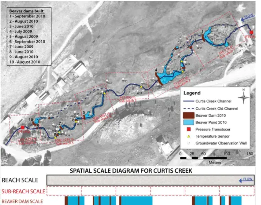
allowed). This facilitated some modest recovery of the riparian woody vegetation which was enough to attract beaver. In early summer of 2009, beaver colonization began with beaver dam 7 constructed in the middle of the study reach (Fig. 1). Beaver dams 4 and 5 were also completed during summer 2009. New beaver dams (3 and 8) were established early-summer 2010 and by the late summer-early fall, dams 2, 6, 9, and 10

10

were completed. By the end of fall 2010, beaver dam 1 was built at the upstream end of the study reach resulting in a total of 10 beaver dams with an average height of 1 m. In addition, two small (less than 0.5 m in height) beaver dams were constructed in the old channel (Fig. 1, dams without numbers). Beaver built seven of their dams using the artificial restoration structures as foundations. By the end of fall 2010, the channel

con-15

sisted of sections with flowing water (main channel and side channels), ponded water (beaver ponds), and beaver dam structures (Figs. 1 and 7). The resulting dam density by 2010 was 13.3 dams km−1.

2 Methods

The field site was originally instrumented with pressure transducers, temperature

sen-20

sors, and groundwater observation wells to investigate groundwater–surface water in-teractions in the absence of beaver. After one year of data collection, beaver coloniza-tion occurred within the study reach, changing the objectives of the study. In short, it produced the perfect accidental experiment and a unique opportunity to quantify fundamental hydrologic and thermal impacts of beaver dam construction on stream

25

(7)

HESSD

12, 839–878, 2015

M. Majerova et al.

Title Page

Tables Figures

◭ ◮

Back Close

Full Screen / Esc

Discussion

P

a

per

|

Discussion

P

a

per

|

Discussion

P

a

per

|

Discussion

P

a

per

|

(Table 1, Fig. 1). Flow information was collected at the reach and sub-reach scale to compare influences of individual beaver dams and cumulative impacts. In addition, groundwater levels were observed within the floodplain of the study reach. To explore the corresponding impacts of dams on thermal regimes, stream temperature data were collected and analyzed at the reach, sub-reach and beaver dam scales. Both the

hy-5

drologic and temperature data collection took place over different temporal scales and the frequency varied from instantaneous measurements to continuous data throughout the three-year period.

2.1 Data collection

The study reach boundaries were set following a previous study (Schmadel et al., 2010)

10

and locations along the reach were denoted by distance downstream from an arbitrary datum set upstream of the study reach (Fig. 1). Water level and temperature were measured using KWK Technologies® SPXD™ 610 (0–5 psig) (Spokane, Washington) pressure transducers (PT) with vented cables and Campbell Scientific® CR-206 data loggers (Logan, Utah) at the upstream (PT515, Fig. 1) and downstream study reach

15

limit (PT1252, Fig. 1). Water level and temperature were measured at 30 s intervals and five-minute averages were recorded. Discharges were measured at each PT un-der the full range of flow conditions using the velocity-area method to establish rating curves. The flow velocity was recorded with a Marsh McBirney Inc.®Flo-Mate™(Model 200, Frederick, Maryland). To provide a local comparison of hydrologic responses due

20

to beaver activity, continuous discharge data were similarly collected at the bounds of a control reach approximately 535 m long without any beaver activity located immedi-ately upstream from our study reach (PT0).

The study reach was further divided into six sub-reaches, ranging from 56 to 168 m and numbered sequentially downstream (Fig. 1). The six sub-reaches spanned

indi-25

(8)

(sub-HESSD

12, 839–878, 2015

M. Majerova et al.

Title Page

Tables Figures

◭ ◮

Back Close

Full Screen / Esc

Discussion

P

a

per

|

Discussion

P

a

per

|

Discussion

P

a

per

|

Discussion

P

a

per

|

reach 3). Dilution gaging was conducted at the sub-reach scale on 16 July 2008 (pre-beaver) and 19 July 2010 (post-(pre-beaver) to provide a longitudinal understanding of flow variability. As described within Schmadel et al. (2010, 2014), chloride (from NaCl) was used as a conservative tracer (Zellweger, 1994) and rhodamine WT was used as a vi-sual indicator for a qualitative assessment of mixing. Tracer responses were measured

5

following an instantaneous tracer injection starting at the downstream end of the study reach and then moving upstream to individual sub-reach limits. Each response was measured with specific conductance (SC) (electrical conductivity normalized to 25◦C as a surrogate to chloride concentrations) at one-second intervals using YSI® son-des (models 600 LS and 600 XLM, Yellow Springs, Ohio) calibrated in the field. The

10

background SC was corrected to zero (Gooseffand McGlynn, 2005; Payn et al., 2009) and each corrected response was correlated to chloride concentrations with calibration regressions.

To capture changes in groundwater levels throughout the reach, groundwater ob-servation wells were installed in June 2008 (Fig. 1). These wells were constructed

15

from half inch polyvinyl chloride (PVC), 2 m in length with 40 cm of perforation covered with 2 mm flexible nylon screen to exclude soil. Elevations were established for individ-ual wells using a total station and later using differential rtkGPS (Trimble® R8, Global Navigation Satellite System, Dayton, Ohio). Groundwater levels were determined by measuring distance from the top of each well to the groundwater surface level in each

20

well using a Solinst® electronic well sounder (Model 101 Mini, Georgetown, Ontario, Canada).

At the finer, beaver dam scale, temperature measurements were collected above and below individual beaver dams at 10 min intervals using Onset®HOBO®Temp Pro V2 (Bourne, Massachusetts) deployed from 2 September to 15 October 2010 (Fig. 1,

25

Tables 1 and 2). The temperature sensors were wrapped in aluminum foil to reduce solar radiation influence in slower moving water.

(9)

HESSD

12, 839–878, 2015

M. Majerova et al.

Title Page

Tables Figures

◭ ◮

Back Close

Full Screen / Esc

Discussion

P

a

per

|

Discussion

P

a

per

|

Discussion

P

a

per

|

Discussion

P

a

per

|

captured with high resolution aerial imagery available through the Utah Automated Ge-ographic Reference Center (AGRC). Post colonization, NIR (Near Infrared) and RGB (Red-Green-Blue) aerial imagery were collected using Aggie Air UAVs (Unmanned Aerial Vehicle) in 2010. Aggie Air flights that additionally included thermal aerial im-ages were completed in 2011–2013.

5

2.2 Data analysis

At the reach scale, the five-minute continuous stage and temperature data recorded at the study reach boundaries were averaged to daily values to illustrate changes over the three-year study period. Data from the winter months were excluded from the anal-ysis because they were influenced by ice buildup in the stream. Rating curves were

10

developed from the measured discharges and continuous stage from PTs in the form (Cey et al., 1998; Rantz, 1982):

Q₌aZb (1)

whereQis the predicted discharge (L s−1),aandbare the regression parameters, and Z is the stage measured by the pressure transducer (m). Nonlinear regression was

15

used to estimatea andbas described within Schmadel et al. (2010). The continuous discharge estimates provided continuous estimates of net change in stream discharge (_∆Q) at the reach scale (downstream discharge minus upstream discharge). To illus-trate percent net change (%∆Q),∆Qwas normalized by upstream discharge (Qat the upstream reach boundary). The net change in stream temperature (∆T, downstream

20

(10)

HESSD

12, 839–878, 2015

M. Majerova et al.

Title Page

Tables Figures

◭ ◮

Back Close

Full Screen / Esc

Discussion

P

a

per

|

Discussion

P

a

per

|

Discussion

P

a

per

|

Discussion

P

a

per

|

At the finer, sub-reach scale, stream discharge was calculated at each sub-reach limit from dilution gaging using (Kilpatrick and Cobb, 1985):

Q₌ M

τ

R

0

(C(t)−Cb(t))dt

= _τ M R

0

C(t)dt

(2)

whereQis the stream discharge (L s−1),M is the mass of solute tracer injected (mg), C(t) is the tracer concentration (mg L−1),C_b(t) is the background tracer concentration

5

(corrected to zero) (mg L−1_),_t _{is time (s), and}_τ _{is the measurement time period from} tracer injection to last detection (s). The net ∆Q was also estimated at the limits of each sub-reach (Fig. 1). The net∆Qfor each sub-reach was again normalized by the discharge at the corresponding upstream sub-reach limit resulting in a net %∆Q to allow for direct comparison between sub-reaches. Uncertainty in the estimates was

10

quantified using the same technique presented in Schmadel et al. (2010). Tracer mass recovery through each sub-reach was calculated to provide information regarding flow diversions within and possible returns to some sub-reaches. In addition, mean res-idence times (µ_t) for individual sub-reaches were estimated from the first temporal moment or expected value of each recovered tracer response as:

15

µ_t₌

τ

R

0

tC_D(t)dt

τ

R

0

C_D(t)dt

(3)

where C_D(t) is the recovered tracer response at the downstream sub-reach limit (mg L−1_).

To further understand hydrologic impacts of beaver dam construction, groundwater elevation data grouped by each sub-reach were evaluated for 2008, 2009, and 2011.

(11)

HESSD

12, 839–878, 2015

M. Majerova et al.

Title Page

Tables Figures

◭ ◮

Back Close

Full Screen / Esc

Discussion

P

a

per

|

Discussion

P

a

per

|

Discussion

P

a

per

|

Discussion

P

a

per

|

There were no groundwater elevation data collected in 2010 and thus post-beaver colo-nization period was represented by the 2011 data. Due to the established groundwater observation wells not being distributed evenly throughout the study reach, changes in groundwater over the study period are only available for sub-reaches 2, 3, and 5.

The temperature impacts at the beaver dam scale were quantified from the data

5

above and below individual beaver dams (3, 4, 5, 7, and 8) from fall 2010 (Fig. 1 and Table 2). In case of beaver dam 7 and 8, the ponded water from beaver dam 8 extended to beaver dam 7. Therefore, we used data above dam 7 and below dam 8. A 24 h moving average was calculated from the data to detect temporal trends other than diurnal patterns. The net temperature change, ∆T, for each individual beaver

10

dam was calculated by subtracting the temperature above the beaver dam from the temperature below the beaver dam. A positive change represented net warming, while a negative change represented net cooling below the beaver dams. The area of flowing water (represented by the stream channel) and ponded water from the beaver dams was digitized and calculated from the 2006 (pre-beaver conditions) and 2010

(post-15

beaver colonization conditions) imagery (Table 3). The main channel water volume for pre- and post-beaver dams were also estimated based on one-dimensional HEC-RAS hydraulic model built to replicate the two di_fferent states (Table 3).

3 Results

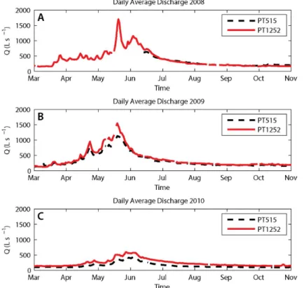
3.1 Reach scale responses 20

At the reach scale, the average daily discharge (Fig. 2) illustrates the seasonal varia-tions and changes in flow condivaria-tions at PT515 (inflow) and PT1252 (outflow) for 2008 through 2010. The 2008 and 2009 flows were fairly comparable with peak flows at PT1252 of 1698 and 1549 L s−1, respectively. The 2010 flows were, however, one third of peak flow in comparison to previous years (592 L s−1 at PT1252). The impacts of

25

(12)

HESSD

12, 839–878, 2015

M. Majerova et al.

Title Page

Tables Figures

◭ ◮

Back Close

Full Screen / Esc

Discussion

P

a

per

|

Discussion

P

a

per

|

Discussion

P

a

per

|

Discussion

P

a

per

|

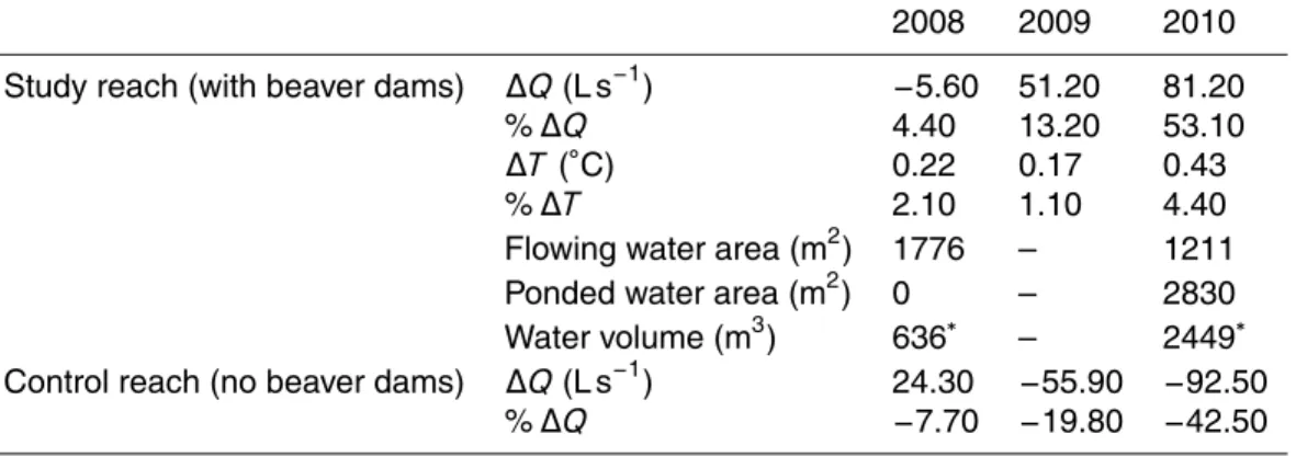
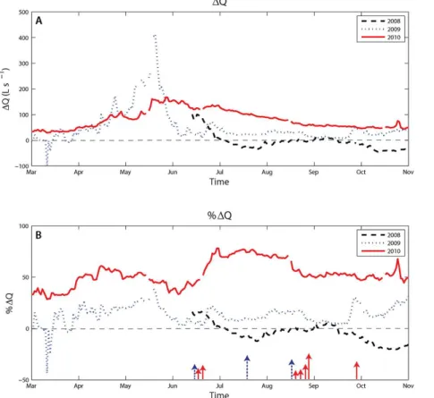
and in the year-to-year variability in net∆Qand %∆Q(Fig. 3). Negative changes indi-cate a net losing reach while positive values indiindi-cate net gains in flow. The daily aver-age value for March–October of 2008 (pre-beaver) was−5.6 L s−1for∆Qand −4.4 % for %∆Q. As the beaver dams were built and increased in number, the average val-ues of∆Qand %∆Qincreased to 51.2 L s−1and 13.2 % in 2009 and to 81.2 L s−1and

5

53.1 % in 2010, respectively.

Across shorter temporal scales, variability within each season of each year was also apparent. Even though data are only available for short portion of the spring period in 2008, the reach was gaining. In July 2008, the %∆Q became negative suggesting that the reach was losing during the spring flood recession. In early spring of 2009, the

10

reach shifted from losing to gaining. However, the reach did not switch back to losing conditions during lower flows and gains were approximately 10 % during the months of June, July, and August. In September 2009, the %∆Q further increased to 30 % over one week and was followed by a slow decrease of approximately 20 % the following two weeks before increasing again. Similar gaining conditions continued throughout

15

2009 and into 2010. In 2010, another increase in %∆Q was observed in April at the beginning of snowmelt and reached up to 60 %. The greatest %_∆Qoccurred at the end of June 2010 reaching approximately 80 % (Fig. 3). This sort of drastic change may be partially affected by irrigation patterns in nearby fields during summer months.

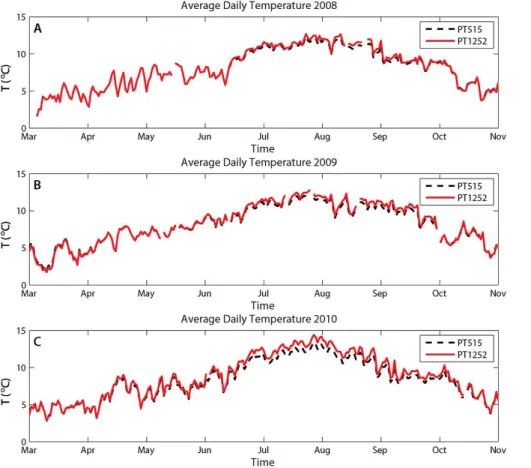
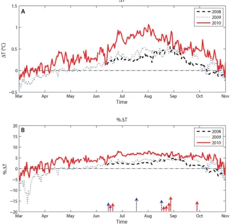
At the reach scale, stream temperatures consistently increased during the summer

20

with peaks occurring at the end of July and beginning of August, and some periods of cooling within the reach in the fall and winter for all three years (Fig. 4). Net and percent changes in temperature (_∆T and %_∆T) show a warming trend from 2008 to 2010 corresponding to the increase in the number of dams (Fig. 5). In 2008, the av-erage daily∆T was 0.22◦C and in 2010 the average∆T was 0.43◦C. The average

in-25

(13)

HESSD

12, 839–878, 2015

M. Majerova et al.

Title Page

Tables Figures

◭ ◮

Back Close

Full Screen / Esc

Discussion

P

a

per

|

Discussion

P

a

per

|

Discussion

P

a

per

|

Discussion

P

a

per

|

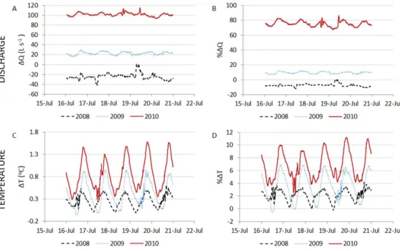
Reach scale data from a smaller temporal scale (a five-day period in July) illustrates the links between discharge and temperature patterns associated with beaver dam construction (Fig. 6). Comparison of ∆Q and %∆Q show similar trends to those in Fig. 3 (i.e., an increase in the amount of water gained over the reach each year), but with diurnal patterns. The %∆Q for 2010 shows approximate 80 % increase in

5

discharge when compared to 2008 (Fig. 6b). The transformation from losing in 2008 to gaining in 2010 is also more pronounced at this shorter five-day scale. Similarly, when comparing∆T and %∆T values there is an average increase of 0.6◦C and 4.6 % from 2008 to 2010, respectively. The data also contain a diurnal pattern with a maximum difference of 1.1◦C (8 %) between 2008 and 2010 (Fig. 6c and d). The∆T values show

10

that the range of temperature di_fferences during the day doubled in 2010. With this transition from a losing to gaining reach, one might expect a decrease in temperature during the summer due to the addition of colder groundwater. However, there was instead increased warming over the study reach. In 2008, the flowing water surface area was estimated to be 1776 m2 with no ponded area. In 2010, the flowing water

15

surface area decreased to 1211 m2 with the ponded area covering about 2830 m2. In the end, the water surface area in 2010 had more than doubled (Fig. 7, Table 3).

3.2 Sub-reach scale responses

With an increase in the number of beaver dams for each consecutive year, the ground-water elevation increased in sub-reaches as shown by the changes in the annual

dis-20

tribution and median values (Fig. 8, Fig. SI2 in the Supplement). The response was greatest for sub-reach 2, where median groundwater levels increased approximately 0.03 m during the first year (2008–2009) and by another 0.34 m from 2009 to 2011. For sub-reaches 3 and 5, median groundwater levels increased by 0.02 and 0.12 m from 2008 to 2009, respectively. From 2009 to 2011, these levels increased further by

25

(14)

HESSD

12, 839–878, 2015

M. Majerova et al.

Title Page

Tables Figures

◭ ◮

Back Close

Full Screen / Esc

Discussion

P

a

per

|

Discussion

P

a

per

|

Discussion

P

a

per

|

Discussion

P

a

per

|

gaining over the study period. However, sub-reach 5 is generally neutral in 2008 and is more commonly losing in surface water in 2009 and 2010 (Fig. 8, Supplement Fig. 2).

Groundwater–surface water exchanges in the study reach prior to beaver dam in-fluences were documented in Schmadel et al. (2014). Discharge estimated at various locations longitudinally illustrates the variability in flows prior to beaver dam influences

5

(Fig. 9a) and the sub-reach scale %∆Qshowed some sub-reaches gaining while oth-ers losing (Fig. 9b). The 2010 discharge values showed greater variability after beaver dams were constructed in the reach (Fig. 9a). In contrast with the yearly average head gradient (Fig. 8), the net %_∆Qin sub-reach 2 shows a transition from gaining in 2008 to losing in 2010, sub-reach 3 from neutral to gaining, and sub-reach 5 from neutral

10

to losing in 2010 (Fig. 9b). Mass recoveries from the dilution gaging show the percent of mass loss and gain changed significantly from 2008 to 2010. In 2008, the mean percent mass losses for individual sub-reaches from 2 to 6 were−3.1,−13.2,−19.7, −20.7, and−9.7 %, respectively. In 2010, the mean percent mass losses were−103.7, −0.3,−9.5,−62.0, and−15.4 % for the same sub-reaches.

15

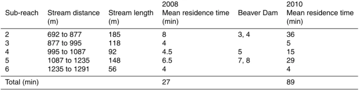
Mean residence times estimated from the 2008 and 2010 tracer studies show an increase for all sub-reaches containing beaver dams (Table 4). The biggest change was observed in sub-reach 2 where beaver dam 4, with the largest pond area, was located (Fig. 1). The second greatest increase occurred in sub-reach 5 where a series of dams and ponds covered approximately 50 % of the sub-reach length. The increase

20

in sub-reach scale residence times translates into an overall reach scale increase of 62 min or 230 %.

3.3 Beaver dam scale responses

The spatial and temporal temperature differences observed between individual beaver dams from a two-day period show that each dam influences the system di_fferently

25

(15)

down-HESSD

12, 839–878, 2015

M. Majerova et al.

Title Page

Tables Figures

◭ ◮

Back Close

Full Screen / Esc

Discussion

P

a

per

|

Discussion

P

a

per

|

Discussion

P

a

per

|

Discussion

P

a

per

|

stream warming trend which cumulatively propagated downstream below beaver dam 8 (Supplement Fig. 3). Although, the temperature increase for each dam was gener-ally within the accuracy of the temperature sensor (±0.2◦C), the cumulative impact of multiple dams showed more significant downstream warming.

Based on the data shown within Fig. 10, daily ranges (daily maximum minus daily

5

minimum values) of temperature differences below and above each beaver dam (∆T) provide additional information regarding the spatial variability among individual dams within each day (Fig. 11a). However, when looking at 24 h moving averages (Fig. 11b), ∆T values fall within the accuracy of the sensors and highlight the importance of the temporal scale (frequency) of measurements when determining the impacts of beaver

10

dams on stream systems.

4 Discussion

While many studies exist regarding the influence of beaver dams on the local hydro-logic and temperature regimes, the majority of these studies lack sufficient quantitative field measurements across appropriate spatial (beaver dam to reach scale) and

tem-15

poral scales (instantaneous to continuous over a period of years) to draw meaningful conclusions (Kemp et al., 2012; Gibson and Olden, 2014). Furthermore, the results are often inappropriately generalized beyond the scales of the observations. Our re-sults quantify the influences of beaver dams on a stream flow and temperatures while demonstrating how beaver dams impact stream hydrologic and temperature regimes

20

at di_fferent spatial and temporal scales.

The reach scale results of our study suggest an overall increase in∆Qfrom 2008 to 2010 based on changes in flow conditions due to beaver dam building activity (Fig. 2). The increases in gains during the spring can be attributed to surface and subsurface lateral inflows. However, the impacts of the beaver dams are more apparent during low

25

(16)

HESSD

12, 839–878, 2015

M. Majerova et al.

Title Page

Tables Figures

◭ ◮

Back Close

Full Screen / Esc

Discussion

P

a

per

|

Discussion

P

a

per

|

Discussion

P

a

per

|

Discussion

P

a

per

|

discharge is more evident. In summer and fall of 2008, the reach is in equilibrium or slightly losing water. In contrast, the reach is gaining water during these same sum-mer and fall months of 2009. This trend continues and is more pronounced as beaver dams continue being built and the cumulative impact of multiple beaver dams results in constant gains in 2010 (Fig. 3b). The dominant hydrologic processes influencing the

5

study reach clearly changed over the period of three years. To provide a comparison, we can use baseline∆Q and %∆Qfrom the control reach just upstream for the same three-year period (Table 3). These data show that the control reach was losing water for all three years except for summer of 2008. In contrast to the beaver impacted study reach, the losing trend in the control reach is more pronounced with each year and it is

10

at its maximum in 2010.

When considering the smaller spatial scales (sub-reach, beaver dam) there is great variability in terms of losses and gains that are not fully understood from the reach scale observations in the study reach with beaver dams (Figs. 8 and 9, Table 4). This variability is due to many different mechanisms occurring in and around beaver dams,

15

including groundwater–surface water exchanges (Lautz and Siegel, 2006; Janzen and Westbrook, 2011). However, the sub-reach scale variability in this study (Fig. 9) was primarily due to high crest dams forcing year round overbank flow. Much of the over-bank flow was either returned to the main channel through side channels or was di-verted to the o_ff-channel beaver ponds. These changes in flowpaths influenced the

20

mass recovery in our tracer study in 2010, when the highest mass loss occurred in sub-reaches with big beaver dams and multiple side channels. The dynamic activity of beaver, through construction and maintenance of dams, and natural seasonal changes in flow lead to a diverse range of hydrologic responses resulting in the spatial and tem-poral variability of gains and losses through the study reach. The dilution gaging results

25

(17)

HESSD

12, 839–878, 2015

M. Majerova et al.

Title Page

Tables Figures

◭ ◮

Back Close

Full Screen / Esc

Discussion

P

a

per

|

Discussion

P

a

per

|

Discussion

P

a

per

|

Discussion

P

a

per

|

and repeated measurements, and also show that the differences in measurement tech-niques can lead to different conclusions as discussed within Schmadel et al. (2014).

Our temperature results demonstrate the considerable spatial and temporal variabil-ity in stream temperature caused by beaver dams. We captured the warming effect at the reach scale over a period of three years (Figs. 4 and 5). However, the data at

5

this scale do not portray the thermal heterogeneity illustrated by the beaver dam scale temperatures (Figs. 10 and 11). Similarly, the temporal scale is of importance when de-termining impacts of beaver dams. For example, the 5 min-interval temperature record captured temperature fluctuations during the day that may play an important role in fish habitat management and restoration (Fig. 6c and d). This daily variability would not be

10

captured if only daily averages or instantaneous measurements were recorded. The lag times in peak temperatures from 2008 to 2010 (more apparent at shorter temporal scales (Supplement Fig. 1) are likely due to different flow conditions, air temperatures, solar radiation, precipitation, and channel morphology.

To understand the significance of simultaneously considering the spatial and

tem-15

poral scale of measurements, Figs. 10 and 11 illustrate the temperature variability for five beaver dams while providing a comparison between the dams. Individual beaver dams introduce more variability than that observed at the reach scale with warming and/or cooling effects during different times of the day. These individual responses are likely due to the diverse beaver dam morphology, size of the beaver dam, and size

20

of the beaver pond (Fuller and Peckarsky, 2011; McGraw, 1987). However, consider-ing a longer temporal scale, the temperature variability associated with a 24 h movconsider-ing average falls within a measurement error (±0.2◦C) (Fig. 11b).

Based on the expectation that a gaining reach should be cooling, it is impor-tant to discuss the different heat transfer mechanisms influencing instream

temper-25

(18)

Car-HESSD

12, 839–878, 2015

M. Majerova et al.

Title Page

Tables Figures

◭ ◮

Back Close

Full Screen / Esc

Discussion

P

a

per

|

Discussion

P

a

per

|

Discussion

P

a

per

|

Discussion

P

a

per

|

denas et al., 2014; Evans et al., 1998; Moore et al., 2005; Neilson et al., 2010a, b; Sinokrot and Stefan, 1993; Webb and Zhang, 1997; Westhoff et al., 2007; Younus et al., 2000). When considering the transition between pre and post-beaver coloniza-tion, the doubling of the channel surface area is critical because surface heat fluxes are scaled with the area (Neilson et al., 2010a). The influence of these fluxes on

tempera-5

ture is also dependent on the difference in the volume of water in the channel and the residence time within the study reach. Based on the observed temperature increases, the doubling of the surface area (Fig. 7, Table 3) and the tripling of the residence time (Table 4) negate the bu_ffering e_ffects of an almost quadrupled main channel water vol-ume (Table 3) and the cooling effects associated with groundwater inflows. As found

10

within other prior studies, the general downstream warming is due primarily to influ-ences of solar radiation (Cook, 1940; Evans et al., 1998; Johnson, 2004; Webb and Zhang, 1997).

To further illustrate the thermal heterogeneity and complexity of flow paths resulting from beaver colonization, a thermal image of surface stream temperature in May 2012

15

shows that temperatures range from 11 to 18◦C along the study reach (Supplement Fig. 4). It is most important to note the difference in the temperature ranges in ar-eas with and without beaver ponds. Such thermal heterogeneity is typically overlooked when larger scale (e.g., reach scale) measurements are collected. From a stream restoration point of view, when beavers are used to restore riparian areas (Albert and

20

Trimble, 2000; Barrett, 1999; Shields Jr. et al., 1995) and/or enhance fish habitat (Bill-man et al., 2013; Pollock et al., 2004), small spatial scales (e.g., sub-reach, beaver dam, and even microhabitat units) are key for understanding the influences on the aquatic ecosystem (e.g., Billman et al., 2013; Westbrook et al., 2011). This study em-phasizes the need to understand the variability in flow and temperatures at different

25

(19)

HESSD

12, 839–878, 2015

M. Majerova et al.

Title Page

Tables Figures

◭ ◮

Back Close

Full Screen / Esc

Discussion

P

a

per

|

Discussion

P

a

per

|

Discussion

P

a

per

|

Discussion

P

a

per

|

Although it is difficult to make any generalizations about the hydrologic and thermal impacts of beaver dams (e.g., beaver dams increase temperature), we measured an increased variability in flow and temperature that have been qualitatively discussed in previous studies. Our quantification of the variability across different spatial and tempo-ral scales provides a context for better interpreting the inconsistent information found

5

in the literature. In a given locality or under specific circumstances, we contend that the patterns of increasing variability in flows and temperatures should create and main-tain more heterogeneous habitat that has a greater probability of providing multiple niches and supporting greater biodiversity. We believe that this observed hydrologic and thermal variability is an important and more generalizable attribute of beaver dams.

10

Variability in temperature, flow properties, and the associated increase in microhabi-tat complexity are often restoration goals. However, if beaver is being considered as a restoration tool (e.g., Utah Beaver Management Plan), the importance of further un-derstanding and predicting their impacts on stream systems at di_fferent spatial and temporal scales is a necessity. Based on these findings, future efforts in understanding

15

the impacts of beaver dams on hydrologic and temperature regimes should begin by identifying the spatial and temporal scales of data required to address specific ques-tions and/or restoration goals. Ultimately, more quantitative field and modeling studies are needed to fully understand impacts of beaver on stream ecosystems for the poten-tial use of beaver as a restoration tool.

20

5 Conclusion

This study quantified the impacts of beaver on hydrologic and temperature regimes, as well as highlights the importance of understanding the spatial and temporal scales of those impacts. Based on the flow and temperature data we collected over period of pre- and post-beaver colonization, we found a general increase in stream discharge

25

(20)

HESSD

12, 839–878, 2015

M. Majerova et al.

Title Page

Tables Figures

◭ ◮

Back Close

Full Screen / Esc

Discussion

P

a

per

|

Discussion

P

a

per

|

Discussion

P

a

per

|

Discussion

P

a

per

|

into beaver colonization). Similarly, we observed a downstream warming effect over the 3 year study period. We found that the reach scale hydrologic and temperature changes do not reflect the variability captured at smaller sub-reach and beaver dam scales. For example, temperature measurements at finer temporal scale (5 to 10 min records throughout each day) revealed significant within-day variability at smaller spatial scales

5

not captured at the reach scale. Our most important and likely transferable findings are with regards to the increase in hydrologic and thermal variability that beaver dams produce. We captured natural variability of hydrologic and thermal processes at the sub-reach scale prior to beaver dam influences and show how this variability increased after beaver colonization. While some sub-reaches showed gaining trends from 2008 to

10

2010, some began losing due to flow being rerouted by dam construction. In addition, daily stream temperature variability increased from 2008 to 2010. Furthermore, these data illustrate the influence of individual beaver dams that can cumulatively contribute to the downstream warming and/or cooling. Such hydrologic and temperature variabil-ity would be lost if only reach scale measurements were collected. In the context of

15

ecosystem impacts and potentially using beaver as a restoration tool, where habitat heterogeneity and increased system resilience is achieved through higher rates of bio-diversity, we argue that quantifying the range and increase in variability may be far more important than measuring a minor and often inconsistent change in mean conditions.

The Supplement related to this article is available online at 20

doi:10.5194/hessd-12-839-2015-supplement.

Acknowledgements. This research was supported by National Science Foundation EPSCoR

Grant IIA 1208732 awarded to Utah State University as part of the State of Utah EPSCoR Research Infrastructure Improvement Award. Any opinions, findings, and conclusions or rec-ommendations expressed are those of the authors and do not necessarily reflect the views of 25

(21)

HESSD

12, 839–878, 2015

M. Majerova et al.

Title Page

Tables Figures

◭ ◮

Back Close

Full Screen / Esc

Discussion

P

a

per

|

Discussion

P

a

per

|

Discussion

P

a

per

|

Discussion

P

a

per

|

help with data collection. In addition, the authors would like to thank reviewers for comments on an earlier draft of the manuscript.

References

Albert, S. and Trimble, T.: Beavers are partners in riparian restoration on the Zuni Indian Reser-vation, Ecol. Restor., 18, 87–92, doi:10.3368/er.18.2.87, 2000.

5

Andersen, D. C., Shafroth, P. B., Pritekel, C. M., and O’Neill, M. W.: Managed flood e_ffects on beaver pond habitat in a desert riverine ecosystem, Bill Williams River, Arizona USA, Wetlands, 31, 195–206, doi:10.1007/s13157-011-0154-y, 2011.

Barrett, K. R.: Ecological Engineering in Water Resources, Water Int., 24, 182–188, doi:10.1080/02508069908692160, 1999.

10

Beschta, L. R., Bilby, E. R., Brown, W. G., Holtby, L. B., and Hofstra, D. T.: Stream tempera-ture and aquatic habitat: fishersies and forestry interactions, in: Streamside Management: Forestry and Fishery Interactions, edited by: Salo, E. O. and Cundy, T. W., Contribution No. 57, University of Washington, Institute of Forest Resources, Seattle, WA, 191–232, 1987. Billman, E., Kreitzer, J., Creighton, J. C., Habit, E., McMillan, B., and Belk, M.: Habitat en-15

hancement and native fish conservation: can enhancement of channel complexity pro-mote the coexistence of native and introduced fishes?, Environ. Biol. Fish., 96, 555–566, doi:10.1007/s10641-012-0041-2, 2013.

Briggs, M. A., Lautz, L. K., and McKenzie, J. M.: A comparison of fibre-optic distributed tem-perature sensing to traditional methods of evaluating groundwater inflow to streams, Hydrol. 20

Process., 26, 1277–1290, doi:10.1002/Hyp.8200, 2012.

Burns, D. A. and McDonnell, J. J.: Effects of a beaver pond on runoffprocesses: comparison of two headwater catchments, J. Hydrol., 205, 248–264, doi:10.1016/S0022-1694(98)00081-X, 1998.

Cardenas, M. B., Doering, M., Rivas, D. S., Galdeano, C., Neilson, B. T., and Robin-25

(22)

HESSD

12, 839–878, 2015

M. Majerova et al.

Title Page

Tables Figures

◭ ◮

Back Close

Full Screen / Esc

Discussion

P

a

per

|

Discussion

P

a

per

|

Discussion

P

a

per

|

Discussion

P

a

per

|

Cey, E. E., Rudolph, D. L., Parkin, G. W., and Aravena, R.: Quantifying groundwater dis-charge to a small perennial stream in southern Ontario, Canada, J. Hydrol., 210, 21–37, doi:10.1016/S0022-1694(98)00172-3, 1998.

Cook, D. B.: Beaver–trout relations, J. Mammal., 21, 397–401, doi:10.2307/1374874, 1940. Evans, E., McGregor, G. R., and Petts, G. E.: River energy budgets with special reference to 5

river bed processes, Hydrol. Process., 12, 575–595, 1998.

Fanelli, R. M. and Lautz, L. K.: Patterns of water, heat, and solute flux through streambeds around small dams, Ground Water, 46, 671–687, doi:10.1111/j.1745-6584.2008.00461.x, 2008.

Fuller, M. R. and Peckarsky, B. L.: Ecosystem engineering by beavers affects mayfly life histo-10

ries, Freshwater Biol., 56, 969–979, doi:10.1111/j.1365-2427.2010.02548.x, 2011.

Gibson, P. P. and Olden, J. D.: Ecology, management, and conservation implications of North American beaver (Castor canadensis) in dryland streams, Aquat. Conserv., 24, 391–409, doi:10.1002/aqc.2432, 2014.

Gooseff, M. N. and McGlynn, B. L.: A stream tracer technique employing ionic tracers and 15

specific conductance data applied to the Maimai catchment, New Zealand, Hydrol. Process., 19, 2491–2506, doi:10.1002/hyp.5685, 2005.

Gurnell, A. M.: The hydrogeomorphological effects of beaver dam-building activity, Prog. Phys. Geogr., 22, 167–189, 1998.

Hill, A. R. and Duval, T. P.: Beaver dams along an agricultural stream in southern Ontario, 20

Canada: their impact on riparian zone hydrology and nitrogen chemistry, Hydrol. Process., 23, 1324–1336, doi:10.1002/Hyp.7249, 2009.

Janzen, K. and Westbrook, C. J.: Hyporheic flows along a channelled peatland: influence of beaver dams, Can. Water Resour. J., 36, 331–347, doi:10.4296/cwrj3604846, 2011.

Johnson, S. L.: Factors influencing stream temperatures in small streams: substrate effects and 25

a shading experiment, Can. J. Fish. Aquat. Sci., 61, 913–923, 2004.

Kemp, P. S., Worthington, T. A., Langford, T. E. L., Tree, A. R. J., and Gaywood, M. J.: Qualitative and quantitative e_ffects of reintroduced beavers on stream fish, Fish Fish., 13, 158–181, doi:10.1111/j.1467-2979.2011.00421.x, 2012.

Kilpatrick, A. F. and Cobb, D. E.: Measurement of Discharge Using Tracers, Techniques of 30

(23)

HESSD

12, 839–878, 2015

M. Majerova et al.

Title Page

Tables Figures

◭ ◮

Back Close

Full Screen / Esc

Discussion

P

a

per

|

Discussion

P

a

per

|

Discussion

P

a

per

|

Discussion

P

a

per

|

Lautz, L. K. and Siegel, D. I.: Modeling surface and ground water mixing in the hy-porheic zone using MODFLOW and MT3D, Adv. Water Resour., 29, 1618–1633, doi:10.1016/j.advwatres.2005.12.003, 2006.

Margolis, B. E., Castro, M. S., and Raesly, R. L.: The impact of beaver impoundments on the water chemistry of two Appalachian streams, Can. J. Fish. Aquat. Sci., 58, 2271–2283, 5

doi:10.1139/cjfas-58-11-2271, 2001.

McGraw, M.: Effect of Beaver Dams on Hyporheos Patterns, in: Ecology of streams and rivers, edited by: Hendricks, W., University of Michigan, Biological Station, University of Michigan, Ann Harbor, MI, 1987.

McRae, G. and Edwards, C. J.: Thermal characteristics of Wisconsin headwater streams oc-10

cupied by beaver: implications for Brook Trout Habitat, Trans. Am. Fish. Soc., 123, 641–656, doi:10.1577/1548-8659(1994)123<0641:TCOWHS>2.3.CO;2, 1994.

Meentemeyer, R. K. and Butler, D. R.: Hydrogeomorphic e_ffects of beaver dams in Glacier National Park, Montana, Phys. Geogr., 20, 436–446, doi:10.1080/02723646.1999.10642688, 1999.

15

Moore, R. D., Sutherland, P., Gomi, T., and Dhakal, A.: Thermal regime of a headwater stream within a clear-cut, coastal British Columbia, Canada, Hydrol. Process., 19, 2591–2608, doi:10.1002/hyp.5733, 2005.

Neilson, B. T., Chapra, S. C., Stevens, D. K., and Bandaragoda, C.: Two-zone transient storage modeling using temperature and solute data with multiobjective calibration: 1. Temperature, 20

Water Resour. Res., 46, W12520, doi:10.1029/2009WR008756, 2010a.

Neilson, B. T., Stevens, D. K., Chapra, S. C., and Bandaragoda, C.: Two-zone transient storage modeling using temperature and solute data with multiobjective calibration: 2. Temperature and solute, Water Resour. Res., 46, W12521, doi:10.1029/2009WR008759, 2010b.

Nyssen, J., Pontzeele, J., and Billi, P.: Effect of beaver dams on the hydrology of small moun-25

tain streams: example from the Chevral in the Ourthe Orientale Basin, Ardennes, Belgium, J. Hydrol., 402, 92–102, doi:10.1016/j.jhydrol.2011.03.008, 2011.

Payn, R. A., Goose_ff, M. N., McGlynn, B. L., Bencala, K. E., and Wondzell, S. M.: Channel water balance and exchange with subsurface flow along a mountain headwater stream in Montana, United States, Water Resour. Res., 45, W11427, doi:10.1029/2008wr007644, 2009.

30

(24)

HESSD

12, 839–878, 2015

M. Majerova et al.

Title Page

Tables Figures

◭ ◮

Back Close

Full Screen / Esc

Discussion

P

a

per

|

Discussion

P

a

per

|

Discussion

P

a

per

|

Discussion

P

a

per

|

Pollock, M. M., Beechie, T. J., and Jordan, C. E.: Geomorphic changes upstream of beaver dams in Bridge Creek, an incised stream channel in the interior Columbia River Basin, east-ern Oregon, Earth Surf. Proc. Land., 32, 1174–1185, doi:10.1002/esp.1553, 2007.

Rantz, S. E.: Measurement and Computation of Streamflow: Computation of Discharge, Water Supply Paper, Report 2175, US Geological Survey, Denver, 2, 285–631, 1982.

5

Rosell, F., Bozsér, O., Collen, P., and Parker, H.: Ecological impact of beavers Castor fiber andCastor canadensisand their ability to modify ecosystems, Mammal Rev., 35, 248–276, doi:10.1111/j.1365-2907.2005.00067.x, 2005.

Salyer, J. C.: Preliminary report on the beaver-trout investigation, American Game, 24, 6–15, 1935.

10

Schmadel, N. M., Neilson, B. T., and Stevens, D. K.: Approaches to estimate uncertainty in longitudinal channel water balances, J. Hydrol., 394, 357–369, doi:10.1016/j.jhydrol.2010.09.011, 2010.

Schmadel, N. M., Neilson, B. T., and Kasahara, T.: Deducing the spatial variability of ex-change within a longitudinal channel water balance, Hydrol. Process., 28, 3088–3103, 15

doi:10.1002/hyp.9854, 2014.

Shetter, D. S. and Whalls, M. J.: Effect of impoundment on water temperatures of Fuller Creek, Montmorency County, Michigan, J. Wildlife Manage., 19, 47–54, doi:10.2307/3797551, 1955.

Shields Jr., F., Cooper, C., and Knight, S.: Experiment in stream restoration, J. Hydraul. Eng., 20

121, 494–502, doi:10.1061/(ASCE)0733-9429(1995)121:6(494), 1995.

Sinokrot, B. A. and Stefan, H. G.: Stream temperature dynamics: measurements and modeling, Water Resour. Res., 29, 2299–2312, doi:10.1029/93WR00540, 1993.

Talabere, A. G.: Influence of water temperature and beaver ponds on Lahontan cutthroat trout in a high-desert stream, southeastern Oregon, Oregon State University, Corvallis, OR, 25

44 leaves, 2002.

Webb, B. and Zhang, Y.: Spatial and seasonal variability in the components of the river heat budget, Hydrol. Process., 11, 79–101, 1997.

Westbrook, C. J., Cooper, D. J., and Baker, B. W.: Beaver assisted river valley formation, River Res. Appl., 27, 247–256, doi:10.1002/Rra.1359, 2011.

30

(25)

us-HESSD

12, 839–878, 2015

M. Majerova et al.

Title Page

Tables Figures

◭ ◮

Back Close

Full Screen / Esc

Discussion

P

a

per

|

Discussion

P

a

per

|

Discussion

P

a

per

|

Discussion

P

a

per

|

ing high resolution temperature observations, Hydrol. Earth Syst. Sci., 11, 1469–1480, doi:10.5194/hess-11-1469-2007, 2007.

White, D. S.: Biological relationships to convective flow patterns within stream beds, Hydrobi-ologia, 196, 149–158, doi:10.1007/Bf00006106, 1990.

Younus, M., Hondzo, M., and Engel, B.: Stream temperature dynamics in upland agricultural 5

watersheds, J. Environ. Eng., 126, 518–526, 2000.

Zellweger, G. W.: Testing and comparison of four ionic tracers to measure stream flow loss by multiple tracer injection, Hydrol. Process., 8, 155–165, doi:10.1002/hyp.3360080206, 1994. Utah Division of Wildlife Resources: Utah Beaver Management Plan 2010–2020, DWR

(26)

HESSD

12, 839–878, 2015

M. Majerova et al.

Title Page

Tables Figures

◭ ◮

Back Close

Full Screen / Esc

Discussion

P

a

per

|

Discussion

P

a

per

|

Discussion

P

a

per

|

Discussion

P

a

per

|

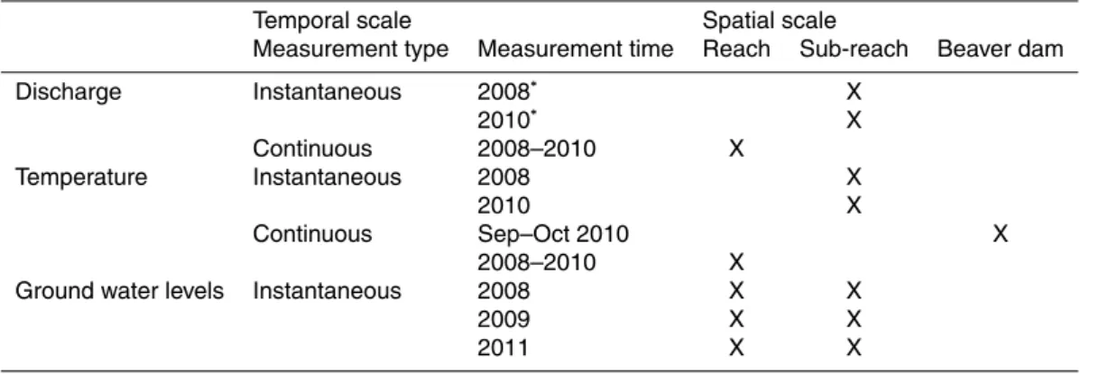
Table 1.Discharge, temperature and ground water level observations made at different spatial and temporal scales throughout the study reach.

Temporal scale Spatial scale

Measurement type Measurement time Reach Sub-reach Beaver dam

Discharge Instantaneous 2008∗ _X

2010∗ _X

Continuous 2008–2010 X

Temperature Instantaneous 2008 X

2010 X

Continuous Sep–Oct 2010 X 2008–2010 X

Ground water levels Instantaneous 2008 X X

2009 X X

2011 X X

(27)

HESSD

12, 839–878, 2015

M. Majerova et al.

Title Page

Tables Figures

◭ ◮

Back Close

Full Screen / Esc

Discussion

P

a

per

|

Discussion

P

a

per

|

Discussion

P

a

per

|

Discussion

P

a

per

|

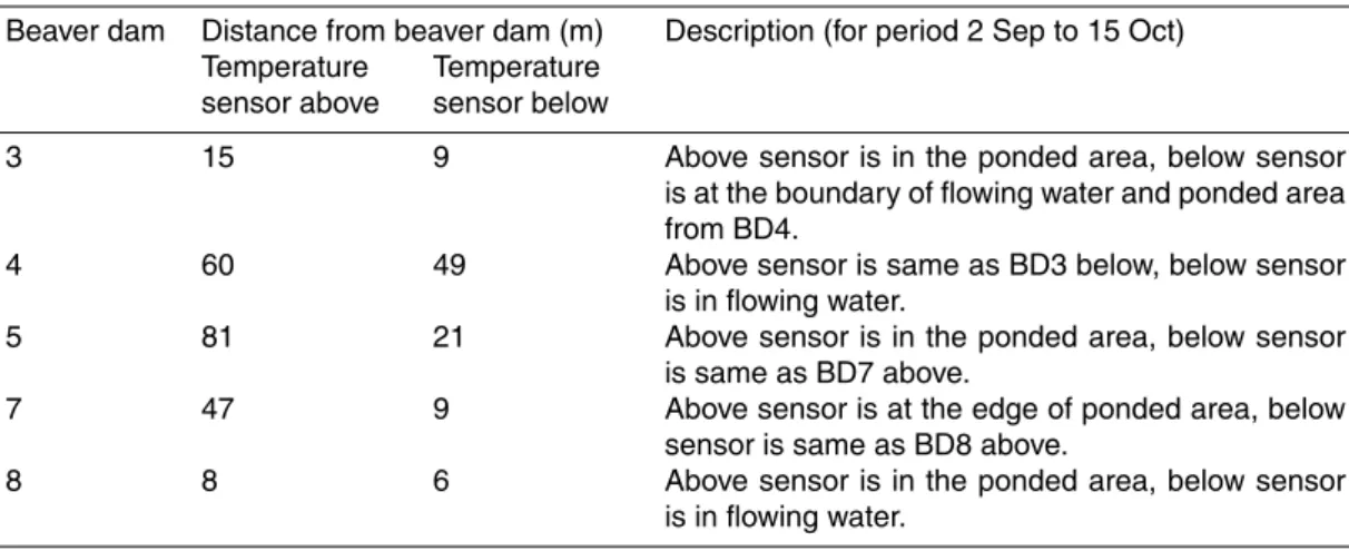
Table 2.Distance for temperature sensors located above and below individual beaver dams (BD) during 2 September to 15 October 2010 (Fig. 1).

Beaver dam Distance from beaver dam (m) Description (for period 2 Sep to 15 Oct) Temperature

sensor above

Temperature sensor below

3 15 9 Above sensor is in the ponded area, below sensor is at the boundary of flowing water and ponded area from BD4.

4 60 49 Above sensor is same as BD3 below, below sensor is in flowing water.

5 81 21 Above sensor is in the ponded area, below sensor is same as BD7 above.

7 47 9 Above sensor is at the edge of ponded area, below sensor is same as BD8 above.

(28)

HESSD

12, 839–878, 2015

M. Majerova et al.

Title Page

Tables Figures

◭ ◮

Back Close

Full Screen / Esc

Discussion

P

a

per

|

Discussion

P

a

per

|

Discussion

P

a

per

|

Discussion

P

a

per

|

Table 3.Change in flow (∆Q) and percent net change (%∆Q) for the study reach impacted by beaver dams (shown in Fig. 1) and for an adjacent, upstream control reach with no beaver dams present. Change in stream temperature (∆T), percent change (%∆T), and area of flowing water and ponded water area for the study reach impacted by beaver dams is listed as well. Change in flow and temperature and their percentages (∆Q, %∆Q,∆T, %∆T) were calculated as an average of daily∆values for each year (Figs. 3 and 5).

2008 2009 2010

Study reach (with beaver dams) _∆Q(L s−1

) ₋5.60 51.20 81.20

%∆Q 4.40 13.20 53.10

∆T (◦_C) _0.22 _0.17 _0.43

%∆T 2.10 1.10 4.40

Flowing water area (m2) 1776 – 1211

Ponded water area (m2) 0 – 2830

Water volume (m3) 636∗ _– ₂₄₄₉∗

Control reach (no beaver dams) ∆Q(L s−1

) 24.30 ₋55.90 ₋92.50

%∆Q ₋7.70 ₋19.80 ₋42.50

∗_{The water volume is an estimate from one-dimensional model where pre- and post-beaver dams flow}

(29)

HESSD

12, 839–878, 2015

M. Majerova et al.

Title Page

Tables Figures

◭ ◮

Back Close

Full Screen / Esc

Discussion

P

a

per

|

Discussion

P

a

per

|

Discussion

P

a

per

|

Discussion

P

a

per

|

Table 4.Sub-reach scale mean residence times for 2008 and 2010.

2008 2010

Sub-reach Stream distance Stream length Mean residence time Beaver Dam Mean residence time

(m) (m) (min) (min)

2 692 to 877 185 8 3, 4 36

3 877 to 995 118 4 5

4 995 to 1087 92 4.5 5 15

5 1087 to 1235 148 6.5 7, 8 29

6 1235 to 1291 56 4 4

(30)

HESSD

12, 839–878, 2015

M. Majerova et al.

Title Page

Tables Figures

◭ ◮

Back Close

Full Screen / Esc

Discussion

P

a

per

|

Discussion

P

a

per

|

Discussion

P

a

per

|

Discussion

P

a

per

|

(31)

HESSD

12, 839–878, 2015

M. Majerova et al.

Title Page

Tables Figures

◭ ◮

Back Close

Full Screen / Esc

Discussion

P

a

per

|

Discussion

P

a

per

|

Discussion

P

a

per

|

Discussion

P

a

per

|