The impact of large scale ionospheric structure on radio occultation retrievals

(1)

AMTD

4, 2525–2565, 2011

The impact of large scale ionospheric

structure

A. J. Mannucci et al.

Title Page

Abstract Introduction

Conclusions References

Tables Figures

◭ ◮

Back Close

Full Screen / Esc

Printer-friendly Version Interactive Discussion

Discussion

P

a

per

|

Dis

cussion

P

a

per

|

Discussion

P

a

per

|

Discussio

n

P

a

per

|

Atmos. Meas. Tech. Discuss., 4, 2525–2565, 2011 www.atmos-meas-tech-discuss.net/4/2525/2011/ doi:10.5194/amtd-4-2525-2011

Atmospheric Measurement Techniques Discussions

This discussion paper is/has been under review for the journal Atmospheric Measure-ment Techniques (AMT). Please refer to the corresponding final paper in AMT

if available.

The impact of large scale ionospheric

structure on radio occultation retrievals

A. J. Mannucci, C. O. Ao, X. Pi, and B. A. Iijima

Jet Propulsion Laboratory, California Institute Of Technology, MS 138-308, 4800 Oak Grove Drive, Pasadena, CA 91109, USA

Received: 26 February 2011 – Accepted: 10 March 2011 – Published: 4 May 2011 Correspondence to: A. J. Mannucci (tony.mannucci@jpl.nasa.gov)

(2)

AMTD

4, 2525–2565, 2011

structure

Title Page

Tables Figures

◭ ◮

Back Close

Full Screen / Esc

Discussion

P

a

per

|

Dis

cussion

P

a

per

|

Discussion

P

a

per

|

Discussio

n

P

a

per

Abstract

We study the impact of large-scale ionospheric structure on the accuracy of radio occul-tation (RO) retrievals of atmospheric parameters such as refractivity and temperature. We use a climatological model of the ionosphere as well as an ionospheric data assim-ilation model to compare quiet and geomagnetically disturbed conditions. The largest 5

contributor to ionospheric bias is physical separation of the two GPS frequencies as the GPS signal traverses the ionosphere and atmosphere. We analyze this effect in detail using ray-tracing and a full geophysical retrieval system. During quiet conditions, our results are similar to previously published studies. The impact of a major ionospheric storm is analyzed using data from the 30 October 2003 “Halloween” superstorm pe-10

riod. The temperature retrieval bias under disturbed conditions varies from 1 K to 2 K between 20 and 32 km altitude, compared to 0.2–0.3 K during quiet conditions. These results suggest the need for ionospheric monitoring as part of an RO-based climate observation strategy. We find that even during quiet conditions, the magnitude of re-trieval bias depends critically on ionospheric conditions, which may explain variations in 15

previously published bias estimates that use a variety of assumptions regarding large scale ionospheric structure. We quantify the impact of spacecraft orbit altitude on the magnitude of bending angle error. Satellites in higher altitude orbits (≧700 km) tend to have lower biases due to the tendency of the residual bending to cancel between the top and bottomside ionosphere. We conclude with remarks on the implications of this 20

study for long-term climate monitoring using RO.

1 Introduction

The Earth’s global climate is a subject of intense scientific and practical interest. The radio occultation remote sensing technique offers the possibility of precise and ac-curate atmospheric soundings that are well-suited for observing decadal-scale cli-25

(3)

AMTD

4, 2525–2565, 2011

structure

Title Page

Tables Figures

◭ ◮

Back Close

Full Screen / Esc

Discussion

P

a

per

|

Dis

cussion

P

a

per

|

Discussion

P

a

per

|

Discussio

n

P

a

per

|

parameters are retrieved based on a measurement of radio signal phase and phase rate. The fundamental measurement is therefore derived from signal timing, which is calibrated on-orbit to standards traceable to fundamental SI units.

Radio occultation uses a physically based retrieval scheme (Kursinski et al., 1996; Rocken et al., 1997) that permits detailed analyses of sources of measurement bias. 5

Such analyses are needed to ensure that measurement accuracy is absolutely cali-brated to the standard SI units. Detailed error analyses have been published (Kursin-ski et al., 1997; Hajj et al., 2002, 2004; Kuo et al., 2004; Steiner and Kirchengast, 2005) that analyze nearly all of the known error sources. For monitoring decadal-scale climate change, measurement bias should be less than∼0.1 K (Ohring et al., 2005; 10

Goody et al., 1998; Steiner et al., 2001), which motivates a reexamination of these past analyses that were focused initially on establishing precision of individual sound-ings at the level of∼1 K (Kursinski et al., 1997).

Recent studies that compare RO retrievals to other in-situ and remote methods, and simulation studies that consider various sources of measurement error, tend to confirm 15

the high accuracy of RO above the lower troposphere (Hajj et al., 2004; Kuo et al., 2005; Schreiner et al., 2007; Sun et al., 2010; Xu et al., 2009; He et al., 2009; Hayashi et al., 2009). The GPS RO technique achieves high accuracy by using “self-calibration”: data acquired during the measurement also serves to calibrate the observations. An example of self-calibration is the simultaneous tracking of a GPS “calibration satellite” 20

while the occulting satellite is tracked. The calibration satellite is a GPS satellite in view above the local spacecraft horizon. The additional satellite provides timing data that is combined with the occulting satellite data to remove receiver clock error from the retrieval. Thus, the retrieved atmospheric properties are not susceptible to receiver clock error.

25

Another form of self-calibration is used to reduce timing errors due to the Earth’s ionosphere and plasmasphere, a medium of tenuous plasma at altitudes between

(4)

AMTD

4, 2525–2565, 2011

structure

Title Page

Tables Figures

◭ ◮

Back Close

Full Screen / Esc

Discussion

P

a

per

|

Dis

cussion

P

a

per

|

Discussion

P

a

per

|

Discussio

n

P

a

per

refractive index introduces delay and delay rate to the GPS signal. Calibrating iono-spheric delay is accomplished by tracking the two GPS signal transmission frequen-cies: L1 (1.575 MHz) and L2 (1.228 MHz). The delay difference between the two fre-quencies is caused by the ionosphere. This difference can be calculated to high accu-racy using well-understood physical principles and formulas that describe the refractive 5

index dispersion of the ionospheric plasma. In contrast, the frequency dispersion of the neutral troposphere and stratosphere refractive index is negligible at GPS frequencies. Knowledge of the differential delay between L1 and L2 frequencies is used to calibrate precisely the ionospheric contribution.

Residual ionospheric calibration errors remaining after applying the dual-frequency 10

correction are not negligible for climate applications. The calibration is degraded by two factors. First, the L1 and L2 signal raypath trajectories through the ionosphere are not identical. The dual-frequency correction is incomplete if raypath separation is not accounted for. Fully accounting for raypath separation requires knowledge of electron density gradients along the raypath. Second, the refractive index gradient at 15

each frequency depends on Faraday rotation effects that depend on the magnetic field along the raypath, which is not accounted for in standard “first-order” calculations of ionospheric dispersion (so-called “higher-order” ionospheric effects. See Syndergaard, 2000; Vergados and Pagiatakis, 2010; Bassiri and Hajj, 1993).

In this paper, we present a detailed analysis of residual ionospheric calibration er-20

ror. We address the impact of raypath separation between the two GPS frequencies, caused by large-scale electron density gradient structures in the ionosphere. We per-form detailed ray-tracing calculations to analyze the occulting raypath geometries in realistic electron density structures using realistic transmitter-receiver geometries. The ionospheric electron density fields are obtained from global climatological and data 25

(5)

AMTD

4, 2525–2565, 2011

structure

Title Page

Tables Figures

◭ ◮

Back Close

Full Screen / Esc

Discussion

P

a

per

|

Dis

cussion

P

a

per

|

Discussion

P

a

per

|

Discussio

n

P

a

per

|

nature of the residual error in more detail. In Sect. 3 we discuss the analysis method and discuss the results in Sect. 4. A discussion of the results is included in Sect. 5.

2 Origins of ionospheric residual error

The Earth’s ionosphere is an ionized atmospheric medium containing a significant num-ber of free electrons primarily in the altitude range∼90–1200 km. At the transmission 5

frequencies of GPS, the refractive index (polarizability) of free electrons is far larger than that of neutral gas per unit mass. The refractive index of the daytime ionosphere at∼300 km altitude is comparable to the stratospheric refractive index at about∼20– 30 km altitude, although the densities of these two media differ by more than 10 orders of magnitude. Retrieving atmospheric properties requires calibration of ionospheric ef-10

fects on the signal, particularly for climate benchmark applications applied to the upper troposphere and stratosphere. In the mid-to-lower troposphere, residual refractivity or temperature errors due to ionosphere are less than 0.01% (Kursinski et al., 1997).

Accommodating ionospheric residual bias from a climate perspective is achieved by setting reliable upper bounds on that bias, and reducing the bias by algorithmic 15

and data processing approaches if possible. To achieve SI-traceable accuracy in the presence of uncertain electron density structure, robust upper bounds on residual error are needed so that all realistic ionospheric density configurations will result in residual errors less than the bound. We expect that very severe ionospheric storms that occur a few times per solar cycle may violate the upper bound. However, removing their impact 20

from climate averages is easily accomplished by monitoring ionospheric disturbance levels with widely available resources such as global GPS receiver networks.

Setting an upper bound on residual bias is achievable because of the physical na-ture of the RO retrieval process. Using physics-based simulation, we can calculate precisely the error in the atmospheric retrieval at a given altitude produced by a given 25

(6)

AMTD

4, 2525–2565, 2011

structure

Title Page

Tables Figures

◭ ◮

Back Close

Full Screen / Esc

Discussion

P

a

per

|

Dis

cussion

P

a

per

|

Discussion

P

a

per

|

Discussio

n

P

a

per

residual error. Implementing this approach is not trivial, and has not yet been imple-mented by the RO research community.

In the next sections, we describe the standard GPS approach to calibrating iono-spheric delays, and the causes of residual calibration bias. We then show the results of our study to quantify residual bias using simulation. Our analysis should be useful 5

to establishing SI-traceability in the presence of retrieval bias due to the ionosphere, at least for effects caused by large-scale ionospheric structure.

2.1 Dual frequency ionospheric correction

Ionospheric correction for GPS measurements is applied using the GPS data itself, by forming linear combinations of the carrier phase information at both transmission 10

frequencies. Geophysical observables derived from GPS radio occultation depend fundamentally on the measured Doppler shift at each GPS frequency, caused by re-fractive index variations from the neutral atmosphere and ionosphere. Differences in the Doppler shift between the two GPS frequencies are solely due to effects of the ionosphere. The physical basis by which Doppler shift varies with frequency is well 15

understood. Algorithms have been developed that use the measurements at both fre-quencies to create a new observable that is nearly free of ionospheric effects, thus creating an observable that depends only on the atmospheric refractive index (Hajj et al., 2002). The algorithms use the fact that, to first order, the phase delay incurred by the ionosphere is proportional to the inverse square of the signal frequency (1/f2). 20

Residual ionospheric error occurs because the phase delay is not exactly propor-tional to 1/f2. Two primary factors cause deviation from the 1/f2dependence. Faraday rotation effects due to the geomagnetic field introduce 1/f3(cubic) terms in the phase delay that depend on the geomagnetic field strength and electron density along the raypath. More significantly, spatial gradients of electron density cause the L1 and L2 25

(7)

AMTD

4, 2525–2565, 2011

structure

Title Page

Tables Figures

◭ ◮

Back Close

Full Screen / Esc

Discussion

P

a

per

|

Dis

cussion

P

a

per

|

Discussion

P

a

per

|

Discussio

n

P

a

per

|

as 1/f2. Deviation from 1/f2behavior depends in detail on the electron density structure of the ionosphere and the degree of separation along the occulting raypaths. Therefore, the magnitude of residual error varies with each occultation because of ionospheric variability or “weather”.

In the following paragraphs we describe an approach widely used to apply the iono-5

spheric correction to radio occultation data (Hajj et al., 2002). This approach is based on a procedure first suggested by Vorobev and Krasilnikova (1994). The dual frequency correction is applied to the bending angles at the L1 and L2 frequencies, interpolated to a common impact parameter, not to the phase delays themselves. (Bending angle is a by-product of the measured Doppler shift using geometrical considerations; see 10

Hajj et al., 2002). The impact parameter is the asymptotic distance of the rays from Earth’s center as they leave the atmosphere (see Hajj et al., 2002 for a definition). The bending angle approach largely compensates for the separation of L1 and L2 raypaths, and provides a more accurate correction than applying the correction to the measured GPS phase delays. The following linear combination of L1 and L2 bending angles 15

approximates the bending angle of the neutral atmosphere free of ionospheric effects:

αneut(a0)=C1α1(a0)−C2α2(a0) (1)

whereα1(a0) andα2(a0) are the bending angles at the L1 and L2 frequencies, respec-tively, at impact parametera0. The constantsC1 andC2 are functions of the two GPS frequenciesf1 andf2: C1=f

2 1/(f

2 1−f

2

2)≈2.545728, and C2=f 2 2/(f

2 1−f

2

2)≈1.545728. 20

Piecewise cubic interpolation of the bending angle versus impact parameter at each frequency is used to estimate the bending angle at the common impact parametera0. To reduce noise, an algebraic manipulation of this equation is formed as follows, using the fact thatC2=(C1−1):

αneut(a0)=α1(a0)+(C1−1)( ¯α1(a0)−α¯2(a0)) (2) 25

(8)

AMTD

4, 2525–2565, 2011

structure

Title Page

Tables Figures

◭ ◮

Back Close

Full Screen / Esc

Discussion

P

a

per

|

Dis

cussion

P

a

per

|

Discussion

P

a

per

|

Discussio

n

P

a

per

the high rate bending angleα1(a0) is computed approximately every 1/2 s based on the size of the Fresnel diameter (Hajj et al., 2002). The overall noise reduction com-pared to using completely unsmoothed angles is approximately a factor of 7. See also Sokoloksiy et al. (2009) for optimized filtering approaches.

The constantsC1and C2are the same as those used in the ionospheric correction 5

formula for phase delay and delay rate. The correction in Eq. (1) works very well if there is a linear relationship between bending angle and phase delay rate. Raypath separa-tion effects are reduced by interpolating to a common impact parametera0(Ladreiter and Kirchengast, 1996). Non-linearity in the relationship between bending angle and phase delay creates residual ionospheric error that is not accounted for in Eqs. (1) or 10

(2) (Gorbunov, 1996).

At altitudes below ∼10 km, due to atmospheric defocusing and reduction of signal amplitude, the L2 signal is often too weak for robust tracking (Hajj et al., 2002; Kuo et al., 2004; Mannucci et al., 2006). At such altitudes, Eq. (2) cannot be applied. In that case, the “smoothed” ionospheric correction terms in Eq. (2) are extrapolated 15

downward from higher altitudes to continue the ionospheric correction. The altitude range of the extrapolation is typically below 8–12 km as the second frequency is often lost at about 12 km altitude. A simulation study by Mannucci et al. (2006) suggests extrapolation may cause refractivity errors of ∼0.05% near the upper altitude range where the L2 loss first occurs.

20

The ionospheric calibration approach represented in Eqs. (1) and (2) is used in the simulated temperature and refractivity retrievals in this study. We also analyze bending angles directly for the L1 and L2 frequencies. For the bending angle results presented here, we apply the dual-frequency correction without interpolation to a common impact parameter. Thus, our bending angle residuals are somewhat larger than what ap-25

(9)

AMTD

4, 2525–2565, 2011

structure

Title Page

Tables Figures

◭ ◮

Back Close

Full Screen / Esc

Discussion

P

a

per

|

Dis

cussion

P

a

per

|

Discussion

P

a

per

|

Discussio

n

P

a

per

|

2.2 Residual ionospheric error: L1/L2 path separation and higher-order effects

The most significant source of ionospheric bias is that refractive index (electron den-sity) gradients along the raypath cause the L1 and L2 signals to follow different paths in the ionosphere (Syndergaard, 2000; Ladreiter and Kirchensgast, 1996). A dual-frequency correction of the form Eq. (1) cannot account for this raypath separation 5

since the refractive index gradients are not included in the formula. In this paper, we fo-cus exclusively on raypath separation. Higher order terms (Faraday rotation effect) are fully accounted for in the simulations presented here, since the full Appleton-Hartree formula for refractive index (e.g. Davies, 1990; Bassiri and Hajj, 1993) is used in the simulations, including a realistic representation of the Earth’s magnetic field (IGRF 10

model; see IAGA, 2003).

3 Approach

The propagation path of an electromagnetic wave through a medium such as the at-mosphere or ionosphere is determined by the refractive index variations in the vicinity of the path. The path deviates from straight-line propagation due to spatial gradients in 15

the refractive index near the path. Far from obstructions, the propagation pathr of the

wave’s energy is governed by the eikonal equation (Born and Wolf, 1980):

d d s(n(r)

dr

d s)=∇n(r) (3)

wheren(r)is the refractive index of the medium, assumed here to be dependent on

lo-cationr. The scalarsis the distance along the pathr. Ray-tracing is solving Eq. (3) for

20

the pathr(s) when the starting and ending points of the path are known. Ray-tracing

(10)

AMTD

4, 2525–2565, 2011

structure

Title Page

Tables Figures

◭ ◮

Back Close

Full Screen / Esc

Discussion

P

a

per

|

Dis

cussion

P

a

per

|

Discussion

P

a

per

|

Discussio

n

P

a

per

(2). Ray-tracing is not typically used in the retrieval process because it is far more computationally intensive than traditional methods.

We perform detailed ray-tracing studies through representative ionospheres to study the impact of ionospheric structure on RO retrievals. Ray-tracing permits us to examine how properties of ionospheric structure impact the retrieval accuracy. For example, 5

our study demonstrates that orbit altitude plays a role in the magnitude of residual ionospheric errors. We find that symmetric horizontal ionospheric structure about the raypath tangent point leads to smaller retrieval errors compared to highly asymmetric structures. Ray-tracing was used in Syndergaard et al. (2000) to validate the theoretical treatment of ionospheric residual found in that work.

10

Representative ionospheric electron density distributions are derived from two sources for this study: the International Reference Ionosphere (IRI) (Bilitza and Reinisch, 2008) and the Global Assimilative Ionosphere Model (GAIM) developed at JPL and the University of Southern California (Wang et al., 2004). IRI is a widely used climatological ionosphere model that provides values of electron density at any world-15

wide location specified by altitude, latitude and longitude. IRI uses as input the F10.7 index, as a proxy for solar radiation in the extreme ultraviolet and soft X-ray bands. The index is based on measurements of solar emittance at 10.7 cm wavelength. IRI electron density distributions represent how electron density varies with solar cycle and local time, two important factors that determine ionospheric variability. Studies using 20

IRI and other models suggest that residual ionospheric effects are largest near solar maximum daytime, but are negligible (<0.05 K) at nighttime and during solar minimum, from altitudes 25 km downward (Kursinski et al., 1997).

We use the Global Assimilative Ionosphere Model (GAIM) as an another source of electron density distribution. GAIM is used to analyze cases that deviate from average 25

(11)

AMTD

4, 2525–2565, 2011

structure

Title Page

Tables Figures

◭ ◮

Back Close

Full Screen / Esc

Discussion

P

a

per

|

Dis

cussion

P

a

per

|

Discussion

P

a

per

|

Discussio

n

P

a

per

|

GPS measurements and other systems to augment climatological or physics-based representations. Techniques such as GAIM have already shown great promise in im-proving upon climatology to produce three-dimensional maps of ionospheric electron density on global scales. We use GAIM assimilation runs during an extreme iono-spheric space weather event in 2003 to analyze residual ionoiono-spheric errors under ex-5

tremely unfavorable conditions. Input data for these runs is based on ground-based GPS receivers distributed globally, measuring total electron content above the receiver locations (Mannucci et al., 1998).

Previous research (Kursinski et al., 1997; Steiner et al., 2001) has shown that resid-ual ionospheric bias can approach 0.3 K at altitudes between 25–35 km during day-10

time solar maximum conditions. Recent research and theoretical work (Syndergaard, 2000) indicates that residual bias increases with electron density magnitudes, which are often controlled by the radiance level of the Sun at EUV and shorter wavelengths. Therefore, residual bias depends on the electron density magnitudes assumed. These magnitudes in turn depend on the assumed solar radiation environment. For a given 15

solar radiation environment and quiet geomagnetic conditions, electron density mag-nitudes can often deviate from climatological behavior by a factor of two (Brown et al., 1991). Variations of electron density near solar maximum daytime conditions must be accounted for to set reliable upper bounds on the level of ionospheric residual bias in retrievals.

20

Ionospheric storms, which are byproducts of geomagnetic activity, can increase iono-spheric residuals significantly compared to quiet geomagnetic conditions. The residual bias increases for two reasons that often occur simultaneously during storms: overall electron density values increase as do their spatial gradients. According to Eq. (3), the raypaths followed at the L1 and L2 frequencies depend on refractive index magnitudes 25

and spatial gradients. Separation of raypaths between L1 and L2 generally increases under both density increases and gradient increases for fixed density.

(12)

AMTD

4, 2525–2565, 2011

structure

Title Page

Tables Figures

◭ ◮

Back Close

Full Screen / Esc

Discussion

P

a

per

|

Dis

cussion

P

a

per

|

Discussion

P

a

per

|

Discussio

n

P

a

per

when the ionospheric residuals are largest. Simulations for nighttime and solar min-imum are not considered. We show in detail which part of the ionospheric electron density profile is cause for greatest raypath separation.

4 Results

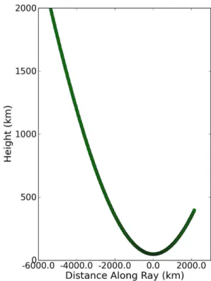
A representative occultation raypath has been selected for detailed study in these sim-5

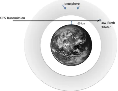
ulation experiments. The minimum altitude of the raypath (tangent point) is 60 km. At such high altitudes, ionospheric residuals have the largest impact on retrieval error. The goal of achieving temperature biases less than 0.1 K is unrealistic at 60 km and higher altitudes, limiting the possibility of using radio occultation in applications where SI-traceability is desired at such high altitudes. At lower altitudes, atmospheric bending 10

dominates and the impact of ionospheric residuals is less.

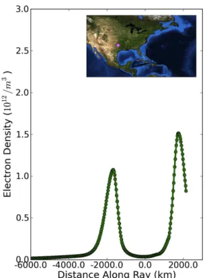
We use a representative ray-path from an actual occultation acquired by the CHAMP satellite on 30 October 2003. The altitude of the ray versus distance from the tangent point (ray perigee) is shown in Fig. 1. The location of the raypath tangent point is shown as the inset in Fig. 2. A severe geomagnetic storm was in progress on 30 Oc-15

tober 2003. Very large ionospheric total electron content and electron density spatial gradients were detected by a ground-based GPS receiver network in the vicinity of the occultation ray-path (for details, see Mannucci et al., 2005). This particular occultation geometry was selected to coincide with extreme ionospheric conditions as represented by the GAIM.

20

(13)

AMTD

4, 2525–2565, 2011

structure

Title Page

Tables Figures

◭ ◮

Back Close

Full Screen / Esc

Discussion

P

a

per

|

Dis

cussion

P

a

per

|

Discussion

P

a

per

|

Discussio

n

P

a

per

|

4.1 Results using the International Reference Ionosphere

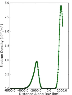
The IRI-95 model was run for 30 October 2003. The F10.7 solar flux index on that day was 267 (adjusted value), a very high value exceeding by ∼48% the average F10.7 value during solar maximum years 2000–2001. The electron density encoun-tered along the raypath is shown in Fig. 2. The two-peak structure is a result of twice 5

entering and exiting the ionospheric “annulus”, as shown schematically in Fig. 3. In Fig. 2, the electron densities for the L1 and L2 paths di_ffer imperceptibly despite the slightly different raypaths and do not show on this figure. The two electron density peak values occur when the raypath is traversing altitudes 260 and 250 km, near the altitudes of peak electron density in the model (see right panel, Fig. 15, for vertical 10

electron density profiles from the IRI-95 output near the tangent point). Densities were linearly extrapolated downward from altitudes of 100 km since the model run cuts off abruptly at that altitude. For this study, we use an occultation raypath from an actual CHAMP orbit when the satellite altitude was 400 km. We will show later that the altitude of the receiver has an impact on the magnitude of the ionospheric residual bias. 15

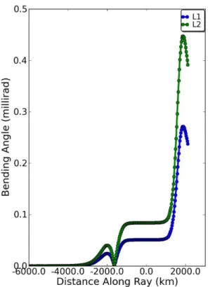
The accumulated bending angle along the raypath for the L1 and L2 frequencies is shown in Fig. 4. The bending angle is with respect to the direction that the raypath leaves the transmitter. The angle differs significantly between the two frequencies be-cause of the frequency-dependent refractive index according to the 1/f2law. The accu-mulated bending angle follows a similar overall pattern for the two frequencies. Several 20

features are notable. Near−1300 km, the accumulated bending angle approaches very low values. At this point along the raypath, the positive bending due to the topside iono-sphere is nearly compensated for by the negative bending in the bottomside, yielding a small net bending value. Shortly after this minimum, the raypath drops below 100 km, effectively exiting the ionosphere. The bending angle increases slowly due to the resid-25

(14)

AMTD

4, 2525–2565, 2011

structure

Title Page

Tables Figures

◭ ◮

Back Close

Full Screen / Esc

Discussion

P

a

per

|

Dis

cussion

P

a

per

|

Discussion

P

a

per

|

Discussio

n

P

a

per

bending angle direction begins to reverse again. The net bending angle at the receiver is∼0.13 millirad for the L1 frequency, reached at∼2200 km.

The retrieval of geophysical parameters depends on the accumulated bending angle at the location of the GPS receiver, which is generally orbiting at a radius within the ionosphere. Since the accumulated bending angle does not increase monotonically, 5

certain altitudes for the GPS receiver are more favorable for obtaining low residual biases. For this example, altitudes near 195 km yield zero bending angle due to can-cellation from the topside and bottomside. The altitude of this complete cancan-cellation will vary with electron density distribution. More generally (and realistically), higher altitudes above the F2 peak density (above 500 km) will result in more cancellation of 10

the accumulated bending, as can be seen by the bending angle trends near the end of the raypath in Fig. 4. The reduced residual ionosphere at higher altitudes is further discussed in Sect. 4.3.

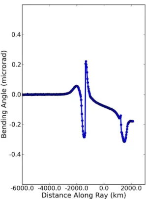
The linear combination of bending angles at the L1 and L2 frequencies (Eq. 1) pro-duces an estimate of bending caused solely by the neutral atmosphere. Electron den-15

sity gradients along the L1 and L2 raypaths result in imperfect cancellation of iono-spheric effects when this formula is applied. In Fig. 5, we plot the residual bending angle calculated from our ray-tracing simulation, assuming the dual-frequency correc-tion is applied. In the absence of ray-path separacorrec-tion, the residual bending should be zero for all points along the raypath. Deviations from zero in Fig. 5 are a measure of 20

ionospheric residual due to raypath separation. The residual bending changes rapidly as the raypath enters and exits the first ionospheric traversal. On exiting the iono-sphere, the residual bending remains nearly constant with a small bias of∼ −1×10−7 radians. The structure of the ionosphere results in a fortuitous cancellation of bend-ing angle from the top and bottomsides, as discussed before. Bendbend-ing angle residual 25

(15)

AMTD

4, 2525–2565, 2011

structure

Title Page

Tables Figures

◭ ◮

Back Close

Full Screen / Esc

Discussion

P

a

per

|

Dis

cussion

P

a

per

|

Discussion

P

a

per

|

Discussio

n

P

a

per

|

error. If the receiver were at higher altitude, bending cancellation would occur similarly to what occurs in the first ionospheric traversal, reducing the overall impact of the iono-sphere on the retrieval. The impact of satellite altitude is discussed later for a low-Earth orbiter (LEO) at COSMIC altitudes (780 km versus 400 km for CHAMP).

4.2 Global assimilative ionosphere model – major ionospheric storm

5

We use the GAIM to assess the impact of “worst-case” electron density gradients that occur during geomagnetic storms, conditions that are not generally captured by the IRI. Plots analogous to those just described for IRI are Figs. 6–8. The raypath geom-etry is identical in the two cases. The GAIM assimilates total electron content (TEC) data from the global network of Global Positioning System (GPS) ground receivers and 10

thus captures, at least approximately, horizontal electron gradients and magnitudes that occurred during the storm. The GPS TEC data captures storm conditions that occurred on 30 October 2003. The storm is characterized by large TEC daytime val-ues, enhanced spatial gradients and vertical “uplift” of electron density as reported in Mannucci et al. (2005).

15

The GAIM estimates confirm that electron densities reach larger magnitudes com-pared to quiet time. Electron densities differ significantly between the entering and exit phases of the trans-ionospheric propagation (Fig. 6). Peak electron density in the entrance lobe of the ionosphere is slightly lower than IRI in the storm-time case repre-sented by GAIM. In the exit lobe, the peak electron density is a factor of 1.75 larger in 20

the storm case compared to IRI. Bending angle (Fig. 7) for the storm case is similarly larger in the exit lobe compared to the entrance lobe.

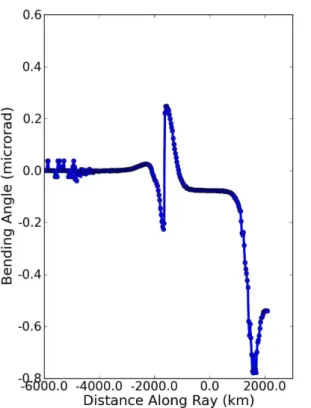
Residual bending angle after correction for the storm case is shown in Fig. 8. The residual follows a similar functional form for the IRI case. The bending angle affecting the retrieval is the value at the receiver location at the ray end-point. This final value is 25

(16)

AMTD

4, 2525–2565, 2011

structure

Title Page

Tables Figures

◭ ◮

Back Close

Full Screen / Esc

Discussion

P

a

per

|

Dis

cussion

P

a

per

|

Discussion

P

a

per

|

Discussio

n

P

a

per

are a significant contributing factor to the increased residual beyond the overall scalar increase in electron density associated with the storm.

4.3 Spacecraft orbit considerations

The orbital altitude of the GPS receiver is a significant factor determining the mag-nitude of the ionospheric residual. The analysis of the previous section shows that 5

ionospheric bending in the topside ionosphere is of opposite sense to bending in the bottomside, leading to partial cancellation. The degree of cancellation depends on spacecraft altitude. The analysis just concluded is performed for a spacecraft at the CHAMP altitude of 400 km. We have also computed residual ionospheric e_ffects for a LEO at 780 km altitude, corresponding to the final altitude of the COSMIC satellites. 10

See Sydergaard (2000) for comments related to orbit altitude.

Figure 9 shows the electron density along an occultation ray-path for the storm day, GAIM case, assuming a spacecraft at COSMIC altitude of 780 km (versus 400 km for CHAMP). The COSMIC raypath tangent point is at approximately the same location as CHAMP (within 1◦), but the orientation is ₊233◦ with respect to North. For CHAMP, 15

the orientation angle is+137◦. Orientation angle affects the electron density gradients encountered along the raypath, which could differ significantly for these two orientation angles during the disturbed conditions studied here.

The COSMIC altitude is significantly above the altitude of peak electron density (∼400 km). The electron density traces for the entrance and exit lobes now show simi-20

lar structure. For both lobes, the electron density is approximately symmetric about the peak. Bending cancellation will be more complete between bottomside and topside. In the comparable CHAMP case (Fig. 6), the electron density at the receiver is close to the peak value at the exit lobe. Bending that occurs on the bottomside is not cancelled by bending on the topside. The resulting ionospheric residual bending for the COSMIC 25

(17)

AMTD

4, 2525–2565, 2011

structure

Title Page

Tables Figures

◭ ◮

Back Close

Full Screen / Esc

Discussion

P

a

per

|

Dis

cussion

P

a

per

|

Discussion

P

a

per

|

Discussio

n

P

a

per

|

compared to the peak bending. The difference in bending angle between COSMIC and CHAMP is due to the differing link orientations, resulting in different electron den-sity gradients along the path. In the CHAMP case, the residual bending angle at the receiver location is 65% of its peak value, versus only 35% of the peak in the COSMIC case.

5

4.4 Retrieval error

The case studies in Sections 4.1–4.3 illustrate the detailed dependence of ionospheric residual on ionospheric structure and raypath geometry. In this section, we perform an end-to-end simulation to calculate the error in temperature retrieval due to the iono-spheric residual. We perform a full ray-trace calculation through both the ionosphere 10

and atmosphere and generate simulated data for use in the retrieval algorithm, apply-ing the bendapply-ing angle correction as described in Eqs. (1) and (2).

The end-to-end simulation system is diagrammed in Fig. 11. Ray-tracing is per-formed separately for the L1 and L2 signal paths that are propagated to a simulated receiver location at 400 km altitude. As described above, the IRI or GAIM electron 15

density models were used for the ionospheric ray-tracing calculation. A spherically-symmetric (radial dependence only) refractivity profile from ECMWF was used for the atmospheric ray-trace calculation, representative of conditions on 31 October 2003 near the occultation tangent point at 0 UTC (the exact profile used is not relevant to the analysis). The standard retrieval process is then performed on L1 and L2 phases af-20

ter perfect subtraction of geometrical distances and assuming perfectly known clocks. After calculation of bending angle at each frequency, the standard ionospheric dual-frequency correction is applied to the bending angles interpolated to common impact parameter (Eq. 1). The retrieved atmospheric refractivity and temperature profiles are differenced with the input refractivity and temperature profile. The net result is an esti-25

(18)

AMTD

4, 2525–2565, 2011

structure

Title Page

Tables Figures

◭ ◮

Back Close

Full Screen / Esc

Discussion

P

a

per

|

Dis

cussion

P

a

per

|

Discussion

P

a

per

|

Discussio

n

P

a

per

study to altitudes greater than 20 km, since below that altitude the ionospheric residual decreases rapidly.

Simulation results are shown in Fig. 12, assuming the electron density along the oc-culting raypath is given by the IRI model. The raypath geometry is the same as used for the CHAMP case studies (for example, Figs. 1 and 2). To retrieve temperature, the 5

simulation needs a pressure value at 40 km to initialize the hydrostatic integral (Hajj et al., 2002). This initial value is supplied at 40 km altitude, resulting in zero temper-ature error at this altitude. Figure 12 plots the tempertemper-ature bias due to ionosphere residual as calculated using ray-tracing, ignoring other sources of error. Refractivity bias is shown in Fig. 13, which requires no initialization and therefore grows without 10

limit as altitude increases. The reason for altitude growth in refractivity bias is that the ionospheric residual remains relatively constant with altitude, whereas the atmospheric signal decreases rapidly with altitude. The net result is larger retrieval bias due to the ionospheric residual as altitude increases. Random error also increases with altitude, an effect which is not included in this simulation.

15

Temperature errors in the range∼0.2–0.3 K between 20–30 km altitudes are evident in Fig. 12 for both the stormy and quiet IRI cases analyzed. The quiet IRI case cor-responds to 27 October 2003, a geomagnetically quiet day preceding the storms on 29–30 October 2003. The two cases are nearly identical because IRI is run in a mode that does not ingest data or adjust the model based on storminess. Therefore, the 20

IRI electron density profiles are nearly the same for the two days, resulting in nearly identical residual error. In both cases, the temperature bias is close to the value of 0.3 K reported by Kursinski et al. (1997) at 25 km altitude for solar maximum daytime conditions. Kursinki et al. (1997) used 1-D raytracing through a Chapman layer rather than the higher-fidelity IRI three-dimensional model used here. The temperature error 25

(19)

AMTD

4, 2525–2565, 2011

structure

Title Page

Tables Figures

◭ ◮

Back Close

Full Screen / Esc

Discussion

P

a

per

|

Dis

cussion

P

a

per

|

Discussion

P

a

per

|

Discussio

n

P

a

per

|

Although the storm mode for IRI might produce somewhat more realistic results, climatological models in general are not well suited to capturing storm conditions. Our Global Assimilative Ionosphere Model (GAIM) results are shown in Fig. 14 for the storm day and for a quiet day preceding the storm (27 October 2003). Storm-time differences are clear due to the larger electron density gradients during the storm. The temperature 5

bias due to the geomagnetic storm reaches 1.5 K at 25 km compared to∼0.3 K for the quiet case.

The ionospheric storm of 30 October 2003 is an extreme case producing large elec-tron density gradients and magnitudes during daytime. Such large storms typically occur only a few times per 11-year solar cycle (generally during the declining phase 10

of the cycle). It is instructive to consider their impact on the retrieval although such storms do not pose practical problems for radio occultation measurements used for climate monitoring. The presence of large storms is easily detected and removed from climate averages with negligible e_ffect. This study suggests that monitoring space weather conditions is important and that during severely disturbed conditions, atmo-15

spheric variables from RO such as temperature and pressure should be excluded from climatological averages.

It is also useful to consider the impact of electron density variation on the retrieval accuracy, apart from extreme storm conditions. Variable solar insolation (X-ray and ex-treme ultraviolet wavelengths) and local “ionospheric weather” factors modulate elec-20

tron densities during nominal conditions also. Such modulation can reach factors of two during daytime conditions (Brown et al., 1991). We analyze the case where the quiet-time IRI densities are doubled, to approximately examine the effect of quiet-time variability. Varying electron density by scaling provides some insight into ways that electron density magnitude may be affecting the results of different simulations appear-25

(20)

AMTD

4, 2525–2565, 2011

structure

Title Page

Tables Figures

◭ ◮

Back Close

Full Screen / Esc

Discussion

P

a

per

|

Dis

cussion

P

a

per

|

Discussion

P

a

per

|

Discussio

n

P

a

per

Figure 15 illustrates dependence of retrieval error on electron density magnitude. Three retrieval simulations are compared: quiet IRI (as in Fig. 12), quiet GAIM (as in Fig. 14), and doubled IRI electron densities. This last case shows the impact of scaling electron density without creating the anomalous electron density gradients that occur during a major storm. The right panel of Fig. 15 shows the electron density profiles near 5

the occultation tangent point for these three cases (34◦N, 98◦W). The left panel shows the retrieval bias in temperature units. The qualitative result from these cases suggests that larger electron peak densities lead to larger residuals, a direct result of the larger bending that occurs overall. (See Syndergaard, 2000 for a theoretical discussion of this point). Therefore, in understanding previously published results that estimate the 10

influence of ionospheric residual on retrieval bias, it is important to carefully specify the electron density values used to reach those results. Factors-of-two differences in peak electron densities are observed between differing models or between the same model at di_fferent times, even at the same phase in the solar cycle.

5 Discussion

15

This analysis shows that details of the electron density distribution and orbit altitude are two major factors determining retrieval biases that occur due to ionospheric resid-ual, affecting upper troposphere and lower stratosphere atmospheric retrievals. Iono-spheric residual is sensitive to spacecraft altitude because the vertical distribution of ionospheric electron density reaches a peak near orbital altitudes of low Earth orbiting 20

receivers. Residual error accumulated as rays traverse the bottom side ionosphere be-low the peak density tend to cancel residual error of opposite sign as the ray traverses the topside above the peak. For spacecraft near the peak electron density altitude, such as CHAMP (∼400 km), there is minimal topside/bottomside cancellation.

We have for the first time used an ionospheric data assimilation model to as-25

(21)

AMTD

4, 2525–2565, 2011

structure

Title Page

Tables Figures

◭ ◮

Back Close

Full Screen / Esc

Discussion

P

a

per

|

Dis

cussion

P

a

per

|

Discussion

P

a

per

|

Discussio

n

P

a

per

|

“Halloween Storms” of 29–30 October 2003. For long-term climate applications of GPS data, it is important to remove such active periods from climatological averages. The number of such excised days is likely to be insignificant if only the most extreme events are considered, which typically last 1–2 days and occur perhaps 5–10 times per 11 yr solar cycle. Further research is needed to understand how the full spectrum of 5

ionospheric disturbances can affect the residual error during the declining phase of the solar cycle, since it is likely that moderately disturbed conditions have an impact also. We note that recent solar-terrestrial research shows that during the declining phase of the solar cycle moderately active conditions can persist for days to weeks. These long-duration, mild geomagnetic conditions are due to the presence of coronal holes, 10

which appear during the declining phase (Tsurutani et al., 2006).

This study generally agrees with past efforts in characterizing the magnitude of the ionospheric residual on retrieval error. However, there is a spread in past research likely due to the detailed assumptions used regarding ionospheric structure. We believe that even at 20 km altitude, ionospheric residual remains too large for climate monitoring 15

applications during daytime solar maximum conditions. Although past studies may cor-rectly conclude that RO is ready for observing long-term climate (Steiner et al., 2001; Steiner et al., 2009), we believe “the margin for error” is too narrow and should be increased. Continuing efforts are encouraged to develop algorithms that reduce the ionospheric residual error using improved algorithms and techniques (Ladreiter and 20

Kirchengast, 1996; Gorbunov et al., 1996; Syndergaard, 2000). As discussed by Gor-bunov et al. (1996) the bending angle correction formula (Eq. 1) implicitly relies on a linear relationship between bending angle and phase delay due to the ionosphere. Such linearity is violated by raypath separation and non-spherical symmetry of iono-spheric structure. Clearly there are opportunities for robust correction algorithms that 25

improve upon Eq. (1).

(22)

AMTD

4, 2525–2565, 2011

structure

Title Page

Tables Figures

◭ ◮

Back Close

Full Screen / Esc

Discussion

P

a

per

|

Dis

cussion

P

a

per

|

Discussion

P

a

per

|

Discussio

n

P

a

per

of the current study since neither the IRI nor GAIM models reproduce them effectively. Fortunately, for climate applications the presence of these structures generally pro-duces distinct fluctuations in the data, so that mitigating strategies can be devised. Further work is needed to characterize the frequency and distribution of such struc-tures in the context of global climate monitoring.

5

It is likely that long-term climate records will combine a mix of RO satellites orbiting at varying altitudes. Our analysis shows a significant impact of orbit altitude on the magnitude of ionospheric residual bending. Therefore, care must be exercised when creating the long-term record, to avoid small systematic biases that might vary with mission. Clearly, this matter is tied to the overall question of reducing ionospheric 10

residuals to achieve greater margin for error in forming climate averages from RO data. As part of this margin, we recommend that ionospheric activity indices be consulted to make sure that increased ionospheric activity is not affecting the record.

6 Conclusion

We have performed a detailed propagation study for GPS signals in an occulting geom-15

etry to gain insight into the sources of residual ionospheric bias affecting upper tropo-sphere/lower stratospheric retrievals. We focused on the separation of the raypaths at the two GPS frequencies as the physical basis for the ionospherc residual bias after ap-plying the usual dual-frequency correction. This is the first study to address the case of severe geomagnetic storms that create large electron density magnitudes and spatial 20

gradients in the ionosphere. The large resulting retrieval bias suggests that monitoring ionospheric conditions is a necessary prerequisite for long-term climate observation with RO, to excise those periods from the record where the level of ionospheric distur-bance is unacceptably high.

We find also that orbit altitude affects the bias, potentially in a significant amount 25

(23)

AMTD

4, 2525–2565, 2011

structure

Title Page

Tables Figures

◭ ◮

Back Close

Full Screen / Esc

Discussion

P

a

per

|

Dis

cussion

P

a

per

|

Discussion

P

a

per

|

Discussio

n

P

a

per

|

must be exercised to account for possible bias differences when forming long-term climate averages using multiple satellite time series of data.

The way forward for climate monitoring applications is to develop a strategy for set-ting robust upper bounds to ionospheric residual bias under a wide variety of solar and geomagnetic conditions. This upper bound is the means by which RO retrievals can 5

maintain SI-traceability in the presence of ionospheric effects. Given the size of the bias above 25 km, it is highly desirable to develop ionospheric correction algorithms that are more accurate and robust than the standard dual-frequency bending angle correction. Even with improved algorithms, there will be disturbances for which the residual bias is unacceptably large and in such cases the RO retrievals should not be 10

included in long-term climate averages. This implies that some form of space weather monitoring should be implemented as part of the climate observation strategy, to en-sure that disturbed conditions do not play a disproportionately large role in the climate averages.

Acknowledgements. The research for this paper was performed at the Jet Propulsion Labora-15

tory, California Institute of Technology under contract with NASA. The authors wish to acknowl-edge support of the NASA Earth Science Directorate.

References

Bassiri, B. and Hajj, G.: Higher-order ionospheric e_ffects on the global positioning system observables and means of modeling them, Manuscripta Geodaetica, 18, 280–289, 1993. 20

Bilitza, D. and Reinisch, B. W.: International Reference Ionosphere 2007: Improvements and new parameters, Adv. Space Res., 42, 599–609, doi:10.1016/j.asr.2007.07.048, 2008. Born, M., and Wolf, E., Principles of Optics: Electromagnetic Theory of Propagation,

Interfer-ence and Diffraction of Light, 6th Edition, Pergamon, Elmsford, NY, 1980.

Brown, L. D., Daniell, R. E., Fox, M. W., Klobuchar, J. A., and Doherty, P.H.: Evaluation of 6 25

ionospheric models as predictors of total electron-content, Radio Science, 26, 1007–1015, 1991.

(24)

AMTD

4, 2525–2565, 2011

structure

Title Page

Tables Figures

◭ ◮

Back Close

Full Screen / Esc

Discussion

P

a

per

|

Dis

cussion

P

a

per

|

Discussion

P

a

per

|

Discussio

n

P

a

per

Gobiet, A. and Kirchengast, G.: Advancements of Global Navigation Satellite System radio oc-cultation retrieval in the upper stratosphere for optimal climate monitoring utility, J. Geophys. Res.-Atmos., 109, D24110, doi:10.1029/2004jd005117, 2004.

Goody, R., Anderson, J., and North, G.: Testing climate models: An approach, Bulletin of the American Meteorological Society, 79, 2541–2549, 1998.

5

Gorbunov, M. E., Sokolovsky, S. V., and Bengtsson, L.: Space refractive tomography of the atmosphere: Modeling of direct and inverse problems, Rep. Max Planck Inst for Meteorol., No. 210-59, Hamburg, Germany, 1996.

Hajj, G. A., Kursinski, E., R., Romans, L. J., Bertiger, W. I., and Leroy, S. S.: A technical description of atmospheric sounding by GPS occultation, J. Atmos. Sol.-Terr. Phy., 64, 451– 10

469, 2002.

Hardy, K. R., Hajj, G. A., and Kursinski, E. R.: Accuracies of atmospheric profiles obtained from GPS occultations, Int. J. Satell. Co., 12, 463–473, 1994.

Hayashi, H., Furumoto, J. I., Lin, X. N., Tsuda, T., Shoji, Y., Aoyama, Y., and Murayama Y.: Validation of Refractivity Profiles Retrieved from FORMOSAT-3/COSMIC Radio Occultation 15

Soundings: Preliminary Results of Statistical Comparisons Utilizing Balloon-Borne Observa-tions, Terr. Atmos. Ocean. Sci., 20, 51–58, doi:10.3319/tao.2008.01.21.01(f3c), 2009. He, W. Y., Ho, S. P., Chen, H. B., Zhou, X. J., Hunt, D., and Kuo, Y. H.:

Assess-ment of radiosonde temperature measureAssess-ments in the upper troposphere and lower stratosphere using COSMIC radio occultation data, Geophys. Res. Lett., 36, L17807, 20

doi:10.1029/2009gl038712, 2009.

International Association of Geomagnetism and Aeronomy (IAGA), D. V., Working Group 8: The 9th Generation International Geomagnetic Reference Field, Earth Planets and Space, 55, i-ii, 2003.

Kuo, Y. H., Schreiner, W. S., Wang, J., Rossiter, D. L., and Zhang, Y.: Comparison of 25

GPS radio occultation soundings with radiosondes, Geophys. Res. Lett., 32, L05817, doi:10.1029/2004gl021443, 2005.

Kuo, Y. H., Wee, T. K., Sokolovskiy, S., Rocken, C., Schreiner, W., Hunt, D., and Anthes, R. A.: Inversion and error estimation of GPS radio occultation data, J. Meteorol. Soc. Jpn., 82, 507–531, 2004.

30

(25)

AMTD

4, 2525–2565, 2011

structure

Title Page

Tables Figures

◭ ◮

Back Close

Full Screen / Esc

Discussion

P

a

per

|

Dis

cussion

P

a

per

|

Discussion

P

a

per

|

Discussio

n

P

a

per

|

positioning system, Science, 271, 1107–1110, 1996.

Kursinski, E. R., Hajj, G. A., Schofield, J. T., Linfield, R. P., and Hardy, K. R.: Observing Earth’s atmosphere with radio occultation measurements using the Global Positioning System, J. Geophys. Res.-Atmos., 102, 23429–23465, 1997.

Ladreiter, H. P. and Kirchengast, G.: GPS/GLONASS sensing of the neutral atmosphere: 5

Model-independent correction of ionospheric influences, Radio Science, 31, 877–891, 1996. Mannucci, A. J., Ao, C. O., Yunck, T. P., Young, L. E., Hajj, G. A., Iijima, B. A., Kuang, D.,

Mee-han, T. K., and Leroy, S. S.: Generating climate benchmark atmospheric soundings using GPS occultation data, SPIE Proceedings, 6301, 630108, doi:10.1117/12.683973, 2006. Mannucci, A. J., Tsurutani, B. T., Iijima, B. A., Komjathy, A., Saito, A., Gonzalez, W. D., 10

Guarnieri, F. L., Kozyra, J. U., and Skoug S.: Dayside global ionospheric response to the major interplanetary events of October 29–30, 2003 “Halloween storms”, Geophys. Res. Lett., 32, L12S02, doi:10.1029/2004gl021467, 2005.

Mannucci, A. J., Wilson, B. D., Yuan, D. N., Ho, C. H., Lindqwister, U. J., and Runge T. F.: A global mapping technique for GPS-derived ionospheric total electron content measurements, 15

Radio Science, 33, 565–582, 1998.

Ohring, G., Wielicki, B., Spencer, R., Emery, B., and Datla, R.: Satellite instrument calibration for measuring global climate change – Report of a Workshop, B. Ame. Meteorol. Soc., 86, 1303–1313, 2005.

Rocken, C., Anthes R., Exner M., Hunt, D., Sokolovskiy, S., Ware, R., Gorbunov, M., Schreiner, 20

W., Feng, D., Herman, B., Kuo, Y.H., and Zou, X.: Analysis and validation of GPS/MET data in the neutral atmosphere, J. Geophys. Res.-Atmos., 102, 29849–29866, 1997.

Schreiner, W., Rocken, C., Sokolovskiy, S., Syndergaard, S., and Hunt, D.: Estimates of the pre-cision of GPS radio occultations from the COSMIC/FORMOSAT-3 mission, Geophys. Res. Lett., 34, L04808, doi:10.1029/2006gl027557, 2007.

25

Sokolovskiy, S., Schreiner, W., Rocken, C., and Hunt, D.: Optimal Noise Filtering for the Iono-spheric Correction of GPS Radio Occultation Signals, J. Atmos. Ocean. Technol., 26, 1398– 1403, doi:10.1175/2009jtecha1192.1, 2009.

Steiner, A. K. and Kirchengast, G.: Error analysis for GNSS radio occultation data based on ensembles of profiles from end-to-end simulations, J. Geophys. Res.-Atmos., 110, D15307, 30

doi:10.1029/2004JD005251, 2005.

(26)

AMTD

4, 2525–2565, 2011

structure

Title Page

Tables Figures

◭ ◮

Back Close

Full Screen / Esc

Discussion

P

a

per

|

Dis

cussion

P

a

per

|

Discussion

P

a

per

|

Discussio

n

P

a

per

Geod., 26, 113–124, 2001.

Steiner, A. K., Kirchengast, G., Lackner, B. C., Pirscher, B., Borsche, M., and Foelsche, U.: Atmospheric temperature change detection with GPS radio occultation 1995 to 2008, Geo-phys. Res. Lett., 36, L18702, doi:10.1029/2009gl039777, 2009.

Steiner, A. K., Kirchengast, G., and Ladreiter, H. P.: Inversion, error analysis, and validation of 5

GPS/MET occultation data, Ann. Geophys.-Atmos. Hydrospheres Space Sci., 17, 122–138, 1999.

Sun, B. M., Reale, A., Seidel, D. J., and Hunt, D. C.: Comparing radiosonde and COSMIC atmospheric profile data to quantify differences among radiosonde types and the effects of imperfect collocation on comparison statistics, J. Geophys. Res.-Atmos., 115, D23104, 10

doi:10.1029/2010jd014457, 2010.

Syndergaard, S.: On the ionosphere calibration in GPS radio occultation measurements, Radio Science, 35, 865–883, 2000.

Tsurutani, B. T., Gonzalez, W. D., Gonzalez, A. L. C., Guarnieri, F. L., Gopalswamy, N., Grande, M., Kamide, Y., Kasahara, Y., Lu, G., Mann, I., McPherron, R., Soraas, F., and Vasyliunas, 15

V.: Corotating solar wind streams and recurrent geomagnetic activity: A review, J. Geophys. Res-Space Phys., 111, A07S01, doi:10.1029/2005JA011273, 2006.

Vergados, P. and Pagiatakis, S. D.: First estimates of the second-order ionospheric ef-fect on radio occultation observations, J. Geophys. Res-Space Phys., 115, A07317, doi:10.1029/2009ja015161, 2010.

20

Vorobev, V. V. and Krasilnikova, T. G.: An estimation of accuracy of the atmospheric refractive-index recovery from measurements of doppler shifts at frequencies used in the navstar sys-tem, Izvestiya Akademii Nauk Fizika Atmosfery I Okeana, 29(5), 602–609, 1993.

Wang, C. M., Hajj, G., Pi, X. Q., Rosen, I. G., and Wilson, B.: Development of the Global Assimilative Ionospheric Model, Radio Science, 39(1), RS1S06, doi:10.1029/2002rs002854, 25

2004.

Xu, X. H., Luo, J., and Shi, C. A.: Comparison of COSMIC Radio Occultation Re-fractivity Profiles with Radiosonde Measurements, Adv. Atmos. Sci., 26, 1137–1145, doi:10.1007/s00376-009-8066-y, 2009.

Zeng, Z. and Sokolovskiy, S.: Effect of sporadic E clouds on GPS radio occultation signals, 30

(27)

AMTD

4, 2525–2565, 2011

structure

Title Page

Tables Figures

◭ ◮

Back Close

Full Screen / Esc

Discussion

P

a

per

|

Dis

cussion

P

a

per

|

Discussion

P

a

per

|

Discussio

n

P

a

per

|

(28)

AMTD

4, 2525–2565, 2011

structure

Title Page

Tables Figures

◭ ◮

Back Close

Full Screen / Esc

Discussion

P

a

per

|

Dis

cussion

P

a

per

|

Discussion

P

a

per

|

Discussio

n

P

a

per

(29)

AMTD

4, 2525–2565, 2011

structure

Title Page

Tables Figures

◭ ◮

Back Close

Full Screen / Esc

Discussion

P

a

per

|

Dis

cussion

P

a

per

|

Discussion

P

a

per

|

Discussio

n

P

a

per

|

(30)

AMTD

4, 2525–2565, 2011

structure

Title Page

Tables Figures

◭ ◮

Back Close

Full Screen / Esc

Discussion

P

a

per

|

Dis

cussion

P

a

per

|

Discussion

P

a

per

|

Discussio

n

P

a

per

(31)

AMTD

4, 2525–2565, 2011

structure

Title Page

Tables Figures

◭ ◮

Back Close

Full Screen / Esc

Discussion

P

a

per

|

Dis

cussion

P

a

per

|

Discussion

P

a

per

|

Discussio

n

P

a

per

|

(32)

AMTD

4, 2525–2565, 2011

structure

Title Page

Tables Figures

◭ ◮

Back Close

Full Screen / Esc

Discussion

P

a

per

|

Dis

cussion

P

a

per

|

Discussion

P

a

per

|

Discussio

n

P

a

per

(33)

AMTD

4, 2525–2565, 2011

structure

Title Page

Tables Figures

◭ ◮

Back Close

Full Screen / Esc

Discussion

P

a

per

|

Dis

cussion

P

a

per

|

Discussion

P

a

per

|

Discussio

n

P

a

per

|