www.atmos-meas-tech.net/4/2837/2011/ doi:10.5194/amt-4-2837-2011
© Author(s) 2011. CC Attribution 3.0 License.
Measurement
Techniques
The impact of large scale ionospheric structure on radio occultation
retrievals
A. J. Mannucci, C. O. Ao, X. Pi, and B. A. Iijima
Jet Propulsion Laboratory, California Institute Of Technology, Jet Propulsion Laboratory, MS 138-308, 4800 Oak Grove Drive, Pasadena, CA 91109, USA
Received: 26 February 2011 – Published in Atmos. Meas. Tech. Discuss.: 4 May 2011 Revised: 24 October 2011 – Accepted: 10 November 2011 – Published: 22 December 2011
Abstract. We study the impact of large-scale ionospheric structure on the accuracy of radio occultation (RO) retrievals. We use a climatological model of the ionosphere as well as an ionospheric data assimilation model to compare quiet and geomagnetically disturbed conditions. The presence of ionospheric electron density gradients during disturbed con-ditions increases the physical separation of the two GPS fre-quencies as the GPS signal traverses the ionosphere and at-mosphere. We analyze this effect in detail using ray-tracing and a full geophysical retrieval system. During quiet con-ditions, our results are similar to previously published stud-ies. The impact of a major ionospheric storm is analyzed using data from the 30 October 2003 “Halloween” super-storm period. At 40 km altitude, the refractivity bias under disturbed conditions is approximately three times larger than quiet time. These results suggest the need for ionospheric monitoring as part of an RO-based climate observation strat-egy. We find that even during quiet conditions, the magnitude of retrieval bias depends critically on assumed ionospheric electron density structure, which may explain variations in previously published bias estimates that use a variety of as-sumptions regarding large scale ionospheric structure. We quantify the impact of spacecraft orbit altitude on the magni-tude of bending angle and retrieval error. Satellites in higher altitude orbits (700+ km) tend to have lower residual biases due to the tendency of the residual bending to cancel between the top and bottomside ionosphere. Another factor affecting accuracy is the commonly-used assumption that refractive in-dex is unity at the receiver. We conclude with remarks on the implications of this study for long-term climate monitoring using RO.
Correspondence to:A. J. Mannucci ([email protected])
1 Introduction
The Earth’s global climate is a subject of intense scientific and practical interest. The radio occultation remote sensing technique offers the possibility of precise and accurate atmo-spheric soundings that are well-suited for observing decadal-scale climate change. A particularly favorable aspect of ra-dio occultation is that atmospheric parameters are retrieved based on a measurement of radio signal phase and phase rate. The fundamental measurement is therefore derived from sig-nal timing, which is calibrated on-orbit to standards traceable to fundamental SI units.
Radio occultation uses a physically based retrieval scheme (Kursinski et al., 1996; Rocken et al., 1997) that permits de-tailed analyses of sources of measurement bias. Such analy-ses are needed to ensure that measurement accuracy is abso-lutely calibrated to the standard SI units. Detailed error anal-yses have been published (Kursinski et al., 1997; Hajj et al., 2002; Kuo et al., 2004; Hajj et al., 2004; Steiner and Kirchen-gast, 2005) that analyze nearly all of the known error sources. For monitoring decadal-scale climate change, measurement bias should be less than∼0.1 K (Ohring et al., 2005; Goody et al., 1998; Steiner et al., 2001), which motivates a reexam-ination of these past analyses that were focused initially on establishing precision of individual soundings at the level of
∼1 K (Kursinski et al., 1997).
calibration satellite is a GPS satellite in view above the local spacecraft horizon. The additional satellite provides timing data that is combined with the occulting satellite data to move receiver clock error from the retrieval. Thus, the re-trieved atmospheric properties are not susceptible to receiver clock error.
Another form of self-calibration is used to reduce tim-ing errors due to the Earth’s ionosphere and plasmasphere, a medium of tenuous plasma at altitudes between∼90 km
and the GPS satellites orbiting at 20 200 km (hereafter we use the term ionosphere exclusively to imply both ionosphere and plasmasphere). The ionospheric refractive index intro-duces delay and delay rate to the GPS signal. Calibrat-ing ionospheric delay is accomplished by trackCalibrat-ing the two GPS signal transmission frequencies: L1 (1.575 MHz) and L2 (1.228 MHz). The delay difference between the two fre-quencies is caused by the ionosphere, which is calculated to high accuracy using well-understood physical principles and formulas that describe the refractive index dispersion of the ionospheric plasma. In contrast, the frequency dispersion of the neutral troposphere and stratosphere refractive index is negligible at GPS frequencies. Knowledge of the differen-tial delay between L1 and L2 frequencies is used to calibrate precisely the ionospheric contribution.
Residual ionospheric calibration errors remaining after ap-plying the dual-frequency correction are not negligible for climate applications. The calibration is degraded by two fac-tors. First, the L1 and L2 signal raypath trajectories through the ionosphere are not identical. The dual-frequency correc-tion is incomplete if raypath separacorrec-tion is not accounted for. Fully accounting for raypath separation requires knowledge of electron density gradients along the raypath. Second, the refractive index gradient at each frequency depends on the magnetic field along the raypath, which is not accounted for in standard “first-order” calculations of ionospheric disper-sion (so-called “higher-order” ionospheric effects). See Syn-dergaard (2000), Vergados and Pagiatakis (2010) and Bassiri and Hajj (1993).
In this paper, we present a detailed analysis of residual ionospheric calibration error. We address the impact of ray-path separation between the two GPS frequencies, caused by large-scale electron density gradient structures in the iono-sphere. We perform detailed ray-tracing calculations to an-alyze the occulting raypath geometries in realistic electron density structures using realistic transmitter-receiver geome-tries. The ionospheric electron density fields are obtained from global climatological and data assimilation models of the ionosphere. Data assimilation is needed to characterize the ionosphere under geomagnetically disturbed conditions. The analysis in this paper represents the first time that iono-spheric data assimilation modeling is applied to a study of ionospheric calibration accuracy for RO. In the next section, we discuss the nature of the residual error in more detail. In Sect. 3 we describe the analysis method. Results and their discussion are treated in Sects. 4 and 5.
2 Origins of ionospheric residual error
The Earth’s ionosphere is an ionized atmospheric medium containing a significant number of free electrons primarily in the altitude range ∼90–1200 km. At the transmission frequencies of GPS, the refractive index (polarizability) of free electrons is far larger than that of neutral gas per unit mass. The refractive index of the daytime ionosphere at
∼300 km altitude is comparable to the stratospheric refrac-tive index at about ∼20–30 km altitude, although the den-sities of these two media differ by more than 10 orders of magnitude. Retrieving atmospheric properties requires cali-bration of ionospheric effects on the signal, particularly for climate benchmark applications applied to the upper tropo-sphere and stratotropo-sphere. In the mid-to-lower tropotropo-sphere, residual refractivity or temperature errors due to ionosphere are less than 0.01 % (Kursinski et al., 1997).
Accommodating ionospheric residual bias from a climate perspective is achieved by setting reliable upper bounds on that bias, and reducing the bias by algorithmic and data pro-cessing approaches if possible. To achieve SI-traceable ac-curacy in the presence of uncertain electron density struc-ture, robust upper bounds on residual error are needed so that all realistic ionospheric density configurations will result in residual errors less than the bound. We expect that very se-vere ionospheric storms that occur a few times per solar cycle may violate the upper bound. However, their impact on cli-mate averages is easily removed by monitoring ionospheric disturbance levels with widely available resources such as global GPS receiver networks.
Setting an upper bound on residual bias is achievable be-cause of the physical nature of the RO retrieval process. Us-ing physics-based simulation, we can calculate precisely the error in the atmospheric retrieval at a given altitude produced by a given electron density distribution in the ionosphere. Taking into account the possible range of electron density distributions leads to realistic upper bounds on the residual error. Implementing this approach is not trivial, and has not yet been achieved by the RO research community. This ap-proach is realistic for large-scale ionospheric structures of the kind analyzed here, that are captured in climatological and data assimilation models of the ionosphere. A different approach is needed for E-region structures that may bias the retrievals, a subject that will be treated in future work.
future study is needed to determine methods for bounding errors due to small scale variability.
In the next sections, we describe the standard GPS ap-proach to calibrating ionospheric delays, and the causes of residual calibration bias. We then show the results of our study to quantify residual bias using simulation. Our analy-sis should be useful to establishing SI-traceability in the pres-ence of retrieval bias due to the ionosphere, at least for effects caused by large-scale ionospheric structure (see Fox et al., 2011 and references therein for a discussion of accuracy and SI-traceability).
2.1 Dual frequency ionospheric correction
Ionospheric correction for GPS measurements is applied us-ing the GPS data itself, by formus-ing linear combinations of the carrier phase information at both transmission frequencies. Geophysical observables derived from GPS radio occulta-tion depend fundamentally on the measured Doppler shift at each GPS frequency, caused by refractive index variations within the neutral atmosphere and ionosphere. Differences in the Doppler shift between the two GPS frequencies are due to effects of the ionosphere. The physical basis by which Doppler shift varies with frequency is well understood. Al-gorithms have been developed that use the measurements at both frequencies to create a new observable that is nearly free of ionospheric effects, thus creating an observable that depends only on the atmospheric refractive index (Hajj et al., 2002). The algorithms use the fact that, to first order, the phase delay incurred by the ionosphere is proportional to the inverse square of the signal frequency (1/f2).
Residual ionospheric error occurs because the phase de-lay is not exactly proportional to 1/f2. Two primary fac-tors cause deviation from the 1/f2dependence. Higher or-der ionospheric effects due to the geomagnetic field intro-duce 1/f3 (cubic) terms in the phase delay that depend on the geomagnetic field strength and electron density distribu-tion along the raypath. More significantly, spatial gradients of electron density cause the L1 and L2 raypaths to separate and sample different electron density distributions (Synder-gaard, 2000; Ladreiter and Kirchengast, 1996; Kursinski et al., 1997; Gorbunov et al., 1996). The net effect is that the ionospheric contribution to phase delay does not vary exactly as 1/f2. Deviation from 1/f2behavior depends in detail on the electron density structure of the ionosphere and the de-gree of separation along the occulting raypaths. Therefore, the magnitude of residual error varies with each occultation because of ionospheric variability or “weather”.
In the following paragraphs we describe an approach widely used to apply the ionospheric correction to ra-dio occultation data (Hajj et al., 2002). This approach is based on a procedure first suggested by Vorob´ev and Krasil’nikova (1993). The dual frequency correction is ap-plied to the bending angles at the L1 and L2 frequencies, interpolated to a common impact parameter, not to the phase
delays themselves. (Bending angle is a by-product of the measured Doppler shift using geometrical considerations; see Hajj et al., 2002). The impact parameter is the asymptotic distance of the rays from Earth’s center as they leave the at-mosphere (see Hajj et al., 2002 for a definition). The bending angle approach largely (but not completely) compensates for the separation of L1 and L2 raypaths, and provides a more accurate correction than applying the correction to the mea-sured GPS phase delays. The following linear combination of L1 and L2 bending angles approximates the bending angle of the neutral atmosphere free of ionospheric effects:
αneut(a0)=C1α1(a0)−C2α2(a0) (1) whereα1(a0)andα2(a0)are the bending angles at the L1 and L2 frequencies, respectively, at impact parameter a0. The constantsC1 andC2are functions of the two GPS fre-quencies f1 and f2:C1=F12/(f12−f12)=2.545728, and
C2=f22/(f12−f22)=1.545728.Piecewise cubic interpola-tion of the bending angle versus impact parameter at each frequency is used to estimate the bending angle at the com-mon impact parametera0. To reduce bending angle noise, an algebraic manipulation of this equation is formed as follows, using the fact thatC2=(C1−1):
αneut(a0)=α1(a0)+(C1−1)(α1(a0)−α2(a0)) (2) whereα1(a0)andα2(a0)are time-smoothed versions of the bending angle time series at each frequency. Typically, the smoothing occurs over intervals of∼2 s, whereas the high rate bending angle α1(a0) is computed approximately ev-ery1/2s based on the size of the Fresnel diameter (Hajj et al., 2002). The overall noise reduction compared to using completely unsmoothed angles is approximately a factor of 7. See also Sokolovskiy et al. (2009) for optimized filtering approaches.
The constantsC1 and C2 are the same as those used in the ionospheric correction formula for phase delay and delay rate. The correction in Eq. (1) works very well if there is a linear relationship between bending angle and phase de-lay rate. Raypath separation effects are reduced by inter-polating to a common impact parameter a0 (Ladreiter and Kirchengast, 1996). However, the ionospheric error is not eliminated by this interpolation when the ionosphere is not spherically symmetric. Non-linearity in the relationship be-tween bending angle and phase delay also contributes to ionospheric residual error (Ladreiter and Kirchengast, 1996; Syndergaard, 2000; Gorbunov, 1996).
second frequency is often lost at about 12 km altitude. A sim-ulation study by Mannucci et al. (2006) suggests extrapola-tion may cause refractivity errors of∼0.05 % near the upper altitude range where the L2 loss first occurs.
The ionospheric calibration approach represented in Eq. (1) is used in the simulated refractivity retrievals pre-sented in this study. We also analyze bending angles directly for the L1 and L2 frequencies, and compute the residual bending angle after interpolation to a common impact pa-rameter.
2.2 Residual ionospheric error: L1/L2 path separation and higher-order effects
The most significant source of ionospheric bias is that re-fractive index (electron density) gradients along the raypath cause the L1 and L2 signals to follow different paths in the ionosphere (Hoque and Jakowski, 2010); a dual-frequency correction of the form Eq. (1) leads to residual errors if ray-path separation affects the corrected bending angle. The full Appleton-Hartree formula for refractive index of the extraor-dinary ray (e.g. Davies, 1990; Bassiri and Hajj, 1993; Hoque and Jakowski, 2010) is used in our simulations, appropriate for the right-hand circularly polarized GPS transmission. A realistic representation of the Earth’s magnetic field is used based on the IGRF model (see IAGA, 2003).
3 Approach
The propagation path of an electromagnetic wave through a medium such as the atmosphere or ionosphere is determined by the refractive index variations in the vicinity of the path. The path deviates from straight-line propagation due to spa-tial gradients in the refractive index near the path.
Ray-tracing determines the trajectories of the L1 and L2 raypaths as they travel from satellite transmitter to the re-ceiver (Born and Wolf, 1980; Budden, 1985). A ray-tracing algorithm could in principle be used to determine the depen-dence of bending angle on impact parameter, as is needed for Eqs. (1) and (2). Ray-tracing is not typically used in the retrieval process because it is far more computationally in-tensive than traditional methods.
We perform detailed ray-tracing studies through represen-tative ionospheres to study the impact of ionospheric struc-ture on RO retrievals. Ray-tracing permits us to examine how properties of ionospheric structure impact the retrieval accu-racy. For example, our study demonstrates that orbit alti-tude plays a role in the magnialti-tude of residual ionospheric errors. We find that vertical electron density gradients in the topide ionosphere partially cancel the effect of gradients in the bottomside. Ray-tracing is used in Syndergaard et al. (2000) to validate the theoretical treatment of ionospheric residual found in that work, and is used by Hoque and Jakowski (2010) to determine how higher-order ionospheric
refraction terms affect measurements of total electron con-tent. In our calculations, the refractive index is calculated for the extraordinary ray, taking into account the orientation of the Earth’s magnetic field with respect to the raypath direc-tion.
Representative ionospheric electron density distributions are derived from two sources for this study: the International Reference Ionosphere (IRI) (Bilitza and Reinisch, 2008) and the Global Assimilative Ionosphere Model (GAIM) devel-oped at JPL and the University of Southern California (Wang et al., 2004). IRI is a widely used climatological iono-sphere model that provides values of electron density at any worldwide location specified by altitude, latitude and longi-tude. IRI uses as input the F10.7 index, as a proxy for so-lar radiation in the extreme ultraviolet and soft X-ray bands. The index is based on measurements of solar emittance at 10.7 cm wavelength. IRI electron density distributions rep-resent how electron density varies with solar cycle and lo-cal time, two important factors that determine ionospheric variability. Studies using IRI and other models suggest that residual ionospheric effects are largest near solar maximum daytime, but are negligible (<0.05 K) at nighttime and during solar minimum, from altitudes 25 km downward (Kursinski et al., 1997).
We use the Global Assimilative Ionosphere Model (GAIM) as an another source of electron den-sity distribution. GAIM is used to analyze cases that deviate from average climatological conditions. GAIM is a space weather prediction model patterned after numerical weather prediction models for the troposphere and stratosphere. GAIM uses sources of global ionospheric data such as from GPS measurements and other systems to augment climato-logical or physics-based representations. Techniques such as GAIM have already shown great promise in improving upon climatology to produce three-dimensional maps of ionospheric electron density on global scales. We use GAIM assimilation runs during an extreme ionospheric space weather event in 2003 to analyze residual ionospheric errors under extremely unfavorable conditions. Input data for these runs is based on ground-based GPS receivers distributed globally, measuring total electron content above the receiver locations (Mannucci et al., 1998).
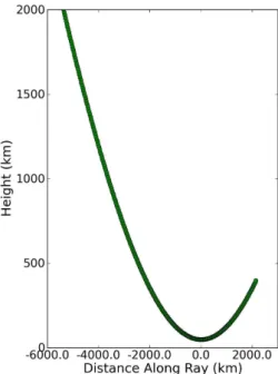
Fig. 1. The altitude of the simulated ray versus distance along the ray, starting at 2000 km altitude. Zero distance is at the ray tangent point. The receiver is on-board CHAMP (400 km altitude orbit).
al., 1991). Variations of electron density near solar maxi-mum daytime conditions must be accounted for to set reli-able upper bounds on the level of ionospheric residual bias in retrievals. Ionospheric storms, which are byproducts of geomagnetic activity, can increase ionospheric residuals sig-nificantly compared to quiet geomagnetic conditions. The residual bias increases for two reasons that often occur si-multaneously during storms: overall electron density values increase as do their spatial gradients. According to propaga-tion physics (Born and Wolf, 1980), the raypaths followed at the L1 and L2 frequencies depend on refractive index magni-tudes and spatial gradients. Separation of raypaths between L1 and L2 generally increases under both density increases and gradient increases for fixed density. Ionospheric storms also undergo “negative” phases, resulting in a significant de-crease of electron density relative to quiet conditions. During these periods, we expect the ionospheric residual to decrease, so we do not explicitly focus on this phase.
In the next section we discuss analysis of the ray-tracing results under representative quiet and disturbed conditions. Our emphasis is on daytime solar maximum conditions when the ionospheric residuals are largest. Simulations for night-time and solar minimum are not considered. We show in detail which parts of the topside and bottomside ionospheric electron density profile are cause for greatest raypath sep-aration, not considering the impact of pronounced E-layers which are important also.
Fig. 2.Electron density versus distance along the simulated raypath. The curves for L1 and L2 frequencies overlay nearly exactly on this scale. The location of the occultation tangent point is shown in the inset.
4 Results
A representative occultation raypath has been selected for de-tailed study in these simulation experiments. The minimum altitude of the raypath (tangent point) is 60 km. At such high altitudes, ionospheric residuals will produce a significant im-pact on retrieval error. The goal of achieving temperature biases less than 0.1 K is unrealistic at 60 km and higher al-titudes, limiting the possibility of using radio occultation in applications where SI-traceability is desired at such high alti-tudes. At lower altitudes, atmospheric bending increases and the impact of ionospheric residuals is less.
We have used the end points of the ray-path from an actual occultation acquired by the CHAMP satellite (Wickert et al., 2001) on 30 October 2003. The altitude of the ray versus dis-tance from the tangent point (ray perigee) is shown in Fig. 1. The location of the raypath tangent point is shown as the in-set in Fig. 2. A severe geomagnetic storm was in progress on 30 October 2003. Very large ionospheric total electron con-tent and electron density spatial gradients were detected by a ground-based GPS receiver network in the vicinity of the occultation ray-path (for details, see Mannucci et al., 2005). This particular occultation geometry was selected to coin-cide with extreme ionospheric conditions as represented by the GAIM.
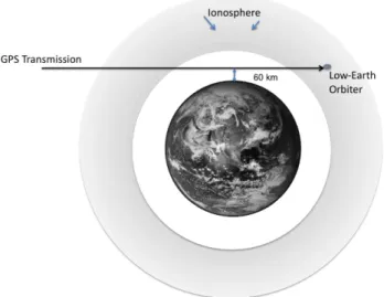
Fig. 3.Schematic representation of the simulated raypath as it en-ters, exits then enters the ionosphere before meeting with the re-ceiver.
conditions. The latter produces much larger gradients than is present in the IRI-95 climatology.
4.1 Results using the International Reference Ionosphere
The IRI-95 model was run for 30 October 2003. The F10.7 solar flux index on that day was 267 (adjusted value), a very high value exceeding by∼48 % the average F10.7 value dur-ing solar maximum years 2000–2001. The electron density encountered along the raypath is shown in Fig. 2. The two-peak structure is a result of twice traversing the ionospheric “annulus”, as shown schematically in Fig. 3. In Fig. 2, the electron densities for the L1 and L2 paths differ impercep-tibly due to the slightly different raypaths and do not ap-pear in this figure. The two electron density peak values oc-cur when the raypath is traversing altitudes 260 and 250 km, near the altitudes of peak electron density in the model (see right panel, Fig. 12, for vertical electron density profiles from the IRI-95 output near the tangent point). Electron densi-ties were linearly extrapolated downward from altitudes of 100 km since the model run cuts off abruptly at that altitude. For this study, we determine the end points of the ray-path from an actual CHAMP orbit when the satellite altitude was 400 km. We will show later that the altitude of the receiver has an impact on the magnitude of the ionospheric residual bias.
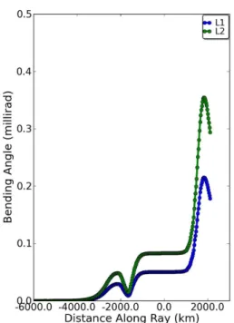
The accumulated bending angle along the raypath for the L1 and L2 frequencies is shown in Fig. 4. The bending an-gle is with respect to the direction that the raypath leaves the transmitter. The angle differs significantly between the two frequencies because of the frequency-dependent refrac-tive index according to the 1/f2 law. The accumulated
Fig. 4. Bending angle along the ray for the L1 and L2 frequencies, assuming IRI electron density distribution extrapolated linearly to zero below 100 km. Bending angle is relative to the direction that the ray leaves the transmitter.
bending angle follows a similar overall pattern for the two frequencies. Several features are notable. Near−1300 km, the accumulated bending angle approaches very low values. At this point along the raypath, the bending due to the top-side ionosphere is nearly compensated for by the oppositely-directed bending in the bottomside, yielding a small net bending value. Shortly after this minimum, the raypath drops below 100 km, effectively exiting the ionosphere. The bend-ing angle increases slowly due to the residual density from the extrapolated IRI profile. The raypath reenters the iono-sphere on the bottom side at ∼1000 km distance, at which
time bending angle increases rapidly again. The electron density peak is reached at∼1900 km distance, at which time
the bending angle direction begins to reverse again. The net bending angle at the receiver is∼0.13 millirad for the L1 frequency, reached at∼2200 km.
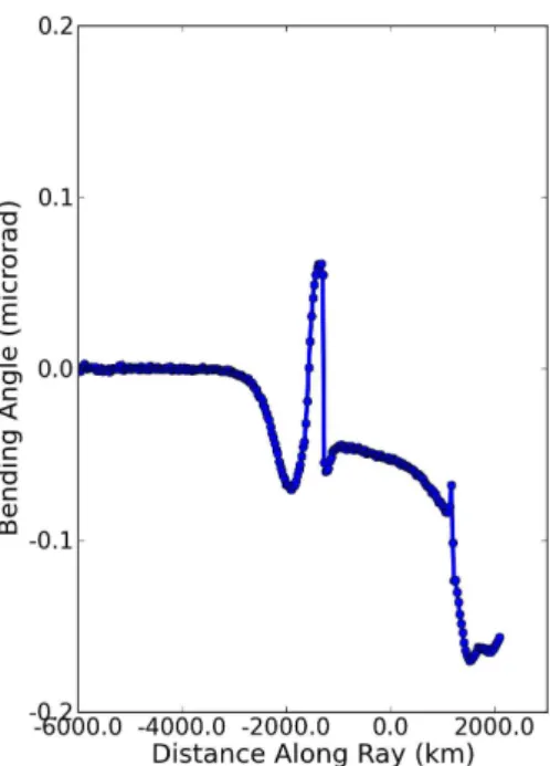
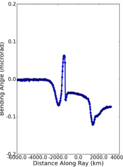
Fig. 5.Residual bending angle after the dual-frequency correction is applied, IRI case.
raypath in Fig. 4. The reduced residual ionosphere at higher altitudes is further discussed in Sect. 4.3.
The linear combination of bending angles at the L1 and L2 frequencies (Eq. 1) produces an estimate of bending caused solely by the neutral atmosphere. Electron density gradients along the L1 and L2 raypaths result in imperfect cancella-tion of ionospheric effects when this formula is applied. In Fig. 5, we plot the residual bending angle calculated from our ray-tracing simulation, assuming the dual-frequency cor-rection is applied. Deviations from zero in Fig. 5 are a mea-sure of ionospheric residual due to raypath separation and higher-order ionospheric effects, either positive or negative depending on whether the dual-frequency correction under-estimates or overunder-estimates the actual bending angle, respec-tively. The residual bending changes rapidly as the raypath enters and exits the first ionospheric traversal. On exiting the ionosphere, the residual bending remains nearly constant with a small bias of∼−3×10⁻⁸ radians. The structure of
the ionosphere results in a fortuitous cancellation of bend-ing angle from the top and bottomsides, as discussed before. Bending angle residual magnitude again begins to increase as the raypath enters the bottomside for the second time (∼1000 km). For this second traversal, cancellation in the topside barely occurs since the satellite is orbiting near the altitude of peak density. At the receiver, the residual bend-ing is∼−6×10⁻⁸ radians, which is the value relevant to retrieval error. If the receiver were at higher altitude, bend-ing cancellation would occur similarly to what occurs in the first ionospheric traversal, reducing the overall impact of the ionosphere on the retrieval. The impact of satellite altitude
Fig. 6. Electron density versus distance along the ray for the sim-ulated raypath assuming the GAIM electron density distribution (compare to Fig. 2).
is discussed later for a low-Earth orbiter (LEO) at COSMIC altitudes (780 km versus 400 km for CHAMP).
4.2 Global assimilative ionosphere model – major ionospheric storm
We use the GAIM to assess the impact of significant elec-tron density gradients that occur during geomagnetic storms, conditions that are not generally captured by the IRI. Plots analogous to those just described for IRI are Figs. 6–8. The transmitter-receiver locations are identical in the two cases. The GAIM assimilates total electron content (TEC) data from the global network of Global Positioning System (GPS) ground receivers and thus captures, at least approximately, horizontal electron gradients and magnitudes that occurred during the storm. The GPS TEC data captures storm condi-tions that occurred on 30 October 2003. The storm is charac-terized by large TEC daytime values, enhanced spatial gra-dients and vertical “uplift” of electron density as reported in Mannucci et al. (2005).
Fig. 7.Bending angle along the ray for the L1 and L2 frequencies, assuming GAIM electron density distribution. Compare to Fig. 4.
Fig. 8.Residual bending angle after the dual-frequency correction (Eq. 1) is applied, GAIM case. Compare to Fig. 5.
Residual bending angle after correction for the storm case is shown in Fig. 8. The residual follows a similar func-tional form for the IRI case. The bending angle affect-ing the retrieval is the value at the receiver location at the ray end-point. This final value is significantly larger in the GAIM case (∼−2.1×10⁻⁷ rad), compared to IRI
(∼−1.5×10⁻⁷ rad). Electron density gradients associated
Fig. 9.Electron density along an occultation ray-path for the storm day, GAIM model case, assuming a spacecraft at COSMIC altitude of 780 km.
with the storm-time redistribution of plasma are a likely con-tributing factor to the increased residual in addition to the overall scalar increase in electron density associated with the storm. Rapid fluctuations in the residual (near−5000 km and 1500 km) are due to numerical noise that arises when spa-tial refractive index derivatives are computed from the GAIM electron density grid.
4.3 Spacecraft orbit considerations
The orbital altitude of the GPS receiver is a significant factor determining the magnitude of the ionospheric residual. The analysis of the previous section shows that ionospheric bend-ing in the topside ionosphere is of opposite sense to bendbend-ing in the bottomside, leading to partial cancellation. The degree of cancellation depends on spacecraft altitude. The analysis just concluded is performed for a spacecraft at the CHAMP altitude of 400 km. We have also computed residual iono-spheric effects for a LEO at 780 km altitude, corresponding to the final altitude of the COSMIC satellites.
Figure 9 shows the electron density along an occultation ray-path for the storm day, IRI case, assuming a spacecraft at COSMIC altitude of 780 km (versus 400 km for CHAMP). The COSMIC raypath tangent point is at approximately the same location as CHAMP (within 1 degree), but the orienta-tion is +233◦
with respect to North. For CHAMP, the orien-tation angle is +137◦
. Orientation angle affects the electron density gradients encountered along the raypath.
The COSMIC altitude is significantly above the altitude of peak electron density (∼400 km). The electron density traces
Fig. 10.Residual bending angle after the dual-frequency correction is applied, GAIM case, for a spacecraft at COSMIC altitude.
both lobes, the electron density is approximately symmetric about the peak. Bending cancellation will be more complete between bottomside and topside. In the comparable CHAMP case (Fig. 2), the electron density at the receiver is close to the peak value at the second lobe. Bending that occurs on the bottomside is not cancelled by bending on the topside. The resulting ionospheric residual bending for the COS-MIC case (780 km altitude) is shown in Fig. 10. The resid-ual bending at the spacecraft location in the COSMIC case (∼−7×10⁻⁸rad) is approximately half the CHAMP value
(∼−1.5×10⁻⁷ rad). More significantly, residual bending
angle in the COSMIC case is clearly reduced by the higher orbit altitude compared to CHAMP. In the CHAMP case, the residual bending angle at the receiver location is 91 % of its peak value (Fig. 2), versus only 60 % of the peak value in the COSMIC case (Fig. 10). If the COSMIC receiver were at CHAMP altitude (2089 km distance along ray), the reduction in residual compared to the peak would be 77 %.
4.4 Retrieval error
The case studies in Sects. 4.1–4.3 illustrate the detailed de-pendence of ionospheric residual on large-scale ionospheric structure and raypath geometry. In this section, we perform an end-to-end simulation to calculate the error in refractivity retrieval due to the ionospheric residual. We perform a full ray-trace calculation through both the ionosphere and atmo-sphere and generate simulated data for use in the retrieval al-gorithm, applying the bending angle correction as described in Eqs. (1) and (2).
The end-to-end simulation system is diagrammed in Fig. 11. Ray-tracing is performed separately for the L1
and L2 signal paths that are propagated to a simulated receiver location at 400 km (CHAMP) or 780 km altitude (COSMIC). As described above, the IRI or GAIM electron density models were used for the ionospheric ray-tracing cal-culation. A spherically-symmetric (radial dependence only) refractivity profile from ECMWF analysis was used for the atmospheric ray-trace calculation, representative of condi-tions on 31 October 2003 near the occultation tangent point at 00:00 UTC (the exact atmospheric profile used is not rel-evant to the analysis). The standard retrieval process is then performed on L1 and L2 phases after perfect subtraction of geometrical distances and assuming perfectly known clocks. After calculation of bending angle at each frequency, the standard ionospheric dual-frequency correction is applied to the bending angles interpolated to common impact parameter (Eq. 1). The retrieved atmospheric refractivity is differenced with the input refractivity. The net result is an estimate of the refractivity residual resulting from imperfectly calibrated ionosphere. We restrict our study to altitudes greater than 20 km, since below that altitude the retrieval bias due to the ionosphere decreases rapidly.
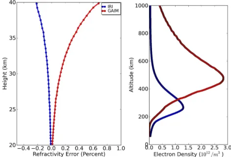
Simulation results are shown in Fig. 12 (left panel), for the GAIM and IRI cases corresponding to 30 October 2003. The raypath geometry is the same as used for the CHAMP case studies. The reason for altitude growth in refractivity bias is that the ionospheric residual remains relatively con-stant with altitude, whereas the atmospheric signal decreases rapidly with altitude. The net result is larger retrieval bias due to the ionospheric residual as altitude increases. Ran-dom error also increases with altitude, an effect which is not included in this simulation.
Fractional refractivity errors between 20–40 km altitudes are significantly larger for the GAIM (storm) case compared to IRI, as expected. The temperature errors resulting from these refractivity biases are not directly available because they depend on additional factors such as the pressure used to initialize the hydrostatic integral. As a general rule, tem-perature errors scale with refractivity error using a factor of
∼200 (e.g. Fig. 9 of Kuo et al., 2004). Thus, the storm time
refractivity biases due to residual ionosphere will produce temperature errors of approximately 0.3 K at 30 km altitude (0.12 % refractivity error), whereas during quiet time tem-perature errors will be closer to 0.1 K. The storm-time er-rors are unacceptably large for climate trend research at al-titudes of 30 km or higher. Kursinski et al. (1997) reported 0.12 % refractivity error due to residual ionosphere at 30 km altitude for quiet-time solar maximum daytime conditions, versus 0.05 % we find using IRI. Kursinski et al. (1997) used one-dimensional raytracing through a Chapman layer rather than the higher-fidelity IRI electron density model. These different results may be consistent with the fact that different ionospheric electron density models are used and the sensi-tivity to electron density vertical gradients.
Fig. 11.Processing chain for the end-to-end simulation.
major error source that affects retrieval accuracy at high al-titude is initialization of the Abel transform used to compute refractivity from bending angle (Hajj et al., 2002). The upper limit for the Abel transform is formally infinite. Often, an ap-proximate functional form for the bending angle vertical pro-file is used (e.g. exponential decay) to extend the integral in altitude. Alternatively, climatological models of the neutral atmosphere might be used to compute bending angles at high altitudes. Both of these methods of extending the Abel trans-form beyond the altitude of the highest bending angle mea-surement introduce error in the retrieved refractivity profile. To avoid retrieval error due to extrapolation, the following procedure is followed here. The retrieved refractivity pro-file is based on bending angle propro-files derived from the ray-trace calculation through the appropriate ionosphere (GAIM or IRI). This computation of refractivity requires the Abel transform, which we truncate at 70 km altitude rather than “infinity”. This truncation introduces some error in the re-trieval that is not due to ionosphere. To compensate, the “truth” refractivity we use contains the same truncation er-ror, so that truncation error does not contribute to the dif-ferences shown in Fig. 12. The modified truth refractivity is derived, via Abel, from a “truth” bending angle profile. The truth bending angle profile is then truncated (set to zero) above 70 km altitude prior to the Abel being applied. (This truncation is similar to what is performed for bending an-gles from the raytrace simulation). The modified truth bend-ing angle is computed exactly from the input truth refrac-tivity (ECMWF) via the inverse Abel transform extended to 100 km altitude. Therefore, truncating the truth bending an-gle at 70 km and then applying the Abel transform guarantees that the modified truth refractivity and the refractivity from raytracing contain the same Abel truncation errors.
It is useful to consider the impact of electron den-sity variation on the retrieval accuracy. The right panel of Fig. 12 shows the electron density profiles near the occultation tangent point (33◦N, 97◦W) for the GAIM and IRI cases. Storms are not the only cause of electron density variation in the ionosphere. Variable solar insolation (X-ray and extreme ultraviolet wavelengths) and local “ionospheric weather” factors modulate electron densities during nominal conditions also. Such modulation can reach factors of two even for a common local time (Brown et al., 1991). Natural ionospheric variability and its representation in simulations may be affecting the results of different simulations appear-ing in the literature (e.g. Kursinski et al., 1997; Steiner et al., 2001). Refractivity bias due to ionospheric residual will generally increase with increasing electron density, of which storms can provide an extreme case (right panel, Fig. 12).
Fig. 12. Left panel: retrieval simulation results plotted as refractivity fractional error, for the IRI and GAIM cases. CHAMP satellite geometry is assumed. Right panel: vertical electron density profiles near the occultation tangent point.
Fig. 13.Left panel: refractivity error assuming unity refractive index at the receiver, versus using the actual refractivity given by the GAIM electron density estimate, for the CHAMP raypath geometry. Right panel: same as the left panel but for the COSMIC raypath geometry.
Retrieval error is also affected by an assumption made that the refractive indices at the receiver and transmitter are both unity (Hajj et al., 2002). While unity holds at the transmit-ter, refractive index is not unity at the receiver, particularly when the receiver is near the peak ionospheric electron den-sity, as is the case for CHAMP. Figure 13 shows the con-tribution to retrieval error from the assumption that refrac-tive index is unity at the receiver, for the GAIM case. (The contribution to retrieval error from truncation of the Abel is
reduce the impact of ionospheric residual need to account for refractive index at the receiver, at least for receivers near the topside ionosphere.
5 Discussion
This analysis shows that details of the electron density distri-bution and orbit altitude are two major factors in determining biases that occur due to ionospheric residual, affecting upper troposphere and lower stratosphere atmospheric retrievals. Ionospheric residual is sensitive to spacecraft altitude since the vertical distribution of ionospheric electron density can reach a peak near orbital altitudes of low Earth orbiting re-ceivers. Residual error accumulated as rays traverse the bot-tom side ionosphere below the peak density tend to cancel residual error of opposite sign as the ray traverses the topside above the peak. For spacecraft near the peak electron den-sity altitude, such as CHAMP (∼400 km), there is minimal topside/bottomside cancellation. Satellites orbiting near the peak of electron density are also more susceptible to the error made by ignoring refractive index at the receiver.
We have for the first time used an ionospheric data assimi-lation model to assess ionospheric residual during storm ditions. As expected, residuals increase significantly for con-ditions characteristic of the major disturbance known as the “Halloween Storms” of 29–30 October 2003. For long-term climate applications of GPS data, it is important to remove such active periods from climatological averages. The num-ber of such excised days is likely to be insignificant if only the most extreme events are considered, which typically per-sist 1–2 days and occur perhaps 5–10 times per 11-yr solar cycle. Further research is needed to understand how the full spectrum of ionospheric disturbances can affect the residual error during the declining phase of the solar cycle, since it is likely that moderately disturbed conditions have an impact also. We note that recent solar-terrestrial research shows that during the declining phase of the solar cycle moderately ac-tive conditions can persist for days to weeks. These long-duration, mild geomagnetic conditions are due to the pres-ence of coronal holes, which migrate to lower latitudes on the solar surface during the declining phase (Tsurutani et al., 2006).
This study generally agrees with past efforts in charac-terizing the magnitude of the ionospheric residual on re-trieval error. However, there is a spread in past research likely due to the detailed assumptions used regarding iono-spheric structure, the magnitudes of electron density consid-ered, and whether E-region layers are included. We believe that even at 20 km altitude, ionospheric residual remains too large for climate monitoring applications during daytime so-lar maximum conditions. Although past studies may cor-rectly conclude that RO is ready for observing long-term cli-mate (Steiner et al., 2001; Steiner et al., 2009), we believe “the margin for error” is too narrow and should be safer.
Continuing efforts are encouraged to develop algorithms that reduce the ionospheric residual error using improved al-gorithms and techniques (Ladreiter and Kirchengast, 1996; Gorbunov et al., 1996; Syndergaard, 2000). As discussed by Gorbunov et al. (1996) the bending angle correction for-mula (Eq. 1) implicitly relies on a linear relationship between bending angle and phase delay due to the ionosphere. Such linearity is violated by raypath separation and non-spherical symmetry of large-scale ionospheric structure. Clearly there are opportunities for robust correction algorithms that im-prove upon Eq. (1).
We emphasize that this study is restricted to ionospheric residuals due to large-scale structure. Recent work (Zeng and Sokolovskiy, 2010) has emphasized the impact of small-scale structure in the E-region (∼120 km altitude). Such structures are not part of the current study since neither the IRI nor GAIM models reproduce them effectively. Fortunately, for climate applications the presence of these structures gener-ally produces distinct fluctuations in the data, so that miti-gating approaches can be devised. Further work is needed to characterize the frequency and distribution of such structures in the context of global climate monitoring. We note also that at high altitudes, initialization of the Abel integral may also introduce significant errors in the retrieval (Hajj et al., 2002). These errors are likely to have a different impact than ionosphere on climatological averages formed from RO data. It is likely that long-term climate records will combine a mix of RO satellites orbiting at varying altitudes. Our analysis shows a significant impact of orbit altitude on the magnitude of ionospheric residual bending. Therefore, care must be exercised when creating the long-term record, to avoid small systematic biases that might vary with mission. Clearly, this matter is tied to the overall question of reduc-ing ionospheric residuals to achieve greater margin for error in forming climate averages from RO data. As part of this margin, we recommend that ionospheric activity indices be consulted to make sure that increased ionospheric activity is not affecting the record.
6 Conclusions
We have performed a detailed propagation study for GPS signals in an occulting geometry to gain insight into the sources of residual ionospheric bias affecting upper tropo-sphere/lower stratospheric retrievals. This is the first study to address the case of severe geomagnetic storms that cre-ate large electron density magnitudes and spatial gradients in the ionosphere. The large resulting retrieval bias suggests that monitoring ionospheric conditions is a necessary prereq-uisite for long-term climate observation with RO, to excise those periods from the record where the level of ionospheric disturbance is unacceptably high.
easily exceed 25 % or more, depending on details of the orbit altitude and altitude of peak ionospheric refraction index). Care must be exercised to account for possible bias differ-ences when forming long-term climate averages using multi-ple satellite time series of data.
The way forward for climate monitoring applications is to develop a strategy for setting robust upper bounds to iono-spheric residual bias under a wide variety of solar and ge-omagnetic conditions. This upper bound is the means by which RO retrievals can maintain SI-traceability in the pres-ence of ionospheric effects. Given the size of the bias above 25 km, it is highly desirable to develop ionospheric correc-tion algorithms that are more accurate and robust than the standard dual-frequency bending angle correction. Even with improved algorithms, there will be disturbances for which the residual bias is unacceptably large and in such cases the RO retrievals should not be included in long-term climate av-erages. This implies that some form of space weather moni-toring should be implemented as part of the climate observa-tion strategy, to ensure that disturbed condiobserva-tions do not play a disproportionately large role in the climate averages.
Acknowledgements. The research for this paper was performed at the Jet Propulsion Laboratory, California Institute of Technology under contract with NASA. The authors wish to acknowledge support of the NASA Earth Science Directorate.
Edited by: U. Foelsche
References
Bassiri, B. and Hajj, G.: Higher-order ionospheric effects on the global positioning system observables and means of modeling them, Manuscripta Geodaetica, 18, 280–289, 1993.
Bilitza, D. and Reinisch, B. W.: International Reference Ionosphere 2007: Improvements and new parameters, Adv. Space Res., 42, 599–609, doi:10.1016/j.asr.2007.07.048, 2008.
Born, M. and Wolf, E.: Principles of Optics: Electromagnetic The-ory of Propagation, Interference and Diffraction of Light, 6th Edition, Pergamon, Elmsford, NY, 1980.
Brown, L. D., Daniell, R. E., Fox, M. W., Klobuchar, J. A., and Doherty, P. H.: Evaluation of 6 ionospheric models as predictors of total electron-content, Radio Science, 26, 1007–1015, 1991. Budden, K. G.: The Propagation of Radio Waves, Cambridge
Uni-versity Press, New York, NY, 1985.
Davies, K.: Ionospheric Radio, The Institution of Engineering and Technology, London, 1990.
Fox, N., Kaiser-Weiss, A., Schmutz, W., Thome, K., Young, D., Wielicki, B., Winkler, R., and Woolliams, E.: Accurate ra-diometry from space: an essential tool for climate studies, Phi-los. Trans. R. Soc. A-Math. Phys. Eng. Sci., 369, 4028–4063, doi:10.1098/rsta.2011.0246, 2011.
Goody, R., Anderson, J., and North, G.: Testing climate models: An approach, B. Am. Meteorol. Soc., 79, 2541–2549, 1998. Gorbunov, M. E., Sokolovsky, S. V., and Bengtsson. L.: Space
re-fractive tomography of the atmosphere: Modeling of direct and
inverse problems, Rep. Max Planck Inst for Meteorol., No. 210-59, Hamburg, Germany, 1996.
Hajj, G. A., Kursinski, E., R., Romans, L. J., Bertiger, W. I., and Leroy, S. S.: A technical description of atmospheric sounding by GPS occultation, J. Atmos. Solar-Terr. Phys., 64, 451–469, 2002. Hajj, G. A., Ao, C. O., Iijima, B. A., Kuang, D., Kursinski, E. R., Mannucci, A. J., Meehan, T. K., Romans, L. J., de la Torre Juarez, M., and Yunck, T. P.: CHAMP and SAC-C atmospheric occultation results and intercomparisons, J. Geophys. Res., 109, D06109, doi:10.1029/2003JD003909, 2004.
Hayashi, H., Furumoto, J. I., Lin, X. N., Tsuda, T., Shoji, Y., Aoyama, Y. and Murayama, Y.: Validation of Refractivity Pro-files Retrieved from FORMOSAT-3/COSMIC Radio Occultation Soundings: Preliminary Results of Statistical Comparisons Uti-lizing Balloon-Borne Observations, Terrestrial Atmos. Ocean. Sci., 20, 51–58, doi:10.3319/tao.2008.01.21.01(f3c), 2009. He, W. Y., Ho, S. P., Chen, H. B., Zhou, X. J., Hunt, D., and Kuo,
Y. H.: Assessment of radiosonde temperature measurements in the upper troposphere and lower stratosphere using COS-MIC radio occultation data, Geophys. Res. Lett., 36, L17807, doi:10.1029/2009gl038712, 2009.
Hoque, M. M., and Jakowski, N.: Higher order ionospheric propa-gation effects on GPS radio occultation signals, Adv. Space Res., 46, 162–173, doi:10.1016/j.asr.2010.02.013, 2010.
International Association of Geomagnetism and Aeronomy (IAGA), D. V., Working Group 8: The 9th Generation Interna-tional Geomagnetic Reference Field, Earth Planet. Space, 55, i-ii, 2003.
Kuo, Y. H., Wee, T. K., Sokolovskiy, S., Rocken, C., Schreiner, W., Hunt, D., and Anthes, R. A.: Inversion and error estimation of GPS radio occultation data, J. Meteorol. Soc. Jpn., 82, 507–531, 2004.
Kuo, Y. H., Schreiner, W. S., Wang, J., Rossiter, D. L., and Zhang, Y.: Comparison of GPS radio occultation sound-ings with radiosondes, Geophys. Res. Lett., 32, L05817, doi:10.1029/2004gl021443, 2005.
Kursinski, E. R., Hajj, G. A., Bertiger, W. I., Leroy, S. S., Mee-han, T. K., Romans, L. J., Schofield, J. T., McCleese, D. J., Mel-bourne, W. G., Thornton, C. L., Yunck, T. P., Eyre, J. R., and Nagatani, R. N.: Initial results of radio occultation observations of Earth’s atmosphere using the global positioning system, Sci-ence, 271, 1107–1110, 1996.
Kursinski, E. R., Hajj, G. A., Schofield, J. T., Linfield, R. P., and Hardy, K. R.: Observing Earth’s atmosphere with radio occulta-tion measurements using the Global Posiocculta-tioning System, J. Geo-phys. Res.-Atmos., 102, 23429–23465, 1997.
Ladreiter, H. P. and Kirchengast, G.: GPS/GLONASS sensing of the neutral atmosphere: Model-independent correction of iono-spheric influences, Radio Science, 31, 877–891, 1996.
Mannucci, A. J., Wilson, B. D., Yuan, D. N., Ho, C. H., Lindqwis-ter, U. J., and Runge. T. F.: A global mapping technique for GPS-derived ionospheric total electron content measurements, Radio Science, 33, 565–582, 1998.
G. A., Iijima, B. A., Kuang, D., Meehan, T. K., and Leroy, S. S.: Generating climate benchmark atmospheric soundings using GPS occultation data, SPIE Proceedings, 6301, 630108, doi:10.1117/12.683973, 2006.
Ohring, G., Wielicki, B., Spencer, R., Emery, B., and Datla, R.: Satellite instrument calibration for measuring global climate change – Report of a Workshop, B. Am. Meteorol. Soc., 86, 1303–1313, 2005.
Rocken, C., Anthes R., Exner M., Hunt, D., Sokolovskiy, S., Ware, R., Gorbunov, M., Schreiner, W., Feng, D., Herman, B., Kuo, Y. H., and Zou, X.: Analysis and validation of GPS/MET data in the neutral atmosphere, J. Geophys. Res.-Atmos., 102, 29849– 29866, 1997.
Schreiner, W., Rocken, C., Sokolovskiy, S., Syndergaard, S., and Hunt, D.: Estimates of the precision of GPS radio occultations from the COSMIC/FORMOSAT-3 mission, Geophys. Res. Lett., 34, L04808, doi:10.1029/2006gl027557, 2007.
Sokolovskiy, S., Schreiner, W., Rocken, C., and Hunt, D.: Opti-mal Noise Filtering for the Ionospheric Correction of GPS Radio Occultation Signals, J. Atmos. Ocean. Technol., 26, 1398–1403, doi:10.1175/2009jtecha1192.1, 2009.
Steiner, A. K. and Kirchengast, G.: Error analysis for GNSS ra-dio occultation data based on ensembles of profiles from end-to-end simulations, J. Geophys. Res.-Atmos., 110, D15307, doi:10.1029/2004JD005251, 2005.
Steiner, A. K., Kirchengast, G., and Ladreiter, H. P.: Inversion, er-ror analysis, and validation of GPS/MET occultation data, Ann. Geophys.-Atmos. Hydrospheres Space Sci., 17, 122–138, 1999. Steiner, A. K., Kirchengast, G., Foelsche, U., Kornblueh, L.,
Manzini, E., and Bengtsson, L.: GNSS occultation sounding for climate monitoring, Phys. Chem. Earth Pt. A-Solid Earth Geod., 26, 113–124, 2001.
Steiner, A. K., Kirchengast, G., Lackner, B. C., Pirscher, B., Borsche, M., and Foelsche, U.: Atmospheric temperature change detection with GPS radio occultation 1995 to 2008, Geophys. Res. Lett., 36, L18702, doi:10.1029/2009gl039777, 2009.
Sun, B. M., Reale, A., Seidel, D. J., and Hunt, D. C.: Compar-ing radiosonde and COSMIC atmospheric profile data to quantify differences among radiosonde types and the effects of imperfect collocation on comparison statistics, J. Geophys. Res.-Atmos., 115, D23104, doi:10.1029/2010jd014457, 2010.
Syndergaard, S.: On the ionosphere calibration in GPS radio occul-tation measurements, Radio Science, 35, 865–883, 2000. Tsurutani, B. T., Gonzalez, W. D., Gonzalez, A. L. C., Guarnieri,
F. L., Gopalswamy, N., Grande, M., Kamide, Y., Kasahara Y., Lu, G., Mann I., McPherron, R., Soraas F., and Vasyliunas, V.: Corotating solar wind streams and recurrent geomagnetic ac-tivity: A review, J. Geophys. Res-Space Phys., 111, A07S01, doi:10.1029/2005JA011273, 2006.
Vergados, P. and Pagiatakis, S. D.: First estimates of the second-order ionospheric effect on radio occultation ob-servations, J. Geophys. Res-Space Phys., 115, A07317, doi:10.1029/2009ja015161, 2010.
Vorobev, V. V. and Krasilnikova, T. G.: An estimation of accuracy of the atmospheric refractive-index recovery from measurements of doppler shifts at frequencies used in the navstar system, Izvestiya Akademii Nauk Fizika Atmosfery I Okeana, 29, 602–609, 1993. Wang, C. M., Hajj, G., Pi, X. Q., Rosen, I. G., and Wilson, B.: De-velopment of the Global Assimilative Ionospheric Model, Radio Science, 39(1), RS1S06, doi:10.1029/2002rs002854, 2004. Wickert, J., Reigber, C., Beyerle, G., K¨onig, R., Marquardt, C.,
Schmidt, T., Grunwaldt, L., Galas, R., Meehan, T. K., Mel-bourne, W. G., and Hocke, K.: Atmosphere sounding by GPS ra-dio occultation: First results from CHAMP, Geophys. Res. Lett., 28, 3263–3266, doi:10.1029/2001gl013117, 2001.
Xu, X. H., Luo, J., and Shi, C. A.: Comparison of COSMIC Ra-dio Occultation Refractivity Profiles with RaRa-diosonde Measure-ments, Adv. Atmos. Sci., 26, 1137–1145, doi:10.1007/s00376-009-8066-y, 2009.