www.nonlin-processes-geophys.net/21/617/2014/ doi:10.5194/npg-21-617-2014
© Author(s) 2014. CC Attribution 3.0 License.
Distinguishing the effects of internal and forced atmospheric
variability in climate networks
J. I. Deza1, C. Masoller1, and M. Barreiro2
1Departament de Física i Enginyeria Nuclear, Universitat Politècnica de Catalunya, Colom 11, 08222, Terrassa, Barcelona, Spain
2Instituto de Física, Facultad de Ciencias, Universidad de la República, Iguà 4225, Montevideo, Uruguay
Correspondence to:J. I. Deza ([email protected])
Received: 31 October 2013 – Revised: 3 March 2014 – Accepted: 20 March 2014 – Published: 26 May 2014
Abstract. The fact that the climate on the earth is a highly complex dynamical system is well-known. In the last few decades great deal of effort has been focused on understand-ing how climate phenomena in one geographical region af-fects the climate of other regions. Complex networks are a powerful framework for identifying climate interdependen-cies. To further exploit the knowledge of the links uncov-ered via the network analysis (for, e.g., improvements in pre-diction), a good understanding of the physical mechanisms underlying these links is required. Here we focus on under-standing the role of atmospheric variability, and construct climate networks representing internal and forced variabi-lity using the output of an ensemble of AGCM runs. A main strength of our work is that we construct the networks us-ing MIOP (mutual information computed from ordinal pat-terns), which allows the separation of intraseasonal, intra-annual and interintra-annual timescales. This gives further insight to the analysis of climatological data. The connectivity of these networks allows us to assess the influence of two main indices, NINO3.4 – one of the indices used to describe ENSO (El Niño–Southern oscillation) – and of the North Atlantic Oscillation (NAO), by calculating the networks from time se-ries where these indices were linearly removed. A main result of our analysis is that the connectivity of the forced variabi-lity network is heavily affected by “El Niño”: removing the NINO3.4 index yields a general loss of connectivity; even teleconnections between regions far away from the equato-rial Pacific Ocean are lost, suggesting that these regions are not directly linked, but rather, are indirectly interconnected via El Niño, particularly at interannual timescales. On the contrary, on the internal variability network – independent of sea surface temperature (SST) forcing – the links
connect-ing the Labrador Sea with the rest of the world are found to be significantly affected by NAO, with a maximum at intra-annual timescales. While the strongest non-local links found are those forced by the ocean, the presence of teleconnections due to internal atmospheric variability is also shown.
1 Introduction
The existence of long-range teleconnections in climate is an established fact, as the atmosphere connects far-away regions through waves and advection of heat and momentum. This long-range coupling makes the complex network approach (Albert and Barabási, 2002) of the earth’s climate very attrac-tive (Tsonis et al., 2006, 2008; Donges et al., 2009b). Climate networks are constructed by considering the earth as a regu-lar grid of nodes and assigning links connecting two different nodes via an analysis of their similarity over a particular field. This approach has been used in the literature both on local and on global scales and for analyzing climate phenomena considering both linear and nonlinear interdependencies.
For example, the network approach has been recently used to analyze patterns of extreme monsoonal rainfall over South Asia (Malik et al., 2012), to infer early warning indicators for the Atlantic Meridional Overturning Circulation collapse (van der Mheen et al., 2013), to gain insight into the origin of decadal climate variability (Tsonis and Swanson, 2012) and to study the El Niño phenomenon as an autonomous compo-nent of the climate network (Gozolchiani et al., 2011).
etc.) and the reliability and robustness of the networks un-covered have also been analyzed in terms of a critical com-parison of the networks found with the various methods used (Paluš et al., 2011; Hlinka et al., 2013; Martin et al., 2013; Tirabassi and Masoller, 2013). A main conclusion of these studies is that it is crucial to analyze the robustness of the method used to quantify climate similarities because trends and serial correlations in the time series, as well as time lags, can significantly affect the topology of the network obtained. This paper is focused on understanding the atmospheric variability by means of networks constructed from monthly averaged surface air temperature (SAT) anomalies.
Atmospheric variability can be considered, to first order, as a superposition of an internal part due to intrinsic dynam-ics, and an external part due to the variations of the boundary conditions, primarily given by the sea surface temperature (SST) forcing. These two components can be distinguished by using atmospheric general circulation models (AGCMs) forced with prescribed historical SSTs (Straus and Shukla, 2000; Barreiro et al., 2002; Molteni, 2003; Bracco et al., 2004) – see also the accompanying paper (Arizmendi et al., 2014) in this Special Issue.
The separation between internal and forced atmospheric variability is a standard procedure to study the impact of the oceans on the atmosphere and has led to important advances regarding our understanding of the dynamics involved. James (1995) and Trenberth (1997) provide two excellent sum-maries of the processes involved, mainly based on the propa-gation of Rossby waves and the generation of teleconnection patterns. Although there are some nonlinear secondary ef-fects, the theory asserts that, to first order, the observed prop-agation and establishment of teleconnection patterns are lin-ear.
Separating forced from internal atmospheric variability is also important because it can allow for improvements in climate prediction. In many geographical regions, the atmosphere is strongly influenced by SST variations that force persistent anomalies (Shukla, 1998). Because the evo-lution of the tropical oceans presents some predictability at timescales longer than the atmosphere, prediction of atmo-spheric variables beyond the chaotic timescale of 7–10 days is possible, provided that the atmospheric dynamics have been forced by the ocean (Shukla, 1998).
The usual modeling strategy to study predictability con-sists in forcing AGCMs with idealized or observed SST anomalies. This allows for investigating the response of the atmosphere to different boundary conditions and different initial conditions. If the time series of anomalies of a cli-matic field (e.g., SAT anomalies) is considered as a combi-nation of internal and forced variability (e.g.,x=xfor+xint) the output of several numerical experiments initialized dif-ferently but forced with thesameboundary conditions (i.e., same SST) can be used to separate the internal and forced
variability. For each runiit results in xi=xfori +xinti =xfor+xinti
(asxfordoes not depend on the initial conditions). Averaging overNruns yields
¯
x=xfor+(1/N ) X
i
xinti .
IfN is large enough, the second term will be small, as each model run will have a different value. Thus, to the first order
¯
x≈xfor.
In other words, each time seriesxi can be separated into a part that changes from run to run,xinti , and a part that does not depend on the initial conditions (is forced by the boundary conditions only and is the same for all runs),xfor≈ ¯x.
This method allows for the construction of two types of networks, those in which the links represent similarities in in-ternal atmospheric variability (referred to asinternal variabi-litynetwork), and those in which the links represent similar-ities in forced atmospheric variability (theforced variability network).
The connectivity of these networks allows us to assess the influence of two main phenomena: El Niño (characterized by the NINO3.4 index) and the North Atlantic Oscillation (cha-racterized by the NAO index). This was done by calculating the networks from time series where either the NINO3.4 in-dex or the NAO inin-dex was linearly removed.
The forced variability networks is found to be intimately related to El Niño phenomenon and that linearly removing its evolution yields a breakdown of the long-range telecon-nections of the climate network, particularly at interannual timescales. A similar result is observed for the internal varia-bility network in the Northern Hemisphere when NAO is re-moved, with the maximum effect at intra-annual timescales.
The paper is organized as follows. In Sect. 2 the method used for constructing climate networks is shown. The data and the model, employed as well as the NINO3.4 and NAO indices, are discussed in Sect. 3. Section 4 presents the re-sults. Here the internal and forced variability networks, and the effects of NAO and El Niño are analyzed. Section 5 presents a summary and the conclusions.
2 Methods for network construction 2.1 Measure of statistical interdependence
The mutual information (MI) is computed from the proba-bility density functions (PDFs) that characterize two time se-ries in two nodes,piandpj, as well as their joint probability
function,pij(Cover and Thomas, 2006; Amigó, 2010; Paluš,
2007):
Mij= X
m,n
pij(m, n)log
pij(m, n)
pi(m)pj(n)
Mij is a symmetric measure (Mij =Mj i) of the degree of
statistical interdependence of the time series in nodesiand j; if they are independentpij(m, n)=pi(m)pj(n), and thus
Mij=0.
In this paper the PDFspi,pj, andpijare computed in two
ways: by histograms of values (this case will be referred to as MIH) and by using a symbolic transformation, in terms of probabilities ofordinal patterns(this case will be referred to as MIOP) (Amigó, 2010; Pompe and Runge, 2011; Bandt and Pompe, 2002; Barreiro et al., 2011).
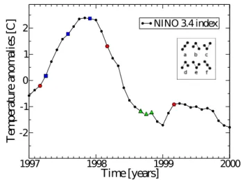
The ordinal patterns are calculated from time series by comparing the value of a given data point relative to its neigh-bors (Fig. 1). When a value (v2) is higher than the previous one (v1) and lower than the next one (v3) (v1< v2< v3), the ordinal transformation gives pattern “a” (see inset in Fig. 1); when v1> v2> v3, it gives pattern “f”, and so forth. Con-sidering patterns of lengthD, then there areD!possible pat-terns.
A significant advantage of MIOP for climate data analysis over other methods is that the ordinal transformation allows us to select the timescale of the analysis, not only by con-sidering shorter or longer patterns, but also, by comparing data points in the time series which are not consecutive, but separated by a time interval.
This symbolic transformation keeps the information about correlations present in a time series at the selected timescale, but does not keep information about the absolute values of the data points. Therefore, the mutual information com-puted from ordinal patterns (MIOP) can be expected to pro-vide complementary information with respect to the standard method of computing the mutual information (MIH) with monthly averaged data and zero-lag regressions, adequate for many geographical regions of earth. However, there are some exceptions, and the analysis of lagged responses could be an interesting extension of the present study that is left for future work.
Monthly data in the period January 1948–December 2006 is analyzed. Due to the short length of the time series (708 data points), in order to compute the probabilities of the patterns with good statistics we have considered ordinal pat-terns of length three. Since forD=3 there are six possible
patterns, for the sake of consistency, the MIH is computed using histograms with 6 equi-sized bins.
We varied the timescale of the MIOP analysis by con-structing the patterns in three ways (see Fig. 1): (1) by com-paring temperature anomalies in 3 consecutive months (constructing patterns with three consecutive data points), (2) by comparing anomalies in 3 equally spaced months that cover a 1-year period (by taking one data point every four points), and (3) by comparing anomalies in the same month of 3 consecutive years (by taking one data point every twelve points). The MIOP computed in these ways is referred to asintraseasonal,intra-annual, andinterannual, respectively. While constructing the patterns with one data point per sea-son (i.e., every three points) could seem more useful – as
1997 1998 1999 2000
Time[years] -2 -1 0 1 2 T em pe ra tu re an om al ie s [C
] NINO 3.4index
Figure 1.An example of three ordinal patterns in the time series of
the NINO3.4 index (monthly averaged). Green triangles: intrasea-sonal pattern, blue squares: intra-annual pattern and red circles: in-terannual pattern. The possible patterns forD=3 are shown in the inset. In this example, the intraseasonal pattern corresponds to an “e”, the intra-annual, to an “a” and the interannual, to a “b”.
seasons cover 3 months– we decided to use 3 data points per year because seasons are not well-defined worldwide (for ex-ample, in the tropics), but the seasonal cycle is.
2.2 Definition of links
To construct the network, a link between nodesiandj is de-fined ifMij is above an appropriate threshold, which is
cal-culated in terms ofsurrogate-shuffled data as in Deza et al. (2013), where the data are shuffled before we calculate the histograms or the ordinal patterns. When defining the sig-nificance criterion for the links in climate networks there is always a degree of arbitrariness. As we have shown in our previous work, the distribution of MI values computed from surrogate data is approximately Gaussian (see Fig. 1 of Deza et al., 2013). Therefore, here we use a significance criterion computed in terms of the mean,µ, and the standard devia-tion,σ, of the distribution of MI values computed from sur-rogate data, and accept links whose MI value, computed from the original data, is aboveµ+3σ.
While this is the simplest approach, it has well-known drawbacks (see, e.g., Schreiber and Schmitz, 1996; Paluš, 2007), and the use of block surrogates and/or quantile thresh-olds, as significance criterion will provide a valuable and computationally not too demanding improvement to the method used here.
2.3 Network representation
area of earth to which each node is connected, that is,
AWCi= PN
j Aijcos λj PN
j cos λj
,
whereλi is the latitude of nodeiandAij=1 if nodesiand
j are connected, and 0 otherwise (Tsonis et al., 2008). It is of particular interest to identify significant weak links, as the strongest links are usually of shorter spatial range. In all the AWC maps presented in Sect. 4, the color scale has been set from 0 to a fixed value (0.4), and any node with stronger connectivity is shown with the color code of 0.4. This allows a clearer visualization the weakest part of the accepted sig-nificant links. It also allows for a direct comparison of all the AWC maps.
In Sect. 4 the significant connections of some selected geo-graphical regions (represented by individual network nodes) are explored. In these connectivity maps the value of the in-terdependency measure (MIH or MIOP) will be displayed using a color scale which is also fixed, from 0 up to 0.3; MI values larger than this will be shown using the same color code as 0.3.
3 Data sets and model used 3.1 Climate indices
A climate index describes the state and changes of a par-ticular region of the ocean or the atmosphere. Indices can be determined from monitoring station or reanalysis data, or identified by means of empirical orthogonal functions (EOF) analysis. In the latter case, they result in the principal com-ponent (PC) related to an EOF (generally the leading mode) over a chosen area, calculated for a predetermined variable (e.g., temperature or pressure). As explained below, the av-erage of SST on the NINO3.4 area has been used for calcu-lating the NINO3.4 index, and the leading PC over the North Atlantic region has been used to calculate NAO. The indices have been linearly detrended.
3.1.1 NINO 3.4
The NINO3.4 index (Trenberth, 1997) was calculated as the average of SST anomalies in the equatorial Pacific bounded by latitudes 5◦S–5◦N and by longitudes 120◦W–170◦W, using the SST data incorporated by the model as a bound-ary condition for all the runs. The index, obtained in this way, has been compared with the monthly index from NOAA (2013), updated monthly, obtaining an excellent agreement. As this index is based on SST – a boundary condition for the AGCM – this phenomenon can be expected to affect mainly theforcedpart of the atmospheric variability.
3.1.2 NAO
The North Atlantic Oscillation (NAO) has been shown to be mainly anatmosphericphenomenon only weakly forced by the ocean (Hurrel, 1995). The NAO index is calculated as the leading EOF of surface pressure over the North At-lantic region (20◦–80◦N and 90◦W–40◦E) for each model run. Comparison among indices from different model runs and between these and the observed NAO index from NCEP/NCAR reanalysis data yielded different time series modulating essentially the same spatial pattern. The NAO properties have been studied elsewhere (see Lind et al., 2005, and references therein), but for our purposes it is enough to assume that these series have the same power spectra as low frequency noise.
3.2 Model used
In this study the AGCM from the International Centre for Theoretical Physics (ICTP AGCM) has been used. It con-sists of a full atmospheric model with simplified physics and a horizontal resolution of T30 (3.75◦×3.75◦, which gives
N=608 grid points or network nodes) with eight vertical
levels (Molteni, 2003). The model is forced with histori-cal global sea surface temperatures (ERSSTv.2) (Smith and Reynolds, 2004). In order to separate forced from internal atmospheric variability, nine runs using the same boundary (SSTs) conditions (but slightly different initial conditions) were performed.
contamination are discussed in Allen and Smith (1997), Ven-zke et al. (1999), Barreiro et al. (2002, 2005), and Ting et al.
(2009).
Monthly averaged air surface temperature (SAT) in the pe-riod January 1948–December 2006 was analyzed. This re-sults in a total of 708 data points per node. For each node, the time series were linearly detrended and the anomalies of these series were computed by subtracting the long term av-erage to each monthly data point.
The influence of NINO3,4 or NAO indices was assessed by computing time series where one of these indices was linearly removed from the original time series, respectively. This was done in three steps:
1. calculate the indices, as explained above;
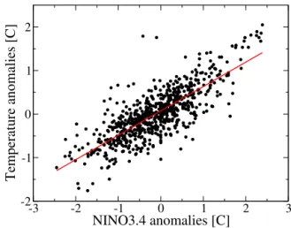
2. perform a zero-lag regression of the time series of each node with respect to the time series of the index (see Fig. 2);
3. subtract the linear regression from the original data. In the following section it is shown that this procedure ef-fectively removes the linear contribution of the given index in the evolution of each node (Rodwell et al., 1999; Barreiro, 2009). However, this simple approach for assessing the influ-ence of an index could be improved in two ways: on the one hand, nonlinear methods for calculating the index could be considered (see e.g., Gámez et al., 2004), on the other hand, lagged regressions could be considered.
To validate the model (see Sect. 4.1) we considered re-analysis data from NCEP/NCAR (Kalnay, et al., 1996) in the same time period (1948–2006). Since NCEP/NCAR reanaly-sis data are given on a 2.5◦×2.5◦grid, for easier comparison
it was resampled using bilinear interpolation of the gridded data to fit the grid of the ICTP-AGCM data. The detrended and normalized anomalies were computed as stated with the model data.
4 Results
4.1 Model validation
While the ICTP-AGCM model has been used extensively in the literature (see, e.g., Bracco et al., 2004; Kucharski et al., 2005; Molteni, 2003; Barreiro, 2009, and references therein), the model has not yet been validated in the context of cli-mate networks. Therefore, the first step of our study is to validate the model by comparing the networks obtained from one model run with the networks obtained from reanalysis data (Deza et al., 2013).
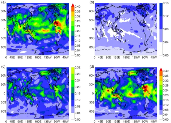
This can be done by comparing Fig. 3 with Fig. 4. Figure 3a displays the AWC map computed from reanalysis data using MIH as an interdependency measure; Fig. 4a dis-plays the AWC map computed from one model run, also us-ing MIH. Clearly, the model is able to capture the same
over--3 -2 -1 0 1 2 3
NINO3.4 anomalies [C] -2
-1 0 1 2
Temperature anomalies [C]
Figure 2.Graphical representation of the linear index-removal
pro-cedure. The SAT anomalies are compared at zero lag with the index (in this case NINO3.4 SST anomalies) and a linear regression is performed (in red).
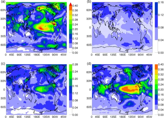
all pattern of global connectivity with a maximum in the cen-tral tropical Pacific, relative maxima in the tropical Atlantic and Indian oceans and over Alaska, the Labrador Sea and the Southern Ocean. Differences are mainly in the magnitude of the AWC, with the model underestimating the connectivity in most places. Similar observation applies to the compari-son between Fig. 3b, c, and d and the corresponding panel in Fig. 4, where the network was built by using the MIOP as an interdependency measure.
Figure 4a shows the AWC using MIH and thus reveals global interdependencies of all the time series; Fig. 4b– d show the AWC using MIOP in intraseasonal, intra-annual and interintra-annual timescales, respectively. Clearly, the connectivity increases as the timescale increases, in good agreement with the results found in Deza et al. (2013) us-ing reanalysis data. Many other features of the AWC maps are also qualitatively well reproduced by the model.
While the networks obtained from AGCM and reanalysis data, when visualized via the AWC, look qualitatively very similar, quantitative differences are seen, for example, with respect to the spatial extent of the structures. These differ-ences might be relevant, especially if more sophisticated net-work measures were to be used. Nevertheless, the good qual-itative agreement between networks constructed from model and reanalysis data lets us focus on using model output to distinguish the networks associated with intrinsic and forced atmospheric variability.
4.2 AWC maps
4.2.1 Forced variability
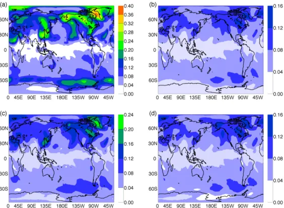
Figure 3. Maps of AWC constructed from reanalysis NCEP/NCAR data. The statistical interdependencies are quantified via (a)MIH, (b)MIOP intraseasonal,(c)intra-annual, and(d)interannual timescales (see Sect. 2.1 for details). The color scale is the same for all panels and for all the following AWC maps.
Figure 4.Maps of AWC obtained from single model run. The statistical interdependencies are quantified via(a)MIH,(b)MIOP
Figure 5.Maps of AWC computed from averaged time series, and thus containing information only of the forced component of atmospheric variability. The quantifiers of statistical similarity are as in Fig. 4:(a)MIH,(b)MIOP intraseasonal,(c)intra-annual, and(d)interannual. It can be noticed that in the shorter timescale the tropical area, especially the Pacific Ocean has a weak influence, and it grows stronger with increasing timescale. The fact that the maps in(a)and(d)are similar suggests that most of the links uncovered by the MIH,(a), actually reflect interdependencies in the longer timescale and thus, are seen in(d).
network from averaged time series (over nine model runs), as explained in Sect. 1.
The results are presented in Fig. 5. Figure 5a displays the AWC map when the MIH is used to quantify statistical in-terdependencies. Here, connectivity is higher in the tropics and on the Pacific, Indian and Atlantic basins than in the rest of the world. It is worth noting that while tropical connecti-vity is relatively symmetrical around the equator for the Pa-cific and Indian oceans, the North Atlantic is significantly more connected than in the south of the equator. Figure 5b–d show that the connectivity of the forced variability increases with the timescale. At intraseasonal timescales connectivity is very low compared with the connectivity from Fig. 5a. If we increase the timescale to intra-annual – as in Fig. 5c – the entire tropical area becomes more connected than the extra-tropics, indicating a better longitudinal energy and momen-tum exchange. Forced by the tropical Pacific SST anoma-lies, a long-range strong teleconnection is found in Alaska (Ropelewski and Halpert, 1987). For interannual timescales (3 years) within the period of the El Niño events (from 2 to 7 years) many very connected areas are found, especially in the tropics but also in the extratropics. The presence of highly connected spots is observed in the extratropics, especially in the Pacific Basin, but also in the Indian and Atlantic oceans.
Comparing these three maps with that in Fig. 5a which, as ex-plained before, was computed via MIH and thus contains in-formation from all the time series, it can be inferred that most of the connections seen in Fig. 5a occur at long timescales, because they are clear only in Fig. 5d, and are weak or not seen in Fig. 5b, c.
Figure 6 represents the same maps as Fig. 5 but after re-moving the NINO3.4 index, as explained in Sect. 3.2. Fig-ures 5a and 6a show large differences. It is clear that the signal of El Niño in the tropical Pacific was successfully re-moved, and moreover, the connection hotspots in the extra-tropics were also removed, indicating that they were mainly forced by El Niño. However, a few small well-connected ar-eas remain over the equatorial Pacific, indicating that a linear regression is not sufficient to fully eliminate the ENSO effect on the network connectivity.
Figure 6.Maps of AWC of the forced component of the network when the index ENSO3.4 is removed from the time series (for the description of the index and for the removal procedure, see Section 3.2). The statistical interdependencies are quantified as in Fig. 4:(a)MIH, MIOP (b) intraseasonal,(c)intra-annual and(d)interannual. A comparison with Fig. 5 allows for an assessment of the influence of El Niño phenomenon over the network connectivity.
might be a reason for the still large connectivity observed in the Caribbean in Fig. 6a.
Other areas, like over China and central Asia, which are weakly connected to the El Niño phenomenon, show the same connectivity in Figs. 5 and 6. The fact that areas not related to ENSO do not change when removing the index hints that the statistical test used to fix the network density is robust and allows us to compare maps with and without the index.
Figure 6b is very similar to Fig. 5b except on the absence of a connected (dark blue) area on the Pacific Ocean, sug-gesting that the influence of El Niño at these timescales is very low and restricted to the tropical Pacific. At intra-annual timescales, Fig. 6c shows the disappearance of many links from the corresponding Fig. 5c. This suggests that at this timescale, even if the El Niño signal is not as strong as on interannual scales, it is already connecting far-away tropical and extratropical areas such as Alaska (Chiang and Sobel, 2002). Thus, removing the El Niño signal very heavily af-fects the connectivity of the network. For longer timescales – shown in Fig. 6d – the scenario is similar as for Fig. 6a with only a remnant of connectivity in the tropical region.
4.2.2 Internal variability
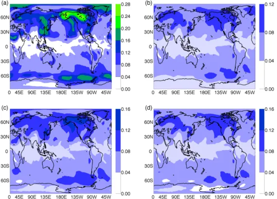
Figure 7 shows AWC maps of internal variability, computed by averaging the nine AWC maps obtained from the indivi-dual model runs, where in each time series, the forced signal (the average of the nine runs) was removed as explained in the Introduction. Contrary to the forced variability case pre-sented before, in this case the most connected areas are on the extratropics. This is consistent with the results of previ-ous figures, and indicates that in the tropics the ocean forces the largest portion of atmospheric variability. As the tropical atmosphere cannot sustain horizontal gradients generated by SST anomalies, it induces vertical movements of air, convec-tion and release of latent heat, thus giving rise to atmospheric circulation anomalies.
In the extratropics internal atmospheric variability is larger, leading to stronger connections. The larger connecti-vity in the Northern Hemisphere suggests that the large land-masses affect atmospheric variability, which is consistent with our current understanding of storm track dynamics and low-frequency transients (James, 1995).
Figure 7.Maps of averaged AWC, revealing the internal variability network (see text for details). The statistical interdependencies are quantified as in Fig. 4(a)MIH, MIOP(b)intraseasonal,(c)intra-annual, and(d)interannual. It can be noticed that in this network, the timescale showing more connectivity is the intra-annual timescale. This is consistent with the shorter memory of the atmosphere compared with the ocean.
– only found using MIH to quantify interdependencies – showed that in this area histograms have a higher skewness than in the rest of the nodes, an effect that has also been re-ported and discussed in Hlinka et al. (2014). This effect is found on the internal-plus-forced AWC map of Fig. 4a, and using reanalysis data as shown in Fig. 3a. When considering other measures to quantify interdependencies, such as Pear-son cross correlation or MIOP, the AWC maps do not show high connectivity in this region (Deza et al., 2013).
With respect to the AWC maps computed by using MIOP, in contrast to the forced case, the intraseasonal, intra-annual and interannual maps are very similar to each other. This is a sign of “multiscale variability”; in other words, variability distributed over many timescales. Internal variability cycles are less well defined, with spectra similar to “red” noise. It can be seen that the most connected AWC map is the intra-annual one, stronger than both the intraseasonal and the in-terannual, consistent with the fact that atmospheric anoma-lies are less persistent than oceanic ones (Hasselmann, 1976; Barsugli and Battisti, 1998).
The fact that the most connected area in Fig. 7a is over the Labrador Sea suggests that it is related to NAO. In order to verify this, we have removed NAO from the time series using the same procedure as with NINO3,4, explained above. The results are shown in Fig. 8. Here, indeed the Labrador con-nected area disappears in all the panels, while the
connecti-vity unrelated to NAO (i.e., over the Southern Hemisphere or China) remains almost unchanged.
4.3 Node connectivity maps
AWC maps provide information about the connectivity of the geographical regions, but no information about the nature – spatial range or distribution – of the links. It is expected that nearby points behave similarly and this leads to high values of correlation between nearby places (Radebach et al., 2013; Donges et al., 2009a). The distance over which the climate variables are well connected is related with the Rossby ra-dius of deformation (RRD) (James, 1995), which is the dis-tance that a particle or wave travels before being significantly affected by the earth’s rotation. Also, in the tropics, this prox-imity effect can be greatly enhanced, as there the information is propagated very fast longitudinally. Here we are interested in unveiling the presence of teleconnections, that is, connec-tions between regions separated by more than the RRD.
Figure 8.Maps of averaged AWC, revealing the internal variability network when the NAO index is removed from the time series (see Sect. 3.2 for details). The statistical interdependencies are quantified as in Fig. 4(a)MIH, MIOP(b)intraseasonal,(c)intra-annual, and (d)interannual. It can be noticed that in this network the timescale showing more connectivity is the intra-annual timescale. This is consistent with the shorter memory of the atmosphere compared with the ocean.
way we are able to see the weak links with good resolution, losing information for the stronger links (stronger than 0.3 on the arbitrary scale of MI, where the highest links have values of 1 or 2 on the same scale, as shown in Deza et al., 2013) which will be all represented with the same color.
4.3.1 Forced variability
Figure 9 shows the connections of a point in the central Pa-cific Ocean in the forced variability network. It is clear from the comparison of the maps in the first row that most links are interannual links.
Figure 9c and d display the same node connectivity maps as in Fig. 9a and b respectively, however, in this case the NINO3.4 index has been removed from the time series and thus (to first order) they do not contain links due to El Niño phenomenon. The differences between Fig. 9a and Fig. 9c and between Fig. 9b and Fig. 9d are evident. First, after elim-inating the effects of El Niño the tropical and extratropical teleconnection patterns associated to the spot in the Pacific disappear independently of the methodology used to quan-tify interdependencies (MIH or MIOP): the connectivity be-comes restricted to the tropical Pacific Basin. Even inside this region the connectivity is greatly decreased as seen by a much smaller red spot of links over 0.3, although the re-maining connections indicate that, either a linear regression
is not enough to fully remove the influence of El Niño, or the ENSO dynamics is not fully represented by the NINO3.4 index.
According to Fig. 9a and b, Alaska is an area well con-nected to the equatorial Pacific Ocean. To further investigate, Fig. 10 shows global connections to a point near Alaska. It can be seen in Fig. 10a and b that it indeed presents connec-tions to the equatorial Pacific Ocean with a maximum close to the dateline.
Furthermore, connections to the southern Pacific Ocean, Central Africa, Indian Ocean and even the Drake Passage are found. These connections are stronger in Fig. 10b, especially those linking Alaska with the Indian and southern Atlantic Ocean and the Drake Passage. If we remove NINO3.4 we find a dramatic change in the maps. Connections become al-most local and all the north–south teleconnections are lost; only connections probably associated with an imperfect re-moval of the El Niño signal remain. This indicates that there are no direct teleconnections between Alaska and (for exam-ple) the Drake Passage, but both are strongly connected to El Niño. As these networks are constructed using symmet-rical measures of dependency, calculated directly from the data, they are unable to distinguish between a direct connec-tion and an indirect one.
Figure 9.Connectivity map of a node in the central Pacific (indicated with X). Panels(a)and(b)are computed from forced time series (averaging over nine model realizations); panels(c)and(d)are also computed from forced time series, but with ENSO3.4 linearly removed and thus not containing – to the first order – contributions due to El Niño. In(a),(c)interdependencies are quantified via MIH; in(b),(d)via MIOP interannual timescale.
Figure 10.As Fig. 9 but regarding a node near Alaska (indicated with X). Compared to Fig. 9 one can notice that the teleconnection between
Figure 11.As Fig. 9 but regarding a node near New Zealand (indicated with X). In panels(b)and(d)the MIOP is adjusted to interannual timescale. Compare with Figs. 9 and 10.
Zealand because it shows a relatively high forced density (seen in Fig. 5a, b) and it is connected to the selected point over the tropical Pacific of Fig. 9a, b. Figure 11a shows connectivity between the chosen point and the Pacific and Indian oceans, as well as wave patterns (probably a Rossby wave train) along the extratropics. Figure 11b adds informa-tion to Fig. 11a, showing that these teleconnecinforma-tions are of in-terannual type. If we remove NINO3.4 (Fig. 11c, d) not sur-prisingly the links to the tropical Pacific disappear, but also some of the connectivity to the Indian Ocean, suggesting that part of the links with the Indian Ocean are indirect. Never-theless, the extra-tropical wave train remains, and Fig. 11d suggests that the wave train may be forced by the Indian Ocean at interannual timescales. As in the previous figure, some weak north–south teleconnections are found, but they disappear if we remove the NINO3.4 index, indicating again an indirect connection between the extratropics through the Pacific Ocean.
4.3.2 Internal variability
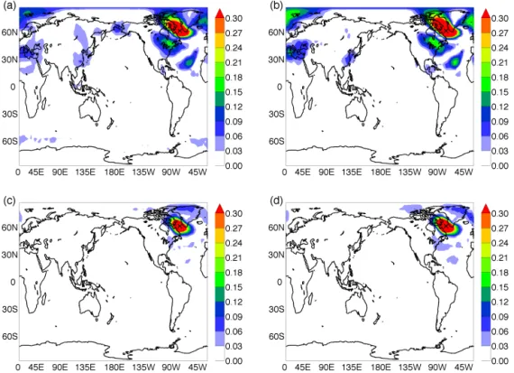
Figure 12 displays theinternal variability connections of a node over the most connected area of Fig. 7. The average of the resulting nine different connectivity maps is shown. In the left column the connectivity computed using MIH is displayed, while in the right column, the intra-annual scale is shown, using MIOP. This timescale shows the strongest response for internal variability. In Fig. 12a the original
in-ternal variability connections are shown, revealing telecon-nections extending over the Northern Hemisphere, especially over Scandinavia, Mediterranean Europe, the east coast of North America and the tropical North Atlantic. Figure 12a also shows connections to eastern China and the Aleutian is-lands. The pattern shown in Fig. 12b mainly corresponds to the known influence of the North Atlantic Oscillation. This is further substantiated in Fig. 12c and d of the same figure, where the NAO influence is removed and the connections of the Labrador Sea, particularly in the northern Atlantic Basin, are strongly weakened.
5 Summary and conclusions
Figure 12.Maps of internal variability showing the connectivity of a node in the Labrador Sea (indicated with X). Panels(a)and (b) correspond to the original internal time series as in Fig. 7; in panels(c)and(d)the NAO was linearly removed and thus the links do not contain – to the first order – contributions due to the North Atlantic Oscillation. In(a)and(c)interdependencies are quantified via MIH; in (b)and(d)via MIOP intra-annual timescale.
series. Ordinal patterns have been used in order to separate and determine the strength of the links at different timescales. While the main conclusions of our analysis (the connecti-vity of the forced variability network is heavily affected by El Niño, whereas that of the internal variability network is significantly affected by the NAO) are not new, new infor-mation has been uncovered, as ordinal analysis allows us to study these phenomena on different timescales. This has revealed that most of the links detected in the forced va-riability proceed from long timescales, while the contribu-tions of intra-annual timescales to the internal variability are the most important. This work also opens the possibility of studying how various network measures, such as the average path length, assortativity, clustering coefficient, betweeness, etc. depend on the timescale considered for quantifying sta-tistical interdependencies.
Another conclusion of this work is that forced and inter-nal atmospheric variability are characterized by very differ-ent networks. Because the separation of internal and forced variability done here requires averaging over several model runs, the networks obtained here could not have been ob-tained from observational/reanalysis data only. It is shown that the forced variability is stronger in the tropics, while the internal variability peaks in the mid-latitudes. The network of forced variability has the strongest connections at interan-nual timescales.Long-range teleconnectionsfrom the tropics
to the extratropics and even from different hemispheres in the forced network were observed and explained by the influence of El Niño. On the other hand, the network of internal atmo-spheric variability has the strongest connections in the extrat-ropics, and it was found that connections to the Labrador Sea are heavily affected by the North Atlantic Oscillation.
This study is focused on the lowest levels of the atmo-sphere. A complementary analysis is performed in the com-panion paper by Arizmendi et al. (2014), devoted to the study of the evolution of the upper atmosphere during the 20th century and aiming at distinguishing the oceanically forced component from the atmospheric internal variability on dif-ferent timescales. The methodology proposed here for dis-tinguishing links in spatial range (short and long), timescale (intraseasonal, intra-annual and interannual) and type of va-riability (forced vs. internal) is a novel approach for the study of climate networks that provides new insight into the clima-tological meaning of the links found, and their connection to physical phenomena.
Gestió d’Ajuts Universitaris i de Recerca (AGAUR), Generalitat de Catalunya, and the ICREA ACADEMIA award.
Edited by: R. Donner
Reviewed by: D. Handorf and one anonymous referee
References
Albert, R. and Barabási, A. L.: Statistical mechanics of complex networks, Rev. Mod. Phys., 74, 47–97, doi:10.1103/RevModPhys.74.47, 2002.
Allen, M. R., and Smith L. A.: Optimal filtering in singular spec-trum analysis, Phys. Lett. A, 234, 419–428, doi:10.1016/S0375-9601(97)00559-8, 1997.
Amigó, J. M.: Topological permutation entropy, Springer Berlin Heidelberg, 2010.
Arizmendi, F., Martí, A., and Barreiro, M.: Evolution of atmo-spheric connectivity in the 20th century, accepted, Nonlin. Pro-cesses Geophys., 2014.
Bandt, C. and Pompe, B.: Permutation entropy: A natural com-plexity measure for time series, Phys. Rev. Lett., 88, 174102, doi:10.1103/PhysRevLett.88.174102, 2002.
Barreiro, M.: Influence of ENSO and the South Atlantic Ocean on climate predictability over Southeastern South America, Clim. Dynam., 35, 1493–1508, doi:10.1007/s00382-009-0666-9, 2009. Barreiro, M. and Díaz, N.: Land-atmosphere coupling in El Niño influence over South America, Atmos. Sci. Lett., 12, 351–355, doi:10.1002/asl.348, 2011.
Barreiro, M., Chang, P., and Saravanan, R.: Variability of the South Atlantic Convergence Zone as simulated by an atmo-spheric general circulation model, J. Climate, 15, 745–763, doi:10.1175/1520-0442(2002)015<0745:VOTSAC>2.0.CO;2, 2002.
Barreiro, M., Chang, P., Ji, L., Saravanan, R., and Giannini, A.: Dy-namical Elements of Predicting Boreal Spring Tropical Atlantic Sea-Surface Temperatures, Dynam. Atmos. Oceans, 39, 69–85, doi:10.1016/j.dynatmoce.2004.10.013, 2005.
Barreiro, M., Martí, A. C., and Masoller, C.: Inferring long mem-ory processes in the climate network via ordinal pattern analysis, Chaos, 21, 013101, doi:10.1063/1.3545273, 2011.
Barsugli, J. J. and Battisti, D. S.: The Basic Effects of Atmosphere–Ocean Thermal Coupling on Midlatitude Va-riability, J. Atmos. Sci., 55, 477–493, doi:10.1175/1520-0469(1998)055<0477:TBEOAO>2.0.CO;2, 1998.
Bracco, A., Kucharski, F., Kallummal, R., and Molteni, F.: Internal variability, external forcing and climate trends in multi-decadal AGCM ensembles, Clim. Dynam., 23, 659–678, doi:10.1007/s00382-004-0465-2, 2004.
Chang, P., Saravanan, R., Ji, L., and Hegerl, G. C.: The effect of local sea surface temperatures on atmospheric circulation over the tropical Atlantic sector, J. Climate, 13, 2195–2216, doi:10.1175/1520-0442(2000)013<2195:TEOLSS>2.0.CO;2, 2000.
Chiang, J. C. H. and Sobel, A. H.: Tropical tropospheric tempera-ture variations caused by ENSO and their influence on the remote tropical climate, J. Climate, 15, 2616–2631, doi:10.1175/1520-0442(2002)015<2616:TTTVCB>2.0.CO;2, 2002.
Cover, T. M. and Thomas, J. A.: Elements of information theory, John Wiley & Sons, 2006.
Deza, J. I., Barreiro, M., and Masoller, C.: Inferring interdependen-cies in climate networks constructed at interannual, intra–season and longer time scales, Eur. Phys. J.-Spec. Top., 222, 511–523, doi:10.1140/epjst/e2013-01856-5, 2013.
Donges, J. F., Zou, Y., Marwan, N., and Kurths, J.: Complex net-works in climate dynamics, Eur. Phys. J.-Spec. Top., 174, 157– 179, doi:10.1140/epjst/e2009-01098-2, 2009a.
Donges, J. F., Zou, Y., Marwan, N., and Kurths, J.: The back-bone of the climate network, EPL-Europhys. Lett., 87, 48007, doi:10.1209/0295-5075/87/48007, 2009b.
Frankignoul, C. and Hasselmann, K.: Stochastic climate models, Part II Application to sea-surface temperature anomalies and thermocline variability, Tellus, 29, 289–305, doi:10.1111/j.2153-3490.1977.tb00740.x, 1977.
Gámez, A. J., Zhou, C. S., Timmermann, A., and Kurths, J.: Nonlin-ear dimensionality reduction in climate data, Nonlin. Processes Geophys., 11, 393–398, doi:10.5194/npg-11-393-2004, 2004. Gozolchiani, A., Havlin, S., and Yamasaki, K.: Emergence of El
Niño as an autonomous component in the climate network, Phys. Rev, Lett., 107, 148501, doi:10.1103/PhysRevLett.107.148501, 2011.
Hasselmann, K.: Stochastic climate models part I. Theory, Tellus, 28, 473–485, doi:10.1111/j.2153-3490.1976.tb00696.x, 1976. Hlinka, J., Hartman, D., Vejmelka, M., Runge, J., Marwan, N.,
Kurths, J., and Paluš, M.: Reliability of inference of directed cli-mate networks using conditional mutual information, Entropy, 15, 2023–2045, doi:10.3390/e15062023, 2013.
Hlinka, J., Hartman, D., Vejmelka, M., Novotná, D., and Paluš, M.: Non-linear dependence and teleconnections in climate data: sources, relevance, nonstationarity, Clim. Dynam., 42, 1873– 1886, doi:10.1007/s00382-013-1780-2, 2014.
Hurrell, J. W.: Decadal trends in the North Atlantic oscillation: Re-gional temperatures and precipitation, Science, 269, 676–679, doi:10.1126/science.269.5224.676, 1995.
James, I. N.: Introduction to circulating atmospheres, Cambridge University Press, 1995.
Kalnay E., Kanamitsu, M., Kistler, R., Collins, W., Deaven, D., Gandin, L., Iredell, M., Saha, S., White, G., Woollen, J., Zhu, Y., Leetmaa, A., Reynolds, R., Chelliah, M., Ebisuzaki, W., Hig-gins, W., Janowiak, J., Mo, K. C., Ropelewski, C., Wang J., Jenne, R., and Joseph, D.: The NCEP/NCAR 40-Year Reanalysis Project, B. Am. Meteorol. Soc., 77, 437–471, doi:10.1175/1520-0477(1996)077<0437:TNYRP>2.0.CO;2, 1996.
Kucharski, F., Molteni, F., and Bracco, A.: Decadal interactions be-tween the Western Tropical Pacific and the North Atlantic Oscil-lation, Clim. Dynam., 26, 79–91, doi:10.1007/s00382-005-0085-5, 2005.
Lind, P. G., Mora, A., Gallas, J. A., and Haase, M.: Re-ducing stochasticity in the North Atlantic Oscillation index with coupled Langevin equations, Phys. Rev. E, 72, 056706, doi:10.1103/PhysRevE.72.056706, 2005.
Malik, N., Bookhagen, B., Marwan, N., and Kurths, J.: Analy-sis of spatial and temporal extreme monsoonal rainfall over South Asia using complex networks, Clim. Dynam., 39, 971– 987, doi:10.1007/s00382-011-1156-4, 2012.
Molteni, F.: Atmospheric simulations using a GCM with simplified physical parametrizations. I: model climatology and variability in multi-decadal experiments, Clim. Dynam., 20, 175–191, doi:10.1007/s00382-002-0268-2, 2003.
NOAA: website available at: http://www.esrl.noaa.gov/psd/data/ climateindices/list/, last access: 31 October 2013, 2013. Paluš, M.: From Nonlinearity to Causality: Statistical
test-ing and inference of physical mechanisms underly-ing complex dynamics, Contemp. Phys., 48, 307–348, doi:10.1080/00107510801959206, 2007.
Paluš, M., Hartman, D., Hlinka, J., and Vejmelka, M.: Discerning connectivity from dynamics in climate networks, Nonlin. Pro-cesses Geophys., 18, 751–763, doi:10.5194/npg-18-751-2011, 2011.
Pohlmann, H. and Latif, M.: Atlantic versus Indo-Pacific influence on Atlantic-European climate, Geophys. Res. Lett., 32, 05707, doi:10.1029/2004GL021316, 2005.
Pompe, B. and Runge, J.: Momentary information transfer as a coupling measure of time series, Phys. Rev. E, 83, 051122, doi:10.1103/PhysRevE.83.051122, 2011.
Radebach, A., Donner, R. V., Runge, J., Donges, J. F., and Kurths, J.: Disentangling different types of El Niño episodes by evolving climate network analysis, Phys. Rev. E, 88, 052807, doi:10.1103/PhysRevE.88.052807, 2013.
Rodwell, M. J., Rowell, D. P., and Folland, C. K.: Oceanic forc-ing of the wintertime North Atlantic Oscillation and European climate, Nature, 398, 320–323, doi:10.1038/18648, 1999. Ropelewski, C. F. and Halpert, M. S.: North American precipitation
and temperature patterns associated with the El Niño–Southern Oscillation (ENSO), Mon. Weather Rev., 114, 2352–2362, doi:10.1175/1520-0493(1986)114<2352:NAPATP>2.0.CO;2, 1986.
Schreiber, T. and Schmitz, A.: Improved Surrogate Data for Nonlinearity Tests, Phys. Rev. Lett., 77, 635–638, doi:10.1103/PhysRevLett.77.635, 1996.
Seager, R., Naik, N., Baethgen, W., Robertson, A., Kushnir, Y., Nakamura, J., and Jurburg, S.: Tropical Oceanic Causes of In-terannual to Multidecadal Precipitation Variability in Southeast South America over the Past Century, J. Climate, 23, 5517–5539, doi:10.1175/2010JCLI3578.1, 2010.
Shukla, J.: Predictability in the midst of chaos: a scien-tific basis for climate forecasting, Science, 282, 728–731, doi:10.1126/science.282.5389.728, 1998.
Smith, T. M. and Reynolds, R. W.: Improved extended recon-struction of SST (1854–1997), J. Climate, 17, 2466–2477, doi:10.1175/1520-0442(2004)017<2466:IEROS>2.0.CO;2, 2004.
Straus, D. M. and Shukla, J.: Distinguishing between the SST-forced variability and internal variability in mid latitudes: anal-ysis of observations and GCM simulations, Q. J. Roy. Meteor. Soc., 126, 2323–2350, doi:10.1002/qj.49712656716, 2000. Ting, M., Kushnir, Y., Seager, R., and Li, C.: Forced and internal
twentieth-century SST Trends in the North Atlantic, J. Climate, 22, 1469–1481, doi:10.1175/2008JCLI2561.1, 2009.
Tirabassi, G. and Masoller, C.: On the effects of lag-times in networks constructed from similarities of monthly fluc-tuations of climate fields, EPL-Europhys. Lett., 102, 59003, doi:10.1209/0295-5075/102/59003, 2013.
Trenberth, K. E.: The Definition of El Niño, B. Am. Meteorol. Soc., 78, 2771–2777, doi:10.1175/1520-0477(1997)078<2771:TDOENO>2.0.CO;2, 1997.
Trenberth, K. E., Branstator, G. W., Karoly, D., Kumar, A., Lau, N. C., and Ropelewski, C.: Progress during TOGA in understand-ing and modelunderstand-ing global teleconnections associated with tropical sea surface temperatures, J. Geophys. Res., 103, 14291–14324, doi:10.1029/97JC01444, 1998.
Tsonis, A. A. and Swanson, K. L.: Review article “On the ori-gins of decadal climate variability: a network perspective”, Non-lin. Processes Geophys., 19, 559–568, doi:10.5194/npg-19-559-2012, 2012.
Tsonis, A. A., Swanson, K. L., and Roebber, P. J.: What do networks have to do with climate?, B. Am. Meteorol. Soc., 87, 585–595, doi:10.1175/BAMS-87-5-585, 2006.
Tsonis, A. A., Swanson, K. L., and Wang, G.: On the role of atmo-spheric teleconnections in climate, J. Climate, 21, 2990–3001, doi:10.1175/2007JCLI1907.1, 2008.
van der Mheen, M., Dijkstra, H. A., Gozolchiani, A., den Toom, M., Feng, Q. Y., Kurths, J., and Hernandez Garcia, E.: In-teraction network based early warning indicators for the At-lantic MOC collapse, Geophys. Res. Lett., 40, 2714–2719, doi:10.1002/grl.50515, 2013.
Venzke, S., Allen, M. R., Sutton, R. T., and Rowell, D. P.: The atmospheric response over the North Atlantic to decadal changes in sea surface temperature, J. Climate, 12, 2562–2584, doi:10.1175/1520-0442(1999)012<2562:TAROTN>2.0.CO;2, 1999.