www.atmos-chem-phys.net/13/6207/2013/ doi:10.5194/acp-13-6207-2013
© Author(s) 2013. CC Attribution 3.0 License.
Atmospheric
Chemistry
and Physics
Geoscientiic
Geoscientiic
Geoscientiic
Geoscientiic
Effect of land cover on atmospheric processes and air quality
over the continental United States – a NASA Unified
WRF (NU-WRF) model study
Z. Tao1,2, J. A. Santanello2, M. Chin2, S. Zhou2,3, Q. Tan1,2, E. M. Kemp2,4, and C. D. Peters-Lidard2 1Universities Space Research Association, 10211 Wincopin Circle, Columbia, MD 21044, USA
2NASA Goddard Space Flight Center, Greenbelt, MD 20771, USA 3Northrop Grumman Information System, McLean, VA 22102, USA 4Science System and Applications, Inc., Lanham, MD 20706, USA Correspondence to:Z. Tao ([email protected])
Received: 20 December 2012 – Published in Atmos. Chem. Phys. Discuss.: 27 February 2013 Revised: 24 May 2013 – Accepted: 28 May 2013 – Published: 1 July 2013
Abstract. The land surface plays a crucial role in regulat-ing water and energy fluxes at the land–atmosphere (L–A) interface and controls many processes and feedbacks in the climate system. Land cover and vegetation type remains one key determinant of soil moisture content that impacts air temperature, planetary boundary layer (PBL) evolution, and precipitation through soil-moisture–evapotranspiration cou-pling. In turn, it will affect atmospheric chemistry and air quality. This paper presents the results of a modeling study of the effect of land cover on some key L–A processes with a focus on air quality. The newly developed NASA Unified Weather Research and Forecast (NU-WRF) modeling system couples NASA’s Land Information System (LIS) with the community WRF model and allows users to explore the L– A processes and feedbacks. Three commonly used satellite-derived land cover datasets – i.e., from the US Geological Survey (USGS) and University of Maryland (UMD), which are based on the Advanced Very High Resolution Radiome-ter (AVHRR), and from the Moderate Resolution Imaging Spectroradiometer (MODIS) – bear large differences in agri-culture, forest, grassland, and urban spatial distributions in the continental United States, and thus provide an excellent case to investigate how land cover change would impact at-mospheric processes and air quality. The weeklong simu-lations demonstrate the noticeable differences in soil mois-ture/temperature, latent/sensible heat flux, PBL height, wind, NO2/ozone, and PM2.5air quality. These discrepancies can be traced to associate with the land cover properties, e.g.,
stomatal resistance, albedo and emissivity, and roughness characteristics. It also implies that the rapid urban growth may have complex air quality implications with reductions in peak ozone but more frequent high ozone events.
1 Introduction
index (LAI) impacts the partition of surface heat fluxes and regulates light extinction within the canopy that directly af-fects the leaf stomatal conductance. LAI and stomatal resis-tance (RS) parameters are required to estimate the canopy resistance, which, together with the green vegetation frac-tion (SHDFAC), is subsequently used to calculate plant ET (Seneviratne et al., 2010; Kumar et al., 2011) that determines the water cycle in the land–biosphere–atmosphere system. Generally, the canopy resistance is positively proportional to RS but negatively to LAI. Large canopy resistance leads to small ET (Kumar et al., 2011) and slows dry deposition of an atmospheric species (Charusombat et al., 2010). Surface roughness length (Z0) parameterizes the roughness charac-teristics of the terrain and affects the intensity of mechanical turbulence and fluxes of various quantities above the surface. Urban and forest LULCs bear highZ0 values that tend to reduce the near-surface wind speed.
Since the pioneering work by Deardorff (1978), who de-veloped the first detailed parameterization of the land surface that was efficient enough to be applied in the atmospheric numerical simulation, many studies have been carried out to investigate the land surface effect on boundary layer meteo-rology and, more recently, on air quality. For example, Sun and Bosilovich (1996) examined the sensitivity of boundary layer meteorology to the selection of land surface parame-ters – e.g., vegetation cover, minimum RS,Z0, and initial SM – and found out that the SM gave the largest impact on the PBL height (PBLH) and surface heat budget. Kohler et al. (2010) studied the impact of SM on boundary layer char-acteristics – e.g., temperature and PBLH – using the observa-tions from the African Monsoon Multidisciplinary Analysis (AMMA) campaign. Santanello et al. (2011) used a “process chain” to describe how SM affected the precipitation. Cheng et al. (2008) demonstrated that the accurate representation of land surface properties was crucial to modeling the realis-tic meteorology and air quality with a model study focused on the Houston-Galveston metropolitan areas. Ganzeveld et al. (2010) investigated the impacts of LULC changes on at-mospheric chemistry at a global scale and found that the overall influence on reactive trace-gas exchanges was not very large due to the compensation effects; for example, the reduction in soil NO emissions from tropical forest clearing was made up for by a decrease in NO2foliage uptake.
Though impacts of the land surface on PBL and chemistry processes have been demonstrated in these studies, the prac-tical issue of how to best represent these processes in coupled models remains unresolved. In particular, the vast arrays of land surface schemes often use different land cover datasets that are applied at different spatial resolutions. This makes intercomparison across different models or even within mod-els of different versions and datasets untenable. This issue will only grow in importance as the number of satellite-derived datasets continues to increase along with the model complexity. To this end, this study addresses the LULC im-pacts on atmospheric processes and air quality from a
differ-ent perspective. Instead of arbitrarily adjusting land surface parameters or relying on models to project LULC changes, this study employs three widely used and observation-driven LULC datasets within one modeling system. These three datasets are from the US Geological Survey (USGS, Love-land et al., 2000) and University of MaryLove-land (UMD, Hansen et al., 2000), which are based on the Advanced Very High Resolution Radiometer (AVHRR), and from the Moderate Resolution Imaging Spectroradiometer (MODIS, Friedl et al., 2002). They display a large discrepancy in LULC clas-sification and distribution, and provide an excellent proxy case to investigate how LULC and its change would affect the atmospheric chemistry. The newly developed NASA Uni-fied Weather Research and Forecasting (NU-WRF) model-ing system is used to explore this, utilizmodel-ing the flexible land surface model (LSM) interface of NASA’s Land Information System (LIS, Kumar et al., 2006; Peters-Lidard et al., 2007). The paper presents the model, LULC data, and experimen-tal design details in Sect. 2. Section 3 then follows with re-sults of the most relevant parameters (e.g., SM, surface tem-perature, wind, and PBLH), followed by the analysis of the land surface emissions, dry deposition, and air quality focus-ing on ozone chemistry. Lastly, the implication of urbaniza-tion to air quality is briefly discussed, followed by the sum-mary and conclusions.
2 NU-WRF modeling system and evaluation
2.1 Model description
conditions on a common grid to initialize NU-WRF, and al-low various plug-ins such as land data assimilation, param-eter estimation, and uncertainty analysis (Santanello et al., 2011, 2013). LIS can be run both in offline and coupled mode for NU-WRF. The major advantages of this model-ing arrangement are multifold (Kumar et al., 2008). First, LIS is capable of conducting a long-term offline “spin-up” to allow the land surface and soil profiles to reach thermody-namic equilibrium, which otherwise is impossible in WRF. The initial soil conditions rendered by this long-term offline LIS spin-up resulted in an improved simulation of timing and evolution of a sea-breeze circulation over portions of north-western Florida (Case et al., 2008). Case et al. (2011) also investigated the impact of a LIS spin-up on summertime pre-cipitation over the southeastern US. They found that the near-surface SM was improved in the spin-up, and that there was measurable impact of the spin-up on the coupled near-surface and PBL conditions relative to that using the default land ini-tialization via WRF. Second, the offline LIS can be run us-ing the same LSM and at the same resolution as the online version, thus making the data internally consistent and elim-inating the need for horizontal spatial interpolation. Last but not the least, the LIS framework allows users to introduce new ancillary datasets (e.g., land cover, soil type, vegetation condition) into NU-WRF, which makes this study possible.
2.2 Experimental design and model set-up
Three sets of NU-WRF simulations have been carried out with the identical physics, gas and aerosol chemistry, emis-sions, and meteorological and chemical lateral boundary conditions but different LULC representation. The key com-mon options for NU-WRF modeling are the Goddard micro-physics and the long/short-wave radiation scheme, LIS as the land surface component (Kumar et al., 2008), the Monin– Obukhov surface layer scheme, the Yonsei University plane-tary boundary layer scheme (YSU, Hong et al., 2006), the new Grell cumulus scheme – an improved Grell–Devenyi ensemble cumulus scheme (Grell and Devenyi, 2002) that allows subsidence spreading for high-resolution simulation (Lin et al., 2010), the second generation regional acid de-position model (RADM2, Stockwell et al., 1990; Gross and Stockwell, 2003) gas-phase chemical mechanism, and the GOCART aerosol scheme. Over a multiyear spin-up, LIS generates the physical states of soil moisture and soil tem-perature that are then fed into NU-WRF as the initial land surface conditions. The LIS spin-up improves upon common approaches of employing coarse atmospheric data initializa-tion of the land surface and of using a “cold-start” initial con-dition.
To investigate the effect of LULC on atmospheric pro-cesses and air quality, three commonly used LULC datasets from USGS, UMD, and MODIS have been applied within the LIS framework to the Noah LSM (Ek et al., 2003) version 3.2
with the corresponding NU-WRF experiments designated as E USGS, E UMD, and E MODIS, respectively.
Within the Noah LSM, the State Soil Geographic (STATSGO, Miller and White, 1998) soil texture database, along with the three LULC datasets, were applied. The at-mospheric forcing data for the spin-up period were provided by the North American Land Data Assimilation System (NL-DAS, Mitchell et al., 2004). Rodell et al. (2005) examined the sensitivity (and in turn, requirements) of equilibration to the length of the spin-up run, which was found to vary with different climate regimes (e.g., cold and dry regions tended to take longer to equilibrate than warm and moist locales) and soil type, but that a 3–4 yr spin-up was sufficient in most cases. Case et al. (2008), who applied LIS-WRF to weather forecast, found that a 2 yr offline spin-up was warranted to ensure convergence to a soil state equilibrium. Following the findings, the offline LIS was run for 3.5 yr leading to 26 May 2010. The output from the LIS spin-up was then used to ini-tialize soil temperature and soil moisture in NU-WRF sim-ulations. In the coupled simulation, the NU-WRF-generated atmospheric forcing variables drove the Noah LSM within LIS to produce surface energy and water fluxes that were fed back into NU-WRF at each time step. In this manner, a con-sistent LSM configuration was employed in both NU-WRF and offline LIS.
Anthropogenic emissions in this study were from the 2005 National Emissions Inventory compiled by the US Envi-ronmental Protection Agency (http://www.epa.gov/ttnchie1/ net/2005inventory.html, USEPA). Fire emissions were from the Global Fire Data version 3 (GFED3, van der Werf et al., 2010; Mu et al., 2011). Biogenic emissions were cal-culated online using the Model of Emissions of Gases and Aerosols from Nature version 2 (MEGAN2, Guenther et al., 2006). Dust emissions were estimated online based on the surface wind speed, soil moisture, and soil erodibility map that was originally generated for global model GOCART (Ginoux et al., 2001) and updated with higher spatial reso-lution (0.25◦×0.25◦).
Table 1.Percentage agreements of MODIS/USGS, MODIS/UMD, and USGS/UMD for eight common land classifications.
Land Category MODIS and USGS (%) MODIS and UMD (%) USGS and UMD (%)
Evergreen Needleleaf Forest 76.2 62.3 46.3 Evergreen Broadleaf Forest 0.3 9.6 3.1 Deciduous Broadleaf Forest 67.3 56.9 38.3
Mixed Forests 51.3 37.5 34.5
Barren or Sparsely Vegetated 42.0 63.9 91.3
Grasslands 43.4 47.0 57.0
Urban and Built-up Land 36.7 44.3 96.3
Croplands 64.3 72.1 53.3
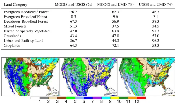
Fig. 1.LULC maps from USGS, UMD, and MODIS. 1 (grey) represents barren or sparsely vegetated land; 2, croplands; 3, cropland/natural land mosaic; 4, grasslands; 5, open shrubland; 6, closed shrubland; 7, woodland; 8, mixed forests; 9, deciduous broadleaf forest; 10, evergreen needleleaf forest; 11, evergreen broadleaf forest; 12 (red), urban and built-up land.
2.3 LULC data
Three LULC datasets from USGS, UMD, and MODIS have been applied to the CONUS domain at a 20 km resolution using a dominant class aggregation approach from the native 1 km resolution data. The USGS and UMD data were both derived from the AVHRR satellite measurements based on the maximum monthly normalized difference vegetation in-dex (NDVI) composites collected from April 1992 through March 1993 (Hansen and Reed, 2000). While the USGS data were created using the 12-monthly maximum NDVI values as the inputs into an unsupervised clustering algorithm, the UMD data were based on all five AVHRR channels (rang-ing from 0.58 to 12.5 µm) and the NDVI that were used to derive the 41 multitemporal metrics with a supervised clas-sification tree algorithm. The MODIS data were also derived using a supervised classification method that relied on both a global site database and the spectral information collected by MODIS. It was based on the collection four MODIS/Terra data from the period of 1 January to 31 December 2001 (http: //duckwater.bu.edu/lc/mod12q1.html). The system for terres-trial ecosystem parameterization was developed and applied to create the global site database to serve as the training sites for MODIS land classification estimate and evaluation. Spec-tral information from MODIS’s seven land bands and the en-hanced vegetation index product were used to provide the amount and fractional cover of live vegetation within each pixel. It should be noted that this study is not intended to
as-sess the LULC in a particular year but to examine the impact of different LULC on air quality. Therefore, the data based on different satellite sensors/methods and different years would provide the necessary LULC contrast for the purpose.
Table 1 shows the percentage of areas in agreement for the eight land categories that are commonly labeled for all three datasets. It can be seen that in the areas designated as ever-green needleleaf forest in MODIS, only 76.2 % bear the same category in USGS and 62.3 % in UMD. The discrepancies for the evergreen broadleaf forest are especially large, prob-ably because the overall area of this category is small and the algorithms employed in three datasets are insensitive to distinguishing it in the CONUS domain. The agreement be-tween USGS and UMD for urban and built-up land is more than 95 % largely because both UMD and USGS datasets adopt this land type from the populated places’ data layer in the Digital Chart of the World (Danko, 1992). Combin-ing these eight land categories together, the overall agree-ments of MODIS/USGS and MODIS/UMD are 55.8 % and 53.7 %, respectively. The overall agreement between USGS and UMD stands at 47.8 %.
from UMD, and cropland/natural vegetation mosaic from MODIS); (2) open shrubland (mixed shrubland/grassland and savanna from USGS, open shrublands from UMD, and open shrublands and savanna from MODIS); (3) closed shrubland (shrubland from USGS, wooded grassland and closed shrublands from UMD, and closed shrublands and woody savannas from MODIS); and (4) woodland (wooded wetland and wooded tundra from USGS, woodland from UMD, and none from MODIS). Figure 1 shows the spa-tial distributions of the comparison. Both UMD and MODIS replace the large portions of open shrubland designated in USGS in the Central Valley of California with croplands. In comparison to USGS and MODIS, UMD replaces the large portions of cropland and natural land mosaic with closed shrubland from northwestern to southeastern Minnesota; the large portions of cropland with closed shrubland along the border of Iowa and Missouri; the large potions of croplands, grasslands, and open shrubland with closed shrubland in eastern Kansas, central Oklahoma, and eastern Texas; and the large portions of cropland and cropland mosaic with closed shrubland in the central Florida. Compared with USGS and UMD, MODIS expands the urban and built-up land to twice as much. These LULC differences among the three datasets would cause large impacts on atmospheric processes and air quality, as will discussed in the following sections.
The LULC influences the atmospheric processes and air quality through the various parameters pre-set in NU-WRF. For example, soil moisture (SM) plays a key role in regulat-ing the land water and energy balances, as well as in affectregulat-ing the exchanges of trace gases and particles between land and atmosphere (Seneviratne et al., 2010). Its estimate in NU-WRF is based on a series of LULC parameters. Conceptually, Eq. (1) governs the land surface water mass balance:
dSM
dt =P−ET−SR−D, (1)
whereP is the precipitation, ET is the evapotranspiration, SR denotes for the surface runoff, andDis the drainage. Equa-tions (2) through (4) depict the land surface energy balance:
dE
dt =Rn−LH−HFX−GFX (2)
Rn=(1−albedo)·SWin+LWin−LWout (3)
LWout=emissivity·σ·T4, (4)
where Rn is the net radiation on surface as a function of surface albedo, incoming short-wave (SWin) and longwave (LWin) radiation, and outgoing longwave radiation (LWout). LH is the latent heat flux, HFX is the sensible heat flux, and GFX is the ground heat flux.σis the Stefan–Boltzmann con-stant andT is the land surface temperature. It is readily seen that surface water and energy balances are coupled through ET and LH, which are directly linked to SM.
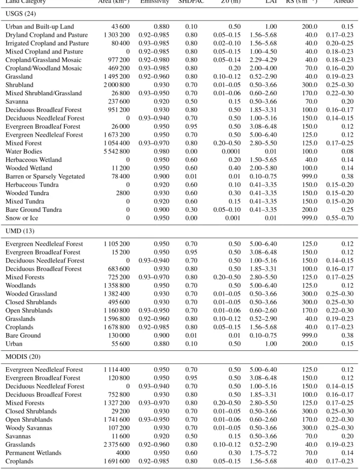
Table 2 summarizes the land areas and key parameters of each LULC dataset that are employed in the Noah LSM.
Each land cover class is associated with a particular pa-rameter value as governed by lookup tables in Noah. These parameters are crucial to the balances of land–vegetation– atmosphere energy, momentum, and water. For example, land surface emissivity and albedo are important for deter-mining L–A energy exchange (Eqs. 2 through 4), while SHD-FAC, LAI, and RS are keys to estimate ET. Working to-gether, these LSM parameters contribute to the solving of the land surface energy and water balance in the model, which subsequently are coupled to and impact upon important at-mospheric processes – e.g., temperature, wind, cloud, and boundary layer structure, as well as atmospheric chemistry and air quality.
2.4 Model evaluation
The results of the NU-WRF simulations were compared to the available observations from both ground and space plat-forms. The measurements of two meteorological parameters, air temperature at 2 m (T2) and water vapor content at 2 m (Q2), were obtained from the NCEP ADP Global Upper Air and Surface Weather Observations database (ADP: http://rda. ucar.edu/datasets/ds337.0/). The measurements of two sur-face air quality components, O3and particulate matter with aerodynamic diameter less than 2.5 µm (PM2.5), were
ob-tained from the Air Quality System (AQS) mainob-tained by the USEPA (http://www.epa.gov/ttn/airs/airsaqs/). The aerosol optical depth (AOD) observations at various wavelengths were obtained either from the ground based Aerosol Robotic Network (AERONET, http://aeronet.gsfc.nasa.gov/) or from the MODIS sensors on board the satellites Terra and Aqua, as well as the Multi-angle Imaging Spectroradiometer (MISR) sensor onboard Terra (http://disc.sci.gsfc.nasa.gov/giovanni/ overview/index.html). Three statistical measures were com-puted for the model evaluation. They are the normalized bias (NB), normalized gross error (NGE), and correlation coeffi-cient (Rvalue).
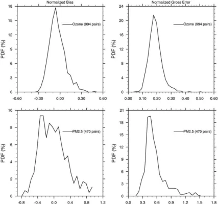
Fig. 2.Probability distributions of NB and NGE from individual site for the E USGS.
have NGE smaller than 50 %. When examining the model results integrated through the entire vertical layers (column AOD), NU-WRF commonly underestimates aerosols in com-parison with the AERONET and satellite measurements. It compares better to the AERONET AODs but noticeably worse to both the MODIS and MISR observations. Both the E UMD and E MODIS yield the similar statistics for the model/observation comparison when averaged over the en-tire CONUS domain (Table 3). If only urban grids are se-lected for comparison, however, the E MODIS gives the least biases for both ozone (2.4 % NB vs. more than 5 % from the E USGS and E UMD) and PM2.5(7.7 % NB vs. 26.1 % for the E USGS and 16.9 % for the E UMD).
3 Results and discussion
In order to quantify the impacts of LULC data on the com-plex interactions of the coupled L–A system, the results are broken down according to the “process chain” of Santanello et al. (2011). This enables the causal effects of different land cover types and associated parameters to be distinguished as the effects are felt into the atmosphere and chemistry com-ponents of the model.
3.1 Soil moisture (SM) and soil temperature (ST)
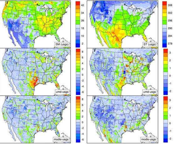
Figure 3 (top panels) shows the spatial distributions of 5-day average SM and ST over the CONUS domain from the
E USGS. In general, the soil is wet in eastern US and dry in the southwest region (left top panel). Over 0.3 m3m−3 val-ues are common in the Midwest and the Great Plains, where the dominant LULC is cropland or cropland/natural land mo-saic. High SM is also found along the North Pacific coast ar-eas and northern Montana. On the other hand, low SM (less than 0.06 m3m−3)is seen in southeastern California and the central boarder areas of Arizona and Utah, whose LULC is barren land or shrubland. The average SM spatial pattern fol-lows closely to that of the initial SM from the 3.5 yr spin-up simulation of the offline LIS, implying a long soil memory that warrants an extended LIS spin-up to allow reaching equi-librium.
Table 2.Land cover classification and its associated key parameter values.
Land Category Area (km2) Emissivity SHDFAC Z0 (m) LAI RS (s m−1) Albedo USGS (24)
Urban and Built-up Land 43 600 0.880 0.10 0.50 1.00 200.0 0.15 Dryland Cropland and Pasture 1 303 200 0.92–0.985 0.80 0.05–0.15 1.56–5.68 40.0 0.17–0.23 Irrigated Cropland and Pasture 80 400 0.93–0.985 0.80 0.02–0.10 1.56–5.68 40.0 0.20–0.25 Mixed Cropland and Pasture 0 0.92–0.985 0.80 0.05–0.15 1.00–4.50 40.0 0.18–0.23 Cropland/Grassland Mosaic 977 200 0.92–0.980 0.80 0.05–0.14 2.29–4.29 40.0 0.18–0.23 Cropland/Woodland Mosaic 469 200 0.93–0.985 0.80 0.20 2.00–4.00 70.0 0.16–0.20 Grassland 1 495 200 0.92–0.960 0.80 0.10–0.12 0.52–2.90 40.0 0.19–0.23 Shrubland 2 000 800 0.930 0.70 0.01–0.05 0.50–3.66 300.0 0.25–0.30 Mixed Shrubland/Grassland 26 800 0.93–0.950 0.70 0.01–0.06 0.60–2.60 170.0 0.22–0.30 Savanna 237 600 0.920 0.50 0.15 0.50–3.66 70.0 0.20 Deciduous Broadleaf Forest 951 200 0.930 0.80 0.50 1.85–3.31 100.0 0.16–0.17 Deciduous Needleleaf Forest 0 0.93–0.940 0.70 0.50 1.00–5.16 150.0 0.14–0.15 Evergreen Broadleaf Forest 26 000 0.950 0.95 0.50 3.08–6.48 150.0 0.12 Evergreen Needleleaf Forest 1 673 200 0.950 0.70 0.50 5.00–6.40 125.0 0.12 Mixed Forest 1 054 400 0.93–0.970 0.80 0.20–0.50 2.80–5.50 125.0 0.17–0.25 Water Bodies 5 542 800 0.980 0.00 0.0001 0.01 100.0 0.08 Herbaceous Wetland 0 0.950 0.60 0.20 1.50–5.65 40.0 0.14 Wooded Wetland 11 200 0.950 0.60 0.40 2.00–5.80 100.0 0.14 Barren or Sparsely Vegetated 78 400 0.900 0.01 0.01 0.10–0.75 999.0 0.38 Herbaceous Tundra 0 0.920 0.60 0.10 0.41–3.35 150.0 0.15–0.20 Wooded Tundra 2800 0.930 0.60 0.30 0.41–3.35 150.0 0.15–0.20 Mixed Tundra 0 0.920 0.60 0.15 0.41–3.35 150.0 0.15–0.20 Bare Ground Tundra 0 0.900 0.30 0.05–0.10 0.41–3.35 200.0 0.25 Snow or Ice 0 0.950 0.00 0.001 0.01 999.0 0.55–0.70
UMD (13)
Evergreen Needleleaf Forest 1 105 200 0.950 0.70 0.50 5.00–6.40 125.0 0.12 Evergreen Broadleaf Forest 15 200 0.950 0.95 0.50 3.08–6.48 150.0 0.12 Deciduous Needleleaf Forest 0 0.93–0.940 0.70 0.50 1.00–5.16 150.0 0.14–0.15 Deciduous Broadleaf Forest 683 600 0.930 0.80 0.50 1.85–3.31 100.0 0.16–0.17 Mixed Forests 725 200 0.93–0.970 0.80 0.20–0.50 2.80–5.50 125.0 0.17–0.25 Woodlands 1 358 800 0.950 0.70 0.50 5.00–6.40 125.0 0.12 Wooded Grassland 1 382 400 0.930 0.70 0.01–0.05 0.50–3.66 300.0 0.25–0.30 Closed Shrublands 495 600 0.930 0.70 0.01–0.05 0.50–3.66 300.0 0.25–0.30 Open Shrublands 1 160 800 0.93–0.950 0.70 0.01–0.06 0.60–2.60 170.0 0.22–0.30 Grasslands 1 596 800 0.92–0.960 0.80 0.10–0.12 0.52–2.90 40.0 0.19–0.23 Croplands 1 678 800 0.92–0.985 0.80 0.05–0.15 1.56–5.68 40.0 0.17–0.23 Bare Ground 130 000 0.900 0.01 0.01 0.10–0.75 999.0 0.38
Urban 55 600 0.880 0.10 0.50 1.00 200.0 0.15
MODIS (20)
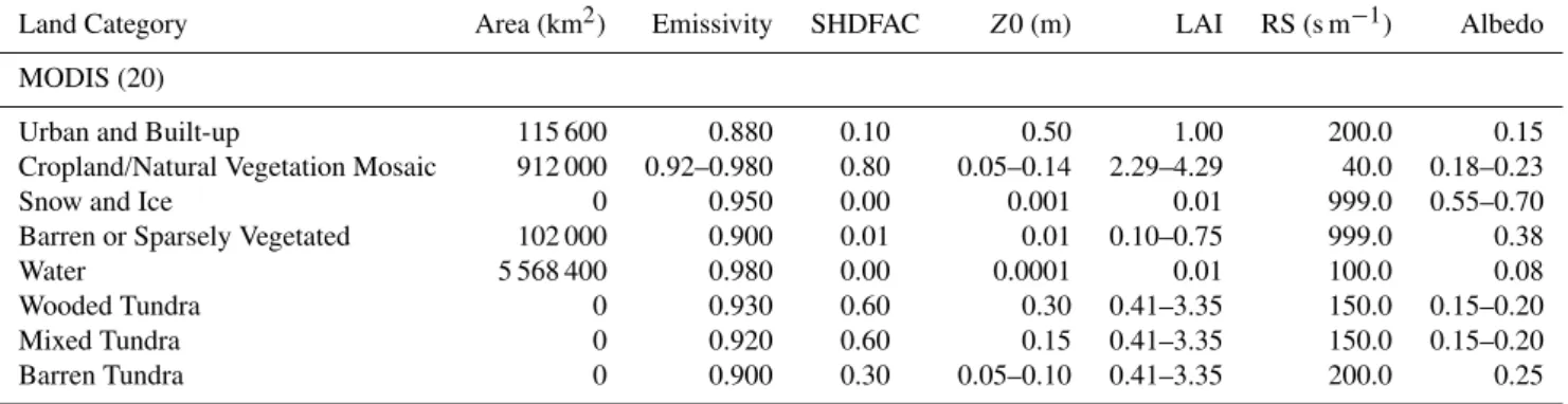
Table 2.Continued.
Land Category Area (km2) Emissivity SHDFAC Z0 (m) LAI RS (s m−1) Albedo MODIS (20)
Urban and Built-up 115 600 0.880 0.10 0.50 1.00 200.0 0.15 Cropland/Natural Vegetation Mosaic 912 000 0.92–0.980 0.80 0.05–0.14 2.29–4.29 40.0 0.18–0.23 Snow and Ice 0 0.950 0.00 0.001 0.01 999.0 0.55–0.70 Barren or Sparsely Vegetated 102 000 0.900 0.01 0.01 0.10–0.75 999.0 0.38 Water 5 568 400 0.980 0.00 0.0001 0.01 100.0 0.08 Wooded Tundra 0 0.930 0.60 0.30 0.41–3.35 150.0 0.15–0.20 Mixed Tundra 0 0.920 0.60 0.15 0.41–3.35 150.0 0.15–0.20 Barren Tundra 0 0.900 0.30 0.05–0.10 0.41–3.35 200.0 0.25
Table 3.Summary of statistics comparing with observations.
Data Source T2 Q2 O3 PM2.5 550 nm 555 nm 380 nm 500 nm 675 nm 870 nm
ADP ADP AQS AQS MODIS MISR AOD from AERONET
# of pairs 177 022 153 350 73 267 52 895 3718 2897 110 112 115 132
E USGS
NB (%) −0.37 0.10 −5.10 3.77 −26.6 −55.4 −29.4 −24.9 −11.7 −16.4 NGE (%) 0.89 14.1 18.8 57.1 86.3 59.8 43.2 40.1 40.5 41.7
Rvalue 0.86 0.87 0.62 0.35 0.20 0.23 0.46 0.53 0.49 0.43
E MODIS
NB (%) −0.33 0.05 −4.51 2.68 −26.6 −55.6 −30.2 −25.5 −12.4 −16.9 NGE (%) 0.88 14.3 18.8 56.9 86.3 59.8 42.6 39.4 39.9 41.4
Rvalue 0.86 0.86 0.61 0.35 0.20 0.24 0.48 0.55 0.50 0.43
E UMD
NB (%) −0.25 0.00 −3.89 2.98 −26.6 −55.5 −30.9 −26.0 −13.1 −17.4 NGE (%) 0.88 14.0 18.7 57.1 86.0 59.8 43.0 40.1 40.4 41.7
Rvalue 0.86 0.86 0.62 0.34 0.20 0.23 0.47 0.53 0.49 0.42
NB=sim-obsobs ×100 %; NGE=|sim-obsobs |×100 %;Rvalue=correlation coefficient.
3 K higher soil temperature (right bottom panel) found in ur-ban LULC of E MODIS than that found in the same loca-tions of E USGS where the LULC is cropland. The differ-ences ofalbedoandemissivityin various LULC also explain the changes in ST found between the E UMD and E USGS (right middle panel).
Averaged over the land of the CONUS domain, the av-erage SM and ST are 0.2289 m3m−3 and 291.22 K, re-spectively, from the E USGS. After receiving 1.98 % (i.e., 0.25 mm grid−1, or approximately 2.61 km3 water over the domain’s land) more precipitation, E UMD’s SM is 1.92 % more than that based on the E USGS. Although it pro-duces 0.38 % (i.e., 0.05 mm grid−1) more precipitation, the E MODIS gives an almost same average SM as that from the E USGS. Compared with the average ST from the E USGS, E UMD models approximately 0.22 K higher ST, while E MODIS estimates around 0.02 K lower ST.
3.2 Latent heat flux (LH) and sensible heat flux (HFX)
Fig. 3.Spatial distribution of top soil moisture (SM, %, left panels) and average top soil temperature (ST, K, right panels) simulated using the USGS LULC and their differences with the results using the UMD (umd-usgs) and MODIS (modis-usgs) LULC.
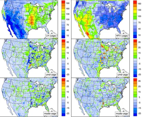
designated in the Great Plains have much smaller RS than the evergreen needleleaf forest in the North Pacific coast ar-eas (40 vs. 125 s m−1, Table 2), which leads to the higher ET and the subsequent higher LH in the Great Plains. Contrary to LH, high HFX is typically seen over the dry soil (Fig. 4, right panels). The high HFX found in the dry soil agrees with the study by Bindlish et al. (2001), who used the microwave remote sensing data to model the linkage between SM and HFX. The dry southwestern US typically sees an HFX more than 130 W m−2, while the wet eastern US experiences a less than 40 W m−2of HFX. The major metropolitan areas gen-erally experience higher HFX than the surrounding areas fol-lowing the land–air temperature gradient, exactly the oppo-site spatial pattern of that of LH. Taking the E USGS as an example and defining the surrounding areas as one grid ex-tension of each direction of an urban grid, the average ur-ban LULC sees an approximately 93 % higher HFX but 68 % lower LH.
Compared to the E USGS, the E UMD generates 15 to 25 W m−2 lower LH in the Central Valley areas of Califor-nia, the corridor areas extending from eastern Kansas, cen-tral Oklahoma, to northern Texas, and the sporadic areas in the eastern US. On the other hand, the E UMD generates up to 35 W m−2more LH in the limited area of
northeast-ern Texas and the sporadic areas of the eastnortheast-ern US. This can all be traced back to the different LULC assignments in USGS and UMD, as well as the resulting precipitation con-trast found in the E USGS and E UMD. For example, USGS designates the LULC in the aforementioned corridor areas as grassland/mixed forest (RS=125 s m−1) but UMD denotes it as closed shrubland (RS=300 s m−1). Obviously with the similar precipitation, closed shrubland tends to retain water better and then causes the lower QFX and LH. Meanwhile, although the limited areas of northeastern Texas is designated as cropland and evergreen needleleaf forest in USGS as op-posed to closed shrubland in UMD, it receives at least 20 mm more rainfall, which leads to the higher QFX and LH found in the E UMD. Again, the large urban (RS=200 s m−1) ex-pansion shown in MODIS explains the lower QFX an LH simulated over the major metropolitan areas in comparison to that from the E USGS. The domain-wide average QFX and LH for land are approximately 107 g m−2h and 74 W m−2, respectively, from the E USGS. The discrepancies among the results from the E USGS, E UMD, and E MODIS are all within 0.3 %.
Fig. 4.Same as Fig. 3 except for average latent heat flux (LH, W m−2, left panels) and sensible heat flux (HFX, W m−2, right panels).
occurring in the scattering regions in the Midwest and the Great Plains. The detailed LULC investigation reveals that the LULC changes with the large RS contrast give the big dif-ferences in temperature gradient and HFX. The areas with the largest HFX increases are usually designated as the closed shrubland in UMD while as the cropland or grassland in USGS. The largest HFX decreases occur where the LULC is forest or shrubland mixture in USGS and grassland or crop-land in UMD. On average, the E MODIS (Fig. 4, right bot-tom panel) generates around 1 % lower HFX over the land than the E USGS. However, the expanded urban areas found in MODIS do see a higher HFX and temperature gradient. The observation that large RS contrast results in big HFX change holds for this instance as well.
3.3 Air temperature at 2 m (T2) and water vapor content at 2 m (Q2)
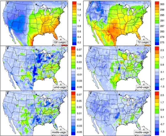
The land surface energy and water budgets reflected in QFX, LH, and HFX would impact the near-surface air temperature and moisture as illustrated in Fig. 5. The left panels display the spatial distributions ofQ2. Similar to SM, the eastern US generally finds a highQ2 (more than 0.01 kg kg−1) and the southwestern US sees less than 0.004 kg kg−1Q2. However, the northwestern US, where the high SM comparable with the eastern US is modeled, sees about half ofQ2 as that of the
eastern US, which follows that of QFX, reflecting that some LULCs retain soil water better than the others. In comparison to the E USGS, the E UMD simulates lowerQ2 in the large portions of the Midwest and the Great Plains but higherQ2 in the sporadic areas of the eastern US. The spatial pattern of the lowerQ2 appears to correspond to the lower LH (Fig. 4, left middle panel) but the spatial distribution of the higher
Q2 seems more of the effect of boundary layer structure – shallow PBLH implies less entrainment of dry and warm air into the PBL from the free atmosphere, thus a higherQ2. The urban and built-up land tends to have lowerQ2, as can be seen in Fig. 5, left bottom panel. In the region where it is designated as urban and built-up land in MODIS but not in USGS,Q2 is around 3 % higher from the E USGS than from the E MODIS.
Fig. 5.Same as Fig. 3 except for average water vapor content (Q2, %, left panels) and air temperature (T2, K, right panels) at 2 m.
the one of HFX sinceT2 is determined with HFX and sur-face skin temperature (e.g., Miglietta et al., 2009). The wet eastern US has a small temperature gradient (less than 0.2 K for the vast areas), while the dry southwestern region expe-riences a high (typically more than 4 K) temperature gradi-ent. Following the case of HFX, the average urban LULC sees an approximately 1 K warmer T2 than the surround-ing areas. The LULC-difference-induced temperature change would influence biogenic emissions and thermal chemical reaction processes that consequently would alter the atmo-spheric composition and air quality.
3.4 Wind speed and planetary boundary layer height (PBLH)
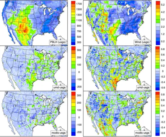
The LH, HFX, and QFX calculated from the land surface model provide the lower boundary conditions for the verti-cal transport simulation, and thus impact the PBL structure and its evolution, as reflected in PBLH. Figure 6 (left pan-els) displays the average PBLH spatial distribution from the E USGS (left top panel) and its comparisons with the results from the E UMD (left middle panel) and E MODIS (left bot-tom panel). It can be found that the PBLH distribution ap-pears similar to the HFX distribution. This agrees with the physical basis for PBL growth being primarily driven by the buoyancy fueled by surface heating, and was confirmed by
observations obtained from the AMMA campaign (Kohler et al., 2010). The high PBLH is found in the dry southwest-ern US, with the maximum (more than 1700 m) being in western Texas and central New Mexico and the minimum (less than 400 m) in eastern Mississippi and central Alabama. The daytime PBLH map closely mimics the daily average map with the maximum PBLH exceeding 4000 m in western Texas. During nighttime, however, the highest PBLH (up to 700 m) is found in the Great Plains. It is worth noting that during daytime the average PBLH over the urban areas (ap-proximately 1400 m) is about 14 % higher than that of the surrounding areas, while at night the average PBLH over the urban areas is about 10 m smaller than that over the surround-ing areas. The daily average urban PBLH (around 620 m) is approximately 11 % more than the PBLH of the surrounding areas.
Fig. 6.Same as Fig. 3 except for average PBL height (PBLH, m, left panels) and surface wind speed (m s−1, right panels).
the vertical mixing of heat, moisture, momentum, and mass, and have a profound effect on air quality. In addition, deeper PBLH growth implies larger entrainment of dry and warm air into the PBL from the free atmosphere. This feedback then favors a warmer, drier PBL as reflected in the resultantT2 andQ2 conditions with implications for atmospheric chem-istry.
Figure 6 (right panels) illustrates the surface wind speed that is directly affected by the LULC through friction and, to a lesser extent, through the LULC impacts on heat fluxes as demonstrated in the previous sections. As compared to the E USGS, the E UMD and E MODIS generate slightly higher average surface wind (1.98 m s−1and 1.99 m s−1vs. 1.97 m s−1, respectively) for the land with the largest changes (approximately 1 m s−1) occurring in southern Texas, the central Florida, and the scattered areas across the rest of the US (right middle panel), as well as the noticeable decrease (up to 0.6 m s−1) in south Wyoming and the scattered ar-eas of the other parts of the US (right bottom panel). The LULC examination reveals that, in general, the wind speed increases when the LULC with large Z0 in USGS is re-placed with the LULC with smallZ0 in the other datasets, and vice verse. For example, the LULC in southern Texas is designated as cropland or cropland/natural land mosaic (Z0=0.05–0.20 m) in USGS. When it is replaced with the
closed shrubland (Z0=0.01–0.05 m) in UMD, the average wind speed increases by 0.6–1.0 m s−1. On the other hand, when the LULC in south Wyoming designated as the shrub-land or shrubshrub-land mixture in USGS is replaced with the grassland (Z0=0.10–0.12 m) in MODIS, the average wind speed decreases by 0.6 m s−1. The changed surface wind impacts soil erosion and dust emissions, as well as affects the horizontal movements of mass and energy, which subse-quently impact air quality, as will be discussed in the follow-ing sections.
3.5 Emissions of dust and biogenic volatile organic compound (BVOC)
Fig. 7.Same as Fig. 3 except for average dust emissions (kg km−2h, left panels) and biogenic isoprene emissions (mol km−2h, right panels).
southeastern California. The noticeable dust emissions are also found over the Sonoran Desert located in southern Cali-fornia, southwestern Arizona, and northwestern Mexico, as well as over the Chihuahuan Desert in southern Arizona and New Mexico, southwestern Texas, and northern Mex-ico. The average daily dust emissions over the CONUS are 37 735, 39 221, and 39 105 metric tons from the E USGS, E UMD, and E MODIS, respectively, which are comparable with the April average dust load (40 500 metric tons day−1) over North America estimated by Park et al. (2010) using their newly developed windblown dust module. The SM role in the change in dust emissions due to the LULC data selec-tion is negligible and the increase/decrease in emissions is almost all attributed to the wind speed difference induced by the different LULC data usage.
Biogenic emissions depend on the LULC and the sur-rounding environment (Guenther et al., 2006). In this study, the LULC data used in the biogenic emissions module, MEGAN2, are based on both AVHRR and MODIS that are different from either LULC used in the experiments. There-fore, the discussion on the impact of the LULC data on BVOC emissions is limited to the indirect effects through the emissions adjustment by the ambient temperature and solar radiation that would be altered by the LULC change, as dis-cussed in the previous sections. Figure 7 (right panels)
illus-trates the spatial distribution of the average biogenic isoprene emissions from the E USGS and its contrast maps in compar-ison with the E UMD and E MODIS. Large isoprene emis-sions are observed in the eastern US with the peak (more than 35 mol km−2h) occurring in the Ozarks (covering southern Missouri and northern Arkansas) and eastern Texas/western Louisiana. This spatial distribution matches the results by Xu et al. (2002), who employed the AVHRR data and the Biogenic Emission Inventory System (BEIS) model to esti-mate the isoprene emissions for the eastern US, and by Tao et al. (2003), who also employed BEIS. The isoprene emissions contrast maps (right middle and bottom panels) closely fol-low the spatial distributions of the surface temperature con-trasts (Fig. 5, right panels). The difference can reach more than 6 mol km−2h. Over the CONUS domain, the daily av-erage isoprene emissions are approximately 88 752 metric tons based on the E USGS. The results from the E UMD and E MODIS are 3.1 % and 1.5 % higher than that of the E USGS, respectively, and are largely a function of higher
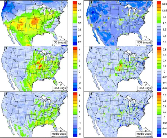
Fig. 8.Same as Fig. 3 except for average surface ozone concentration (ppbv, left panels) and NO2concentration (ppbv, right panels).
3.6 Air quality
The LULC change induces changes in meteorological fields, e.g., the temperature, wind, and PBLH, as well as in emis-sions, which results in a profound impact on air quality. High temperature generally favors ozone formation. Strong wind moves the pollutants fast and further away. Deep PBL is good for pollutant vertical mixing. Emissions directly enter the at-mospheric pollutants mass balance. Three pollutants – ozone, nitrogen dioxide (NO2), and PM2.5 – are used as proxy to discuss the LULC impact on air quality. Ozone is a criterion pollutant regulated by the USEPA. As a secondary pollutant (i.e., not directly emitted from a source), ozone forms in the presence of its precursors under the favorable meteorologi-cal conditions, e.g., stagnant high-pressure system featuring strong solar radiation and high air temperature (e.g., Seinfeld and Pandis, 2006). NO2, on the other hand, is a primary pol-lutant that is emitted from a large pool of anthropogenic and natural sources. It is also regulated by the USEPA and is one of the two (the other is VOC) key precursors of ozone.
Figure 8 displays the spatial distributions of average sur-face ozone concentration (left panels) and NO2 (right pan-els) from the E USGS and their contrast maps to the results from the E UMD and E MODIS. As a primary pollutant, NO2distributes heterogeneously in space with high concen-trations centering in the major metropolitan regions and the
Ohio River Valley, where large emissions sources are identi-fied. The urban grids observe, on average, more than twofold of surface NO2 than the surrounding areas (14.2 ppbv vs. 6.7 ppbv). On the other hand, the secondary ozone experi-ences a relatively homogenously spatial distribution. Rela-tively high ozone (more than 45 ppbv) is seen in the south-ern Great Plains and southsouth-ern California. The difference be-tween urban and the surrounding areas is small with the ur-ban grids observing less than 2 ppbv of surface ozone than the surrounding grids.
deposition represent the major NO2removal mechanism in the atmosphere (e.g., Seinfeld and Pandis, 2006). The dry deposition velocity of HNO3 (figure not shown) is lower in those regions reducing the NO2removal from the atmo-sphere. The aforementioned reasons also explain what hap-pens in the metropolitan areas. In the regions where all three datasets designate the LULC as urban and built-up land, the E UMD and E MODIS observe the respective 0.25 ppbv and 0.78 ppbv lower NO2 concentrations averaged over the ur-ban grids as compared to the results from the E USGS. The averaged HNO3dry deposition velocity and surface temper-ature from the E UMD and E MODIS are approximately 0.2 cm s−1 larger and 0.5 K higher, respectively, than from the E USGS favoring the reduced NO2. The largely en-hanced PBLH from the E UMD (around 35 m deeper) and E MODIS further dilutes NO2as compared to that from the E USGS.
In the rural areas where ozone formation is almost always limited to the availability of NOx (i.e., NO2 + NO), mete-orology can largely explain the difference among each ex-periment. For example, up to 4 ppbv more ozone is observed in the stretched areas of the Midwest from the E UMD than from the E USGS (Fig. 8, left middle panel). HigherT2 sim-ulated in those areas is one of the key drivers for this obser-vation – higher temperature not only increases soil NO emis-sions (e.g., Williams et al., 1992; Tao et al., 2003) that fuel ozone formation there but also favors the thermodynamics of ozone generation. The replacement of cropland designated in USGS with forest/closed shrubland in UMD results in the re-duced ozone dry deposition velocity for the aforementioned areas, thus the increased ozone concentration. The smaller ozone dry deposition velocity found in forest than in crop-land is consistent with the results from a model study by Miao et al. (2006). The deeper PBLH from the E UMD in those areas (Fig. 6, left panels) reduces surface ozone con-centration but not enough to totally offset the ozone increase due to the changes in temperature and dry deposition. More-over, as discussed in Sect. 3.4, deeper PBLH tends to entrain more warm and dry air from the free troposphere that may favor ozone generation. The net PBLH effect on ozone air quality therefore highly depends on the competition of ver-tical mixing and photochemical formation. In the urban ar-eas, however, where either NOxor VOC can limit ozone for-mation, the explanation is not that straightforward. As dis-cussed in the NO2comparison, the PBLH and surface tem-perature from the E MODIS are both higher than from the E USGS. The effects of these two factors on ozone forma-tion are potentially opposite. In addiforma-tion, in the NOx-limited regime the deep PBLH-induced surface NOxdecrease would further suppress ozone formation, while in the VOC-limited regime the reduced NOx tends to produce more ozone due to the reduced NOxtitration effect (e.g., Seinfeld and Pandis, 2006). Together these effects cause a moderate average ozone differences (within 0.5 ppbv) over the urban grids among the three experiments.
From the air quality regulation perspective, it is also in-teresting to know how the LULC impacts the frequency of high ozone occurrences. It is found that there are 467 occurrences of surface 8 h-average ozone concentration ex-ceeding 75 ppbv, the National Ambient Air Quality Standard for ozone set by the USEPA (http://www.epa.gov/air/criteria. html), from the E USGS. The E UMD and E MODIS gener-ate 32 % and 3 % more high ozone occurrences, respectively. PM2.5 is another criterion pollutant and can be both pri-mary and secondary origin. The spatial distributions (figures not shown) of average surface PM2.5from the E USGS and its difference with the E UMD and E MODIS are similar to those of NO2(Fig. 8, right panels), with more than 10 µg m−3 being common in major metropolitan areas and the Mid-west. The main difference between spatial distributions of NO2and PM2.5is that very high concentrations (greater than 35 µg m−3) are found in southern California, southwestern Arizona, and northwestern Mexico, where the wind-blown dust emissions dominate. The smaller PBLH and less rainfall (thus less wet removal) found in the Missouri/Kansas border and northeastern Oklahoma from the E UMD as compared to that from the E USGS largely explains the higher PM2.5 (up to 4 µg m−3) in those regions based on the E UMD. Sim-ilarly, the larger PBLH in the urban areas simulated from the E MODIS contributes the reduced PM2.5there.
3.7 Implication of urbanization effect on ozone air quality
According to the 2010 US census, approximately 80.7 % of the population lives in urban areas (http://www.census.gov/ geo/www/ua/2010urbanruralclass.html). The highly popu-lated urban areas present a distinct local climate featuring some unique phenomenon such as urban heat islands as a re-sult of complex interactions between humans and nature – e.g., changes in short/long-wave solar radiation due to large emissions (albedoandemissivity), changes in airflow due to increased friction (Z0), and reduced ET due to vegetation removal (RS) (e.g., Coutts et al., 2007). The subsequent im-pacts on air quality and human health can be large and need to be investigated.
Table 4.Comparison of key parameters associated with urban ozone air quality over the MODIS urban areas.
USGS Land Category Area (km2) SM (%) T2 (K) Wind (m s−1) PBLH (m) O3Dry Dep. (cm s−1)
usgs modis usgs modis usgs modis usgs modis usgs modis
Urban and Built-up Land 42 400 31.5 32.7 294.4 295.2 1.55 1.51 626 686 0.27 0.28 Dryland Cropland and Pasture 14 000 24.4 32.0 297.8 299.6 1.55 1.62 694 913 0.51 0.53 Cropland/Grassland Mosaic 6800 28.3 33.0 295.0 296.6 1.40 1.33 668 837 0.57 0.59 Cropland/Woodland Mosaic 8800 28.4 31.9 294.9 296.3 1.21 1.28 509 659 0.46 0.46 Grassland 8000 23.5 31.3 296.2 297.4 2.28 1.89 997 1110 0.43 0.46 Shrubland 5200 14.6 24.5 294.2 295.5 1.99 1.72 822 852 0.34 0.43 Mixed Shrubland/Grassland 2400 24.4 24.0 291.1 291.7 1.38 1.48 412 428 0.37 0.40 Savanna 3600 29.8 31.8 291.5 291.8 2.48 2.49 505 518 0.41 0.41 Deciduous Broadleaf Forest 9600 28.2 29.7 292.7 293.6 1.63 1.63 548 615 0.51 0.51 Evergreen Needleleaf Forest 8800 27.2 32.3 293.9 295.5 1.35 1.33 594 753 0.48 0.52 Mixed Forest 1200 29.1 32.6 294.1 295.6 1.53 1.78 560 712 0.45 0.45 Water Bodies 4000 – 12.2 292.2 292.5 2.98 3.01 294 352 0.21 0.21 Wooded Wetland 800 30.6 34.5 300.0 301.1 1.90 2.10 730 867 0.40 0.41 Areal Weighted Average – 28.0 31.6 294.6 295.7 1.65 1.61 634 736 0.39 0.40
designated as urban by both MODIS and USGS, the gradi-ents are the major driving force of the modeled differences since the land characteristics are the same for the same land categories from the different LULC datasets (see Table 2). Over the areas designated as urban by MODIS but defined as non-urban by USGS, however, both local effects (through different land characteristics, e.g.,roughness,albedo, LAI, and RS) and gradients play roles in modeled discrepancies between the E USGS and E MODIS.
Table 4 summarizes the averages of some parameters key to ozone air pollution. It can be found that only 36.7 % of the MODIS urban is designated as urban and built-up land in USGS, with various croplands (25.6 %), various forests (17.0 %), grassland (6.9 %), and shrubland (4.5 %) rounding up to the top five LULC in USGS for the MODIS urban. As a result, the SM increases by 13 % over the MODIS urban areas as compared to the same regions from the E USGS with the large SM change (greater than 30 %) occurring where shrubland, dryland cropland/pasture, or grassland is converted into urban area. On average,T2 increases by 1.1 K based on the E MODIS, with the large increases observed where urban area sprawls into cropland or forest. PBLH ex-periences the increase across all the USGS LULCs that are designated as urban by MODIS, with the largest enhance-ment (219 m) happening in the places that used to be dryland cropland/pasture. Surface wind speed changes in both direc-tions. While converting grassland and shrubland into urban tends to decrease it, urban sprawling into mixed forest or wooded wetland is likely to increase wind speed. On aver-age, surface wind speed displays a small decrease (less than 3 %) during the urbanization. Ozone dry deposition velocity undergoes a moderate change (less than 5 %) as well with the largest increase (approximately 26 %) occurring in the places where shrubland in USGS changes to urban in MODIS.
Fig. 9.Probability distributions of surface 8 h-average ozone for the E USGS and E MODIS.
(i.e., more than 75 ppbv) appears reduced from 79 ppbv in the E USGS to 77 ppbv in the E MODIS. It should be noted that the anthropogenic emissions change due to urbanization has not been taken into account in this study. Depending on the urban emissions characteristics (e.g., NOxsensitive or VOC sensitive), such change can complicate the urban ozone is-sues.
4 Summary and conclusion
Three commonly used LULC datasets – i.e., USGS, UMD, and MODIS – have been applied to the newly developed NU-WRF system to investigate the land cover effects on atmo-spheric processes and air quality over the CONUS domain. These three datasets display large differences in land cover classifications and assignments, where the overall agree-ments of MODIS/USGS, MODIS/UMD, and USGS/UMD are 55.8 %, 53.7 %, and 47.8 %, respectively, when the eight common land classifications employed in all three datasets are considered. There are two major model procedures for this study. The three LULC datasets are first plugged in the offline LIS system for spin-up to achieve the soil equilibrium state, and the results from the offline LIS then provide the surface boundary and initial conditions to the NU-WRF. The NU-WRF results are compared with the available observa-tions and the results show NU-WRF does a reasonably good simulation of physical, chemical, and biological processes.
The offline LIS results show that large initial SM differ-ence (30–50 %) exists in the regions where woodland/closed shrubland changes to cropland or cropland is cleared for ur-ban areas. The initial SM difference carries over into the NU-WRF simulation to be reflected in the similar spatial pattern of the average SM distribution. It also results in a notice-able precipitation change – in comparison to the E USGS, the E UMD and E MODIS produce 0.25 mm grid−1 and 0.05 mm grid−1more rainfall averaged over the domain land. LH and HFX distributions are closely coupled to the SM as well. Wet soil generally leads to high LH and low HFX, while dry soil does the opposite. When land with small RS changes to the one with large RS (e.g., cropland/grassland to shrub-land/urban area), LH tends to decrease and HFX appears to increase. This is because RS is one key to estimate ET that is important to both water and energy cycles between the land and the atmosphere. Large RS restricts ET and allows more energy into HFX. The energy change due to land cover change at the land surface would propagate into the overlay-ing atmosphere and lead to changes in temperature, PBLH, and wind that are important to the atmospheric composition evolution and air quality. For example, regions with high HFX tend to have high surface temperature and deep PBLH. Therefore, change in LULC from the one favoring large ET to the one with small ET would increase surface temperature and enhance PBLH. This is what happens when cropland is converted into urban land, where the averageT2 increases by
approximately 1 K and the PBLH is around 11 % larger. Land with largeZ0 tends to have reduced surface wind, as evi-denced by the 0.6–1.0 m s−1decreases in the average wind speed in southern Texas where the shrubland in UMD is con-verted into the cropland in USGS.
The LULC-change-induced meteorology change would subsequently affect land surface emissions and air qual-ity. SM and surface wind directly determine how much dust is produced and enters into the atmosphere. This study shows that it is mainly wind that dictates the dust emission changes due to the selections of different LULC datasets. Domain-wide, the E UMD and E MODIS respectively pro-duce 3.9 % and 3.6 % more dust than the E UDSG. Bio-genic emissions are affected as well. As compared to the E USGS, the E UMD and E MODIS respectively generate 3.1 % and 1.5 % more isoprene, and 2.7 % and 0.8 % more terpenes. Air quality responds to the meteorology and emis-sions changes in a complex way. The surface concentration of the primary pollutant NO2 tends to decrease where the deep PBL develops, such as the case of converting USGS’s cropland/grassland into MODIS’s urban area. The enhanced dry deposition of HNO3, a major NO2terminal species, over urban areas also contributes to the NO2reduction under the cropland-changed-to-urban scenario. The response of surface ozone, a secondary pollutant, to the LULC change is more complex. Although high temperature and weak wind mostly favor ozone formation, depending on the local emissions characteristics, surface ozone can be enhanced or suppressed in response to PBLH change, as evidenced under the same cropland-changed-to-urban scenario. For the simulation pe-riod, the E UMD models noticeably more high ozone that exceeds the US surface ozone standard and the E MODIS yields a relatively smaller increase in ozone standard viola-tions as compared to the E USGS.
The impact of urbanization on air quality is investigated in the context of the conceptual land cover change found in USGS and MODIS. MODIS carries greater than 100 % more urban coverage than USGS. The virtual urban expan-sion in MODIS produces higher SM, lower LH, higher HFX, higher surface temperature, weaker wind, and deeper PBLH. As a result, surface NO2 tends to reduce, whereas surface ozone can change in both directions due to the compensating feedbacks. Overall, urbanization appears to cause less low ozone (smaller than 30 ppbv) but more high ozone (greater than 70 ppbv) occurrences.
intended, this study is able to isolate the impact of secondary (via meteorology) effects of land and atmosphere feedbacks on emissions and chemistry. Second, although it provides some insights into the consequences of LULC changes on at-mospheric processes and air quality, this study employs three datasets derived from the different satellite sensors and clas-sification methods that make the land definition inconsistent across the datasets. In the future, application of time series LULC data derived from the same sensor and same classi-fication method will greatly improve the understanding of the impacts of LULC change on air quality, especially over the populated urban areas. The forthcoming MODIS 2010 data that will be ready for NU-WRF application (vs. MODIS 2002 as used in this study) will provide a good opportunity to do such investigation. Last but not the least, the model internal variability, which arises from the nonlinear nature of atmospheric processes such that the model is sensitive to perturbations of initial conditions (ICs) (e.g., Giorgi and Bi, 2000; Vanvyve et al., 2008), is not explored in this study. Changes in atmospheric parameters due to physical modifi-cations of a model are only significant when outside of the model internal variability. Based on the study by Vanvyve et al. (2008), who investigated the regional model internal vari-ability by randomly altering the ICs, the maximum variabil-ity for 5-day-average air temperature at 10 m and boundary layer wind speed ranged from 0.03 to 0.18 K, and from 0.06 to 0.31 m s−1, respectively, depending on the location in their West African domain. Giorgi and Bi (2000) conducted the model internal variability study for the eastern China domain and concluded that the model response to perturbations was insensitive to the origin, location, and the magnitude of per-turbation but sensitive to the perper-turbation timing. The vari-ability for the daily average surface temperature, wind speed, and water vapor content over late May to early June was within 0.1 K, 0.1 m s−1, and 0.1 g kg−1, respectively. If those numbers are assumed to be the model random error bounds, it is obvious that the modeled differences (Fig. 5 and right panel of Fig. 6) due to the usage of different LULC datasets are well beyond the model internal variability.
In conclusion, this study has shown the importance of land cover data on offline and coupled L–A and chemistry predic-tion. There is inconsistency amongst ancillary dataset appli-cation in the Earth system models to date, and the uncertainty introduced as a result has gone largely ignored. With contin-ued advancements of satellite-based land cover datasets, it is therefore critical to make such assessments as were per-formed here.
Acknowledgements. The authors would like to thank the NASA Center for Climate Simulation (NCCS) for supercomputing and mass storage support. This research was partially funded by the NASA’s Modeling, Analysis, and Prediction (MAP) program and by the NASA’s Atmospheric Composition: Modeling and Analysis (ACMAP) program at the Goddard Space Flight Center of NASA.
Edited by: B. N. Duncan
References
Atkinson, R., Baulch, D. L., Cox, R. A., Crowley, J. N., Hamp-son, R. F., Hynes, R. G., Jenkin, M. E., Rossi, M. J., Troe, J., and IUPAC Subcommittee: Evaluated kinetic and photochemi-cal data for atmospheric chemistry: Volume II – gas phase re-actions of organic species, Atmos. Chem. Phys., 6, 3625–4055, doi:10.5194/acp-6-3625-2006, 2006.
Berge, E., Huang, H.-C., Chang, J., and Liu, T.-H.: A study of the importance of initial conditions for photochemical oxidant mod-eling, J. Geophys. Res., 106, 1347–1363, 2001.
Bindlish, R., Kustas, W. P., French, A. N., Diak, G. R., and Mecikalski, J. R.: Influence of near-surface soil moisture on re-gional scale heat fluxes: Model results using microwave remote sensing data from SGP97, IEEE T. Geosci. Remote Sens., 39, 1719–1728, 2001.
Case, J. L., Crosson, W. L., Kumar, S. V., Lapenta, W. M., and Peters-Lidard, C. D.: Impacts of High-Resolution Land Surface Initialization on Regional Sensible Weather Forecasts from the WRF model, J. Hydrometeorol., 9, 1249–1266, 2008.
Case, J. L., Kumar, S. V., Srikishen, J., and Jedlovec, G. J.: Improv-ing Numerical Weather Predictions of Summertime Precipitation over the Southeastern United States through a High-Resolution Initialization of the Surface State, Weather Forcast., 26, 785–807, 2011.
Charusombat, U., Niyogi, D., Kumar, A., Wang, X., Chen, F., Guen-ther, A., Turnipseed, A., and Alapaty, K.: Evaluating a new depo-sition velocity module in the Noah land-surface model, Bound.-Lay. Meteorol., 137, 271–290, 2010.
Chen, J., Avise J., Guenther, A., Wiedinmyer, C., Salathe, E., Jack-son, R. B., and Lamb, B.: Future land use and land cover in-fluences on regional biogenic emissions and air quality in the United States, Atmos. Envrion., 43, 5771–5780, 2009.
Cheng, F.-Y., Kim, S., and Byun, D.-W.: Application of high res-olution land use and land cover data for atmospheric modeling in the Houston-Galveston Metropolitan area: Part II. Air quality simulation results, Atmos. Environ., 42, 4853–4869, 2008. Chin, M., Ginoux, P., Kinne, S., Torres, O., Holben, B. N., Duncan,
B. N., Martin, R. V., Logan, J. A., Higurashi, A., and Nakajima, T.: Tropospheric aerosol optical thickness from the GOCART model and comparisons with satellite and Sun photometer mea-surements, J. Atmos. Sci., 59, 461–483, 2002.
Chou, M.-D. and Suarez, M. J.: A solar radiation parameteriza-tion (CLIRAD-SW) for atmospheric studies, NASA Tech. Rep. NASA/TM-1999-10460, Washington DC, Vol. 15, 38 pp., 1999. Coutts, A. M., Beringer, J., and Tapper, N. J.: Impact of increasing urban density on local climate: Spatial and temporal variations in the surface energy balance in Melbourne, Australia, J. Appl. Meteorol. Clim., 46, 477–493, 2007.
Danko, D. M.: The Digital Chart of the World, GeoInfo Systems, 2, 29–36, 1992.
Deardorff, J. W.: Efficient prediction of ground surface temperature and moisture with inclusion of a layer of vegetation, J. Geophys. Res., 83, 1889–1903, doi:10.1029/JC083iC04p01889, 1978. Ek, M. B., Mitchell, K. E., Lin, Y., Rogers, E., Grunmann, P.,
Environmental Prediction operational mesoscale Eta Model, J. Geophys. Res., 108, 8851, doi:10.1029/2002JD003296, 2003. Emmons, L. K., Walters, S., Hess, P. G., Lamarque, J.-F., Pfister,
G. G., Fillmore, D., Granier, C., Guenther, A., Kinnison, D., Laepple, T., Orlando, J., Tie, X., Tyndall, G., Wiedinmyer, C., Baughcum, S. L., and Kloster, S.: Description and evaluation of the Model for Ozone and Related chemical Tracers, version 4 (MOZART-4), Geosci. Model Dev., 3, 43–67, doi:10.5194/gmd-3-43-2010, 2010.
Friedl, M. A., McIver, D. K., Hodges, J. C. F., Zhang, X. Y., Much-noey, D., Strahler, A. H., Woodcock, C. E., Gopal, S., Schneider, A., Cooper, A., Baccini, A., Gao, F., and Schaaf, C.: Global land cover mapping from MODIS: algorithms and early results, Re-mote Sens. Environ., 83, 287–302, 2002.
Ganzeveld, L., Bouwman, L., Stehfest, E., van Vuuren, D. P., Eick-hout, B., and Lelieveld, J.: Impacts of future land use and land cover changes on atmospheric chemistry-climate interactions, J. Geophys. Res., 115, D23301, doi:10.1029/2010JD014041, 2010. Ginoux, P., Chin, M., Tegen, I., Prospero, J., Holben, B., Dubovik, O., and Lin, S.-J.: Sources and global distributions of dust aerosols simulated with the GOCART model, J. Geophys. Res., 106, 20255–20273, 2001.
Giorgi, F. and Bi, X.: A study of internal variability of a regional climate model, J. Geophys. Res., 105, 29503–29521, 2000. Grell, G. A. and Devenyi, D.: A generalized approach to
parameterizing convection combining ensemble and data assimilation techniques, Geophys. Res. Lett., 29, 1693, doi:10.1029/2002GL015311, 2002.
Grell, G. A., Peckham, S. E., Schmitz, R., McKeen, S. A., Frost, G., Skamarock, W. C., and Eder, B.: Fully coupled “online” chem-istry within the WRF model, Atmos. Environ., 39, 6957–6975, 2005.
Gross, A. and Stockwell, W. R.: Comparison of the EMEP, RADM2 and RACM Mechanisms, J. Atmos. Chem., 44, 151–170, 2003. Guenther, A., Karl, T., Harley, P., Wiedinmyer, C., Palmer, P. I.,
and Geron, C.: Estimates of global terrestrial isoprene emissions using MEGAN (Model of Emissions of Gases and Aerosols from Nature), Atmos. Chem. Phys., 6, 3181–3210, doi:10.5194/acp-6-3181-2006, 2006.
Hansen, M. C. and Reed, B.: A comparison of the IGBP DISCover and University of Maryland 1 km global land cover products, Int. J. Remote Sens., 21, 1365–1373, 2000.
Hansen, M. C., Defries, R. S., Townshend, J. R. G., and Sohlberg, R.: Global land cover classification at 1 km spatial resolution us-ing a classification tree approach, Int. J. Remote Sens., 21, 1331– 1364, 2000.
Hong, S. Y., Noh, Y., and Dudhia, J.: A new vertical diffusion pack-age with an explicit treatment of entrainment processes, Mon. Weather Rev., 134, 2318–2341, 2006.
Jin, M. and Liang, S.: An Improved Land Surface Emissivity Pa-rameter for Land Surface Models Using Global Remote Sensing Observations, J. Climate, 19, 2867–2881, 2006.
Kohler, M., Kalthoff, N., and Kottmeier C.: The impact of soil mois-ture modifications on CBL characteristics in West Africa: A case-study from the AMMA campaign, Q. J. Roy. Meteorol. Soc., 136, 442–455, 2010.
Kumar, A., Chen, F., Niyogi, D., Alfieri, J. G., Ek, M., and Mitchell, K.: Evaluation of a Photosynthesis-Based Canopy Resistance Formulation in the Noah Land-Surface Model, Bound.-Lay.
Me-teorol., 138, 263–284, 2011.
Kumar, S. V., Peters-Lidard, C. D., Tian, Y., Houser, P. R., Geiger, J. Olden, S., Lighty, L., Eastman, J. L., Doty, B., Dirmeyer P., Adams, J., Mitchell K., Wood, E. F., and Sheffield, J.: Land Infor-mation System – An Interoperable Framework for High Resolu-tion Land Surface Modeling, Environ. Modell. Softw., 21, 1402– 1415, 2006.
Kumar, S. V., Peters-Lidard, C. D., Eastman, J. L., and Tao, W.-K.: An integrated high resolution hydrometeorological modeling testbed using LIS and WRF, Environ. Modell. Softw., 23, 169– 181, 2008.
Lin, M., Holloway, T., Carmichael, G. R., and Fiore, A. M.: Quan-tifying pollution inflow and outflow over East Asia in spring with regional and global models, Atmos. Chem. Phys., 10, 4221– 4239, doi:10.5194/acp-10-4221-2010, 2010.
Loveland, T. R., Reed, B. C., Brown, J. F., Ohlen, D. O., Zhu, Z., Yang, L., and Merchant, J. W.: Development of a global land cover characteristics database and IGBP DISCover from 1 km AVHRR data, Int. J. Remote Sens., 21, 1303–1330, 2000. Matsui, T., Tao, W.-K., Masunaga, H., Kummerow, C. D., Olson,
W. S., Teruyuki, N., Sekiguchi, M., Chou, M., Nakajima, T. Y., Li, X., Chern, J., Shi, J. J., Zeng, X., Posselt, D. J., and Suzuki, K.: Goddard Satellite Data Simulation Unit: Multi-Sensor lite Simulators to Support Aerosol- Cloud-Precipitation Satel-lite Missions, Eos Trans., 90, Fall Meet. Suppl., Abstract A21D-0268, 2009.
Miao, J.-F., Chen, D., and Wyser, K.: Modeling subgrid scale dry deposition velocity of O3 over the Swedish west coast with MM5-PX model, Atmos. Environ., 40, 415–429, 2006. Michalakes, J., Chen, S., Dudhia, J., Hart, L., Klemp, J.,
Middle-coff, J., and Skamarock, W.: Development of a next generation regional weather research and forecast model, in: Developments in Teracomputing: Proceedings of the Ninth ECMWF Workshop on the use of high performance computing in meteorology, 13– 17 November 2000, Reading, UK, edited by: Zwieflhofer, W. and Kreitz, N., World Scientific, Singapore, 269–276, 2001. Miglietta, F., Gioli, B., Brunet, Y., Hutjes, R. W. A., Matese, A.,
Sar-rat, C., and Zaldei, A.: Sensible and latent heat flux from radio-metric surface temperatures at the regional scale: methodology and evaluation, Biogeosciences, 6, 1975–1986, doi:10.5194/bg-6-1975-2009, 2009.
Miller, D. A., and White, R. A.: A conterminous United States mul-tilayer soil characteristics data set for regional climate and hy-drology modeling, Earth Interact., Vol. 2, Paper No. 2, 1998. Mitchell, K. E., Lohmann, D., Houser, P. R., Wood, E. F., Schaake,
J. C., Robock, A., Cosgrove, B. A., Sheffield, J., Duan, Q., Luo, L., Higgins, R. W., Pinker, R. T., Tarpley, J. D., Lettenmaier, D. P., Marshall, C. H., Entin, J. K., Pan, M., Shi, W., Koren, V., Meng, J., Ramsay, B. H., and Bailey, A. A: The multi-institution North American Land Data Assimilation System (NLDAS): Uti-lizing multiple GCIP products and partners in a continental dis-tributed hydrological modeling system, J. Geophys. Res., 109, D07S90, doi:10.1029/2003JD003823, 2004.
doi:10.1029/2011JD016245, 2011.
Park, S. H., Gong, S. L., Gong, W., Makar, P. A., Moran, M. D., Zhang, J., and Stroud, C. A.: Relative impact of wind-blown dust versus anthropogenic fugitive dust in PM2.5 on air quality in North America, J. Geophys. Res., 115, D16210, doi:10.1029/2009JD013144, 2010.
Peters-Lidard, C. D., Houser, P. R., Tian, Y., Kumar, S. V., Geiger, J., Olden, S., Lighty, L., Doty, B., Dirmeyer, P., Adams, J., Mitchell, K., Wood, E. F., and Sheffield, J.: High-performance Earth system modeling with NASA/GSFC’s Land Information System, Innovations in Systems and Software Engineering, 3, 157–165, 2007.
Rodell, M., Houser, P. R., Berg, A. A., and Famiglietti, J. S.: Evalu-ation of 10 methods for initializing a land surface model, J. Hy-drometeorol., 6, 146–155, 2005.
Shi, J. J., Tao, W.-K., Matsui, T., Cifelli, R., Hou, A., Lang, S., Tokay, A., Wang, N.-Y., Peters-Lidard, C., Skofronick-Jackson, G., Rutledge, S., and Petersen, W.: WRF Simulations of the 20– 22 January 2007 Snow Events over Eastern Canada: Comparison with In Situ and Satellite Observations, J. Appl. Meteorol. Clim., 49, 2246–2266, 2010.
Santanello, J. A., Peters-Lidard, C. D., and Kumar, S. V.: Diagnos-ing the Sensitivity of Local Land–Atmosphere CouplDiagnos-ing via the Soil Moisture–Boundary Layer Interaction, J. Hydrometeorol., 12, 766–786, 2011.
Santanello, J. A., Peters-Lidard, C. D., Kennedy, A., and Kumar, S. V.: Diagnosing the nature of land-atmosphere coupling: A case study of dry/wet extremes in the U.S. Southern Great Plains, J. Hydrometeorol. 14, 3–24, doi:10.1175/JHM-D-12-023.1, 2013. Seinfeld, J. H. and Pandis, S. N.: Atmospheric Chemistry and
Physics – From Air Pollution to Climate Change, 2nd Edn., John Wiley & Sons, New York, NY, 1326 pp., 2006.
Seneviratne, S. I., Corti, T., Davin, E. L., Hirschi, M., Jaeger, E. B., Lehner, I., Orlowsky, B., and Teuling, A. J.: Investigating soil moisture-climate interactions in a changing climate: A review, Earth-Sci. Rev., 99, 125–161, 2010.
Stockwell, W. R., Middleton, P., Chang, J. S., and Tang, X.: The Second Generation Regional Acid Deposition Model Chemi-cal Mechanism for Regional Air Quality Modeling, J. Geophys. Res., 95, 16343–16367, 1990.
Sun, W.-Y. and Bosilovich, M. G.: Planetary boundary layer and surface layer sensitivity to land surface parameters, Bound.-Lay. Meteorol., 77, 353–378, 1996.
Tao, W.-K., Shi, J. J., Chen, S. S., Lang, S., Lin, P.-L., Hong, S.-Y., Peters-Lidard, C., and Hou, A.: The impact of microphysical schemes on hurricane intensity and track, Asia-Pacific, J. Atmos. Sci., 47, 1–16, 2011.
Tao, Z., Larson, S. M., Wuebbles, D. J., Williams, A., and Caughey, M.: A summer simulation of biogenic contributions to ground-level ozone over the continental United State, J. Geophys. Res., 108, 4404, doi:10.1029/2002JD002945, 2003.
USEPA: Guideline for regulatory applications of the Urban Air-shed Model. US Environmental Protection Agency Report EPA-450/4-91-013, Office of Air Quality Planning and Standards, Re-search Triangle Park, NC, 89 pp., 1991.
van der Werf, G. R., Randerson, J. T., Giglio, L., Collatz, G. J., Mu, M., Kasibhatla, P. S., Morton, D. C., DeFries, R. S., Jin, Y., and van Leeuwen, T. T.: Global fire emissions and the contribution of deforestation, savanna, forest, agricultural, and peat fires (1997– 2009), Atmos. Chem. Phys., 10, 11707–11735, doi:10.5194/acp-10-11707-2010, 2010.
Vanvyve, E., Hall, N., Messager, C., Leroux, S., and van Ypersele, J.-P.: Internal variability in a regional climate model over West Africa, Clim. Dynam., 30, 191–202, doi:10.1007/s00382-007-0281-6, 2008.
Williams, E. J., Guenther, A. B., and Fehsenfeld, F. C.: An inventory of nitric oxide from soils in the United States, J. Geophys. Res., 97, 511–519, 1992.
Wu, S., Mickley, L. J., Kaplan, J. O., and Jacob, D. J.: Impacts of changes in land use and land cover on atmospheric chemistry and air quality over the 21st century, Atmos. Chem. Phys., 12, 1597–1609, doi:10.5194/acp-12-1597-2012, 2012.