Investigating Habitat Association of Breeding Birds Using Public Domain Satellite Imagery and Land Cover Data

(1)

Investigating Habitat Association

of Breeding Birds Using Public

Domain Satellite Imagery and

Land Cover Data

Abdulhakim Mohamed Abdi

(2)

Investigating Habitat Association of Breeding

Birds Using Public Domain Satellite Imagery and

Land Cover Data

A Case of the Corn Bunting

Miliaria calandra

in Spain

by

Abdulhakim Mohamed Abdi

hakim.abdi@uni-muenster.de

Thesis presented to Universität Münster in partial fulfillment of the

requirements for the degree of Master of Science in Geospatial Technologies

Münster, North Rhine-Westphalia, Germany

(3)

Programme Title

Geospatial Technologies

Degree

Master of Science

Course Duration

September 2008

–

March 2010

Erasmus Mundus Consortium Partners

Institut für Geoinformatik

Universität Münster, DE

Instituto Superior de Estatística e Gestão de Informação

Universidade Nova de Lisboa, PT

(4)

Supervisor

Prof. Dr. Edzer Pebesma

Institute for Geoinformatics

University of Muenster

Co-supervisors

Prof. Dr. Pedro Cabral

Higher Institute of Statistics and Information Management

New University of Lisbon

Prof. Dr. Mario Caetano

Higher Institute of Statistics and Information Management

New University of Lisbon

Portuguese Geographic Institute

Prof. Dr. Filiberto Pla

Department of Computer Languages and Systems

(5)

(6)

i

AUTHOR'S DECLARATION

I hereby declare that I am the sole author of this thesis. This is a true copy of the thesis,

including any required final revisions, as accepted by my examiners. I understand that my

thesis may be made electronically available to the public. The drawing of the corn bunting in

(7)

ii

Abstract

Twenty-five years after the implementation of the Birds Directive in 1979, Europe‟s

farmland bird species and long-distance migrants continue to decrease at an alarming rate.

Farmland supports more bird species of conservation concern than any other habitat in

Europe. Therefore, it is imperative to understand farmland species‟ relationship with their

habitats.

Bird conservation requires spatial information; this understanding not only serves as

a check on the individual species‟ populations, but also as a measure of the overall health of the ecosystem as birds are good indicators of the state of the environment. The target

species in this study is the corn bunting Miliaria calandra, a bird whose numbers in northern

and central Europe have declined sharply since the mid-1970s.

This study utilizes public domain data, namely Landsat imagery and CORINE land

cover, along with the corn bunting‟s presence-absence data, to create a predictive

distribution map of the species based on habitat preference. Each public domain dataset

was preprocessed to extract predictor variables. Predictive models were built in R using

logistic regression.

Three models resulted from the regression analysis; one containing the satellite-only

variables, one containing the land cover variables and a combined model containing both

satellite and land cover variables. The final model was the combined model because it

exhibited the highest predictive accuracy (AUC=0.846) and the least unexplained variation

(RD=276.11). The results have shown that the corn bunting is strongly influenced by land

surface temperature and the modified soil adjusted vegetation index. Results have also

shown that the species strongly prefers non-irrigated arable land and areas containing

vegetation that has high moisture content while avoiding areas with steep slopes and areas

near human activity.

This study has shown that the combination of public data from different sources is a

viable method in producing models that reflect species‟ habitat preference. The development of maps that are comprised of information from both satellites and land cover

(8)

iii

Acknowledgements

I am much obliged to all my advisors, in particular Prof. Dr. Edzer Pebesma for helping

develop my research skills starting with the “Advanced Research Methods and Skills” course

and his valuable comments during the thesis project.

My sincere gratitude goes to my co-advisors Prof. Dr. Pedro Cabral and Prof. Dr. Mario

Caetano for their technical assistance with the final draft, for sharing their GIS and remote

sensing expertise, and for their encouragement and support throughout the master‟s

programme.

I acknowledge the supportive, understanding and challenging environments that ISEGI

and IFGI offered. In particular, I would like to thank Prof. Dr. Marco Painho, Prof. Dr. Werner

Kuhn, Profa. Ana Cristina Costa, Dr. Christoph Brox.

I am also grateful to:

The Catalan breeding bird atlas, in particular Dr. Lluis Brotons, for providing the data,

without which, this study would not have been possible.

Dr. Veronique St-Louis of Brown University for her assistance with satellite image texture

analysis.

All the SCGIS, R-SIG-GEO and R-SIG-ECO list members who answered my questions

and sometimes sent long detailed emails to help me with particular problems.

My partner Martina for her help with the initial draft and her love and support throughout

the master‟s programme.

My fellow Mundus colleagues for their professional advice, assistance and friendship.

Last but not least, no amount of words can express my gratitude for all the sacrifices my

parents have made for the sake of my education. Aabo iyo Hooyo, I can‟t thank you enough

(9)

iv

Dedication

To my parents, Mohamed Abdi Hassan and Fadumo Hussein Mohamud;

(10)

v

List of Figures

Figure 1: The Corn Bunting Miliaria calandra (Photograph by Raúl Baena Casado)

Figure 2: Overview of the study area in Google Earth.

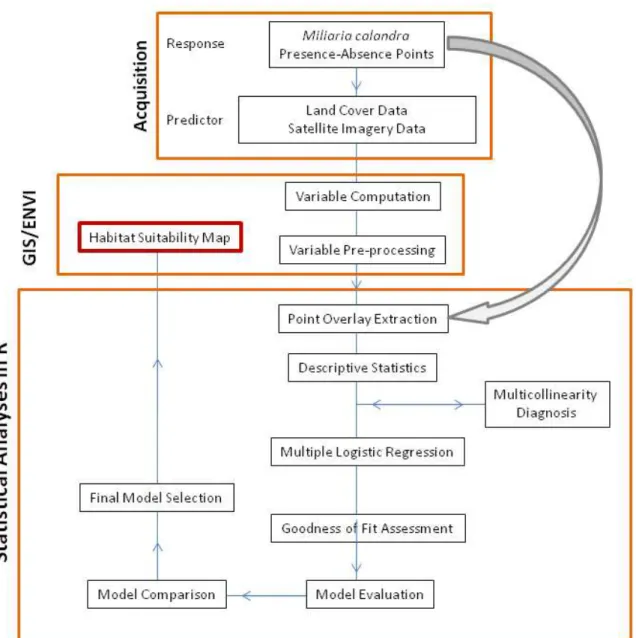
Figure 3: Thesis design flowchart

Figure 4: MSAVI vs. NDVI

Figure 5: NDVI values compared to Land Surface Temperature and Land Surface Emissivity

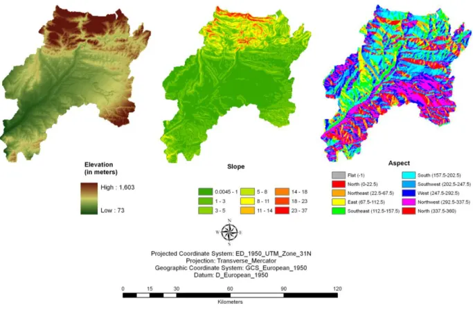
Figure 6: Topographic variables employed in the study

Figure 7: The 27 CORINE Land Cover 2000 classes in the study area.

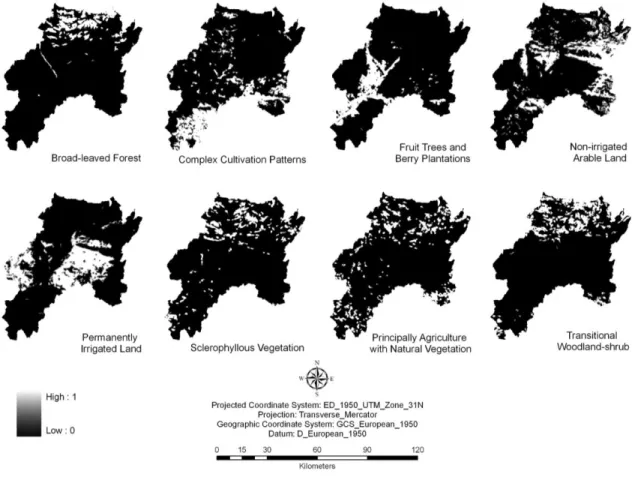
Figure 8: The eight landscape metrics that were extracted from CLC2000

Figure 9: Corn bunting presence-absence points

Figure 10: Habitat suitability map derived from satellite data

Figure 11: Habitat suitability map derived from land cover data

Figure 12: Habitat suitability map derived from a combination of satellite and land cover data

Figure 13: ROC plot of the satellite-only, CLC2000-only and combined model

Figure 14: Comparison between map produced by the Catalan breeding bird atlas and the

final map produced in this study.

Figure 15: Distance to human activity extracted from CLC2000

Figure 16: Distance to roads extracted from CLC2000

Figure 17: Boxplots of the relationship between selected Landsat derivatives and CLC2000

Figure 18: Graphical plots of the association of satellite predictors with the response

Figure 19: Graphical plots of the association of land cover predictors with the response

Figure 20: Graphical plots of the association of anthropogenic predictors with the response

Figure 21: Graphical plots of the association of topographic predictors with the response

(11)

vi

List of Tables

Table 1: Landsat 7 ETM+ band characteristics

Table 2: Tasseled cap transformation coefficients for Landsat ETM+ (Liang 2004)

Table 3: Mean, minimum and maximum values of predictor variables in occupied

squares

Table 4: Results of the bivariate descriptive statistics

Table 5: Summary results of the logistic regression analysis for the satellite model

Table 6: Summary results of the logistic regression analysis for the land cover model

Table 7: Summary results of the logistic regression analysis for the combined model

Table 8: Variance inflation factor values for all the predictor variables

(12)

vii

List of Acronyms

AIC Akaike Information Criterion

AUC Area Under the Curve of the Receive Operating Characteristic AVHRR Advanced Very High Resolution Radiometer

BLF Broad-leaved Forest

CAP Common Agricultural Policy CBBA Catalan Breeding Bird Atlas CCP Complex Cultivation Patterns CLC2000 CORINE Land Cover 2000

CORINE Coordination of Information on the Environment CV Coefficient of Variation

DEM Digital Elevation Model

DN Digital Number

EEA European Environmental Agency EEC European Economic Community EPSG European Petroleum Survey Group ETM Enhanced Thematic Mapper

EU European Union

EVI Enhanced Vegetation Index FTBP Fruit Trees and Berry Plantations GWR Geographically Weighted Regression L1T Level 1 Terrain Corrected

LSE Land Surface Emissivity LST Land Surface Temperature

MSAVI Modified Soil Adjusted Vegetation Index NDVI Normalized Difference Vegetation Index NIAL Non-irrigated Arable Land

NOAA National Oceanic and Atmospheric Administration PANV Principally Agricultural with Natural Vegetation PAR Photosynthetically Active Radiation

PIL Permanently Irrigated Land

R The R Environment for Statistical Computing ROC Receiver Operating Characteristic

SD Standard Deviation

SRTM Shuttle Radar Topography Mission SVEG Sclerophyllous Vegetation

TCT Tasseled Cap Transformation

TM Thematic Mapper

TWS Transitional Woodland-shrub

UK United Kingdom

(13)

viii

Chapter 1 Introduction

1.1 Background and significance

In 1979, the European Economic Community passed the Council Directive

79/409/EEC on the conservation of wild birds, otherwise known as the Birds Directive, which

aims “at providing long-term protection and conservation of all bird species naturally living in the wild within the European territory of the Member States” (EEC 1979). Among other

things, the directive seeks the protection and management of wild birds through the creation

of protected areas and habitat maintenance. However, 25 years after the implementation of

the Birds Directive, farmland bird species and long-distance migrants continue to decrease

at an alarming rate (Birdlife-International 2004). This has been credited to detrimental land

use policies such as the Common Agricultural Policy (Birdlife-International 2004) that have

promoted the intensification of farmlands through crop specialization (monocultures),

pesticide use and the eradication of uncultivated areas in order to maximize productivity

(Donald et al. 2001).

Farming evolved over the last 10,000 years and spread across the forested

European landscape up to the point that over 50% of the European continent is used for

farming. Several organisms have adapted to this new landscape and are now open-country

specialists that use farmland as their primary habitat (Donald et al. 2002). Gradually,

agricultural landscape began to support a large amount of biological diversity and eventually

became its own ecosystem, sustained by humans through traditional farming systems that

employ low-input techniques such as lack of irrigation, large fallow areas and relatively low

potential yields. This habitat supports more bird species of conservation concern than any

other habitat in Europe (Stoate et al. 2003).

1.1.1 The decline of farmland breeding birds in Europe

The decline in farmland bird species first became obvious in the 1980s, which was

the decade that displayed a steady rise in EU agricultural output and the adoption of

(16)

2

of intensive agricultural practices is characterized by a high amount of heavy soils and

extensive irrigation of the landscape which doubles the yield of certain crops (Stoate et al.

2000). In contrast, areas that are extensively farmed are high in biodiversity (Tucker and

Heath 1994; Benton et al. 2003) and are characterized by thin soils, no irrigation, high fallow

areas and low yields (Stoate et al. 2000).

Some species have been extinct as breeders in certain countries; for example the

Red-backed Shrike Lanius collurio in the UK and the Roller Coracias garrulus in the Czech

Republic (Tucker and Heath 1994). While others, such as the Corncrake Crex crex in

France (Deceuninck 1998), have been identified as endangered. The declines in breeding

birds not only have implications for Europe but also contribute to declines in biodiversity for

Africa and Asia as those continents host many migratory European species during winter

months.

Birds are good indicators of the state of the environment because they are highly

mobile, well-studied, easily monitored and occupy a range of habitats (Tankersley 2004;

Gregory et al. 2005). Due to their high mobility, birds can also respond quickly to changes in

landscape and local vegetation (Coreau and Martin 2007; Vallecillo et al. 2008).

Accordingly, it is critical to understand species‟ relationship with their habitats to determine

which areas are more favorable than others. Bird conservation requires spatial information;

this understanding not only serves as a check on the individual species‟ populations but also

as a measure of the overall health of the ecosystem.

The term “bird atlas” has appeared in ornithological vocabulary to mean aggregated distribution maps based on rectangular presence/absence grids produced from field

surveys; currently many countries have their own breeding bird atlases. However, such

projects may take several years to complete and there often is a large temporal lag between

two inventories because it is a time and effort consuming process that is often limited to

small spatial extents (Norris and Pain 2002; St-Louis et al. 2006). Therefore, there is a need

for a rapid and more effective process to map species distributions that is relatively

(17)

3

1.1.2 The Corn Bunting Miliaria (Emberiza) calandra.

The target species in this study is the corn bunting Miliaria calandra (Figure 1), which

is a bird of low-intensity arable landscapes (Taylor and O'Halloran 2002). The northern and

central European corn bunting population has declined sharply since the mid-1970s (Tucker

and Heath 1994) particularly in Britain (Brickle et al. 2000), Poland (Orlowski 2005) and

Ireland (Taylor and O'Halloran 2002) while southern European breeding densities,

particularly in Spain, Portugal and Turkey are stable (Diaz and Telleria 1997). Declines in

northern corn bunting populations have been attributed to the process of farmland

intensification (Brickle et al. 2000; Donald et al. 2001) mentioned in the preceding section.

However, relatively few studies have been conducted on the habitat requirements and

breeding density of corn buntings in southern Europe (Brambilla et al. 2009).

(18)

4

1.2 Species distribution modeling

Birds, like all mobile organisms, have favorite habitats in which to breed, spend

winter months and refuel while on migration. In order to effectively conserve a species it is

vital to know these habitats and their spatial dimensions. Several studies have utilized

geospatial technologies in bird distribution research. However in this thesis only indirect

methods of mapping species will be discussed. Indirect methods involve the use of land

cover mapping and other remote sensing techniques based on habitat requirements to

predict the distribution of species (Nagendra 2001). The advantages of using satellite

imagery include large areal coverage and fine spatial and temporal resolutions (Griffiths et

al. 2000) while national land cover datasets have proven to link birds to habitat classes and

vice versa (Fuller et al. 2005).

St-Louis et al (2006) used linear regression models to evaluate the correlation

between high-resolution satellite image texture and bird point count data, the results have

shown that different methods described 57% to 76% of variability in species richness. A

similar study by Bellis et al (2008) assessed the relationship between greater rhea Rhea

americana group size against normalized difference vegetation index (NDVI) and texture

measures from Landsat Thematic Mapper (TM) imagery. Their results had shown that “rhea

group size was most strongly positively correlated with texture variables derived from near

infrared reflectance measurement”. The use of outputs resulting from the characterization and identification of upland vegetation using satellite imagery in bird abundance–habitat

models was performed by Buchanan et al (2005). Their results showed that bird

abundances forecasted using Landsat Enhanced Thematic Mapper (ETM) derived

vegetation data was similar to that acquired when field-collected data were used for one bird

species.

A study on the use of unclassified satellite imagery in the study of habitat selection of

three bird species was undertaken by Erickson et al (2004) in a method that uses Landsat

TM spectral values. Foody (2005) applied geographically weighted regression (GWR) on

NDVI and temperature variables derived from Advanced Very High Resolution Radiometer

(19)

5

indicated the ability to characterize aspects of biodiversity from coarse spatial resolution

remote sensing data and highlight the need to accommodate for the effects of spatial

non-stationarity in the relationship. Wallin et al (1992) monitored potential breeding habitat for

the red-billed quelea Quelea quelea using NDVI calculations derived from AVHRR.

A combination of land cover maps derived from Landsat ETM imagery, digital

elevation models (DEM) were utilized by Hale (2006) to model the distribution and

abundance of Bicknell‟s thrush Catharus bicknelli that resulted in spatially explicit

predictions of probability of species‟ presence. Habitat selection criteria for the loggerhead shrike Lanius ludovicianus were derived from one province and applied to Landsat TM

imagery covering another province by Jobin et al (2005) in order to evaluate the availability

of suitable breeding habitats. Laurent et al (2005) investigated the potential of using

unclassified spectral data in the predicting the distribution of three bird species using

Landsat ETM imagery and point count data.

The effectiveness of combining Landsat TM satellite imagery, topographic data and a

Geographic Information System (GIS) in bird species richness modeling was investigated by

Luoto et al (2004) where they concluded that a spatial grid system containing different

environmental variables derived from remote sensing data creates consistent datasets that

can be used when predicting species richness. Nohr and Jorgensen (1997) concluded that

“there is a positive correlation between avian parameters and satellite image features with

the highest value obtained when correlating avian data with combined data from Landsat

TM images on landscape diversity and integrated NDVI (INDVI) derived from AVHRR

imagery”.

Knowledge of the range and distribution of species at risk of extinction is crucial. In

Senapathi et al (2007) the loss of habitat that the critically endangered Jerdon‟s courser

Rhinoptilus bitorquatus suffered from 1991 to 2000 was quantified using classified Landsat

TM and ETM imagery. Their results have shown that the species‟ breeding habitat has been

decreasing at an annual rate of 1.2-1.7%.

Apart from unclassified satellite imagery, habitat variables can be extracted from land

(20)

6

compared the capacity of two general land cover maps and “two more accurate structural vegetation maps” in forecasting the distribution of bird species.

A review of studies in bird-habitat relationships using satellite imagery in the last

thirty years was presented in Gottschalk et al (2005), where 120 publications were

examined. A noteworthy conclusion of the review was that the potential of using the

geospatial tools of remote sensing and GIS “might exist in their application in limited access

ecosystems and where coarse and quick but quantitative estimates with statistical

confidence limits on biodiversity are needed to achieve wildlife conservation and

management objectives”.

1.3 Statement of problem

Conservation work is sometimes done by non-profit organizations that cannot afford expensive methodologies with their limited resources. On the other hand, national

agencies and environmental lobby groups might find themselves in situations that require

the rapid production of results to decision makers. Since Coordination of Information on the

Environment (CORINE) land cover and Landsat datasets are free and bird distribution and

habitat suitability models can be derived from them relatively quickly, they present

themselves as important conservation tools.

The problem is that the potential of public domain data is not fully exploited. Public

data is under-used because of its coarse output compared to more detailed, and more

expensive, data.

Although as Gottschalk (2005) demonstrated, there is no lack in research that deals

with the use of geospatial tools in the prediction of species‟ distribution, there is, however, a

lack in comparative research that assesses land cover data and satellite imagery in habitat

modeling. There is additionally a need to evaluate the viability and accuracy of distribution

maps from public sources because of their potential as primary sources of environmental

(21)

7

1.4 Study area

The study area is located in the province of Lerida in the western part of the

Autonomous Community of Cataluña, Spain. The area is covered by low-intensive cereal

crops and small remains of the original dry-shrub vegetation. The study area covers

approximately 1,514 square kilometers and is a stepic landscape comprised of non-irrigated

cropland and dry forests with land use devoted to extensive agriculture and dry pastureland

(Sundseth and Sylwester 2009). The study area also encompasses part of the Lerida plain,

which is an area of steppes and pseudo-steppes on the eastern edge of the river Ebro basin

(Ponjoan et al. 2008).

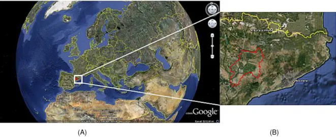
(A) (B)

Figure 2: Overview of the study area in Google Earth. (A): The white box shows location of the study area within Europe. (B): The red outline shows location of the study area within Cataluña.

1.5 Research objectives

Notwithstanding previous research, there is an inadequate amount of information on the

relationship between the occurrence of farmland bird species and predictor variables

extracted from a combination of public domain sources. This study aims to develop a model

of the probability of occurrence of the corn bunting based on habitat preference.

(22)

8

1. Assess the predictive power of variables derived from public domain satellite imagery

and general-purpose land cover data in modeling the distribution of the corn bunting

based on habitat preference.

2. Compare predictions produced by satellite imagery against predictions obtained from

the land cover data.

3. Examine the potential of combining both public data sources in the modeling

process.

1.6 Research questions

1. Can the distribution of the corn bunting be predicted by solely using data derived

from public domain satellite imagery?

2. Can the distribution of the corn bunting be predicted by solely using data derived

from a general-purpose land cover dataset?

3. What is the relative performance of the model resulting from data based on land

cover data against the model resulting from data based on satellite imagery?

4. How does a combined model perform against the individual land cover and satellite

models?

5. Which approach would be more effective in predicting the distribution of the corn

bunting?

1.7 Thesis organization

The design of the thesis encompasses twelve steps that were employed in order to

answer the research questions and fulfill the research objectives. The steps were divided

into three general categories: acquisition, GIS & remote sensing analysis and statistical

analysis. The first category involves the acquisition of the response and the explanatory

predictor variables. The second category involves the computation and extraction of the

predictor raster images using GIS and remote sensing methods. The third category involves

the use of the R in a series of statistical analyses that culminates in the creation of a habitat

(23)

9

(24)

10

Chapter 2 Data

This chapter describes how the predictor variables from satellite imagery and land cover

data were extracted and preprocessed for use in the statistical procedure that follows.

2.1 Satellite imagery

Imagery from the Enhanced Thematic Mapper Plus (ETM+) sensor onboard Landsat

7 satellite was downloaded from the United States Geological Survey (USGS) Global

Visualization Viewer version 7.26. Two scenes from path-198, row-31 for the month of June

(01/06 & 17/06) of the year 2001 were used for this study to temporally coincide with the

survey period. Imagery used is a standard level-one terrain-corrected (L1T) product that has

also undergone radiometric and geometric correction. This product level was chosen

because the L1T correction employs ground control points and digital elevation models to

achieve complete geodetic accuracy (USGS 2009).

Table 1: Landsat 7 ETM+ band characteristics

Band Spatial resolution (m) Lower limit (µm) Upper limit (µm) Bandwidth (nm) Bits per pixel

Gain Offset

1 BLUE 30 0.45 0.52 70 8 0.786 26.19

2 GREEN 30 0.53 0.61 80 8 0.817 26.00

3 RED 30 0.63 0.69 60 8 0.639 24.50

4 NIR 30 0.75 0.90 150 8 0.939 24.50

5 MIR 30 1.55 1.75 200 8 0.128 21.00

6 THERMAL 60 10.40 12.50 2100 8 0.066 0.00

7 MIR 30 2.10 2.35 250 8 0.044 20.34

(25)

11

Atmospheric correction was performed using the Quick Atmospheric Correction

(QUAC) method available in the ENVI 4.7 image processing software. QUAC is a method

for atmospherically correcting multispectral imagery in the visible, near infrared and through

mid-infrared region (0.4 – 2.5 µm). The method was chosen because of its ability to

determine atmospheric compensation parameters directly from information contained within

the scene without the need for ancillary information and also allows for any view or solar

elevation angle resulting in accurate reflectance spectra (ITTVIS 2009). Clouds were

masked and the imagery underwent pixel-by-pixel averaging to produce a single

representative image for the month.

2.2 Satellite imagery preprocessing

2.2.1 Texture analysis

Image texture represents the visual effect produced by the spatial distribution of tonal

variability (pixel values) in a given area (Baraldi and Parmiggiani 1995). Satellite image

texture can thus serve as a substitute for habitat structure because variability in the

reflectance among adjacent pixels can be caused by horizontal variability in plant growth

(St-Louis et al. 2009). Due to the size of the study area, a 3x3 pixel local statistic was

selected to calculate first order texture measures of mean, standard deviation and

coefficient of variation. The mean computes the average texture value, the standard

deviation assesses the variability of texture and the coefficient of variation is standard

deviation of pixel values divided by the mean and gives a measure of the variability in image

texture as a percent of the mean. St-Louis et al (2006) has indicated that first order standard

deviation to be the best predictor amongst the first order texture measures.

2.2.2 Calculation of vegetation indices

Photosynthesis in green vegetation requires the absorption of solar radiation in the

region 400–700 nm (called photosynthetically active radiation or PAR) for use as an energy

source (Alados-Arboledas et al. 2000). Beyond the PAR, in the near-infrared region, the

(26)

12

strong difference in absorption and reflectance, a relatively simple algorithm, the Normalized

Difference Vegetation Index (NDVI) was developed (Tucker 1979):

(Equation 1)

Where NIR refers to the near-infrared band (ETM4) and RED refers to the visible red

band (ETM3). The resultant reflectance values are in the form of ratios of the reflected over

the incoming radiation. NDVI ranges between -1 and +1; negative values indicate lack of

vegetation while positive values indicate the presence of vegetation.

NDVI has been proven to be correlated with ecological and physical conditions such

as land cover, vegetation composition, species richness and productivity of many species

(Wallin et al. 1992; Sanz et al. 2003; Seto et al. 2004; Foody 2005; Pettorelli et al. 2005).

Modified Soil Adjusted Vegetation Index (MSAVI) was also added as a predictor

variable because the algorithm possesses a correction factor that can be adjusted according

to vegetation density (Liang 2004; Qi et al. 1994). MSAVI has been shown to enhance the

dynamic range of the vegetation signal, producing greater vegetation sensitivity (Qi et al.

1994). It is defined as:

(Equation 2)

The correction factor (0.5) is generally used for most applications and represents

areas with intermediate vegetation densities. The amount of detail produced by MSAVI

(27)

13

Figure 4: MSAVI vs. NDVI

2.2.3 Tasseled cap transformation

The tasseled cap transformation (TCT; Crist and Kauth 1986) translates multispectral bands

into a feature space that denotes the physical characteristics of the ground cover (Liang

2004). TCT returns six bands, the first three of which: brightness, greenness and wetness

are of relevance. The brightness band corresponds to overall reflectance, greenness is a

measure of vegetation health and structure and the wetness band measures soil moisture

and vegetation density (Crist 1983). The first three TCT bands have been shown to explain

up to 97% of the spectral variance in individual Landsat scenes (Huang et al. 2002) and

(28)

14

Table 2: Tasseled cap transformation coefficients for Landsat ETM+ (Liang 2004)

Feature Band 1 Band 2 Band 3 Band 4 Band 5 Band 7

Brightness 0.3561 0.3972 0.3904 0.6966 0.2286 0.1596 Greenness -0.3344 -0.3544 -0.4556 0.6966 -0.0242 -0.2630

Wetness 0.2626 0.2141 0.0926 0.0656 -0.7629 -0.5388 Fourth 0.0805 -0.0498 -0.1050 -0.1327 -0.5752 -0.7775 Fifth -0.7252 -0.0202 0.6683 0.0631 -0.1494 -0.0274 Sixth 0.4000 -0.8172 0.3832 0.0602 -0.1095 0.0985

2.2.4 Land surface temperature

The first step of obtaining LST involves accounting for the land surface emissivity

(LSE) of the study area. Surface emissivity is a quantification of the intrinsic ability of a

surface in converting heat energy into above-surface radiation and depends on the physical

properties of the surface and on observation conditions (Sobrino et al. 2001). LSE was

calculated following the procedure by Sobrino et al (2004).

LSE can be extracted by using NDVI considering three different cases (1) bare

ground (2) fully vegetated and (3) mixture of bare soil and vegetation (Sobrino et al. 2004).

Since the study area falls within the third case, the following equation is used to extract LSE:

(Equation 3)

Where

ε

is the LSE and Pv is the proportion of vegetation obtained and is calculated by:

(Equation 4)

Where :

(29)

15

The next step involves calculating the at-sensor radiance (L_λ), which is the amount of energy that reaches the satellite sensor:

(Equation 5) Where:

DN = the quantized calibrated pixel value in DN

LMin = the spectral radiance that is scaled to QCalMin in watt/m2 * ster * µm LMax = the spectral radiance that is scaled to QCalMax in watt/m2 * ster * µm

QCalMin = the minimum quantized calibrated pixel value (corresponding to LMin) in DN QCalMax = the maximum quantized calibrated pixel value (corresponding to LMax) in DN

The at-sensor radiance is in turn converted to the effective at-satellite temperatures

of the viewed Earth-atmosphere system under an assumption of unity emissivity (USGS

2009). This is also referred to as blackbody temperature and denotes a surface that absorbs

all the electromagnetic radiation that reaches it. The blackbody temperature is calculated by:

(Equation 6) Where:

K1 = Calibration constant 1 (666.09 watt/m2 * ster * µm)

K2 = Calibration constant 2 (1282.71 K)

Lλ= At-sensor radiance calculated from Equation 5.

A final step involving correction for spectral emissivity is necessary according to the

(30)

16

(Equation 7) Where:

TB = Blackbody temperature from Equation 6.

λ = Wavelength of emitted radiance (11.5 µm)

ρ = h x c/σ =1.438 x 10-2 mK (σ=Boltzmann constant=1.38 x 10-23 J/K, h=Planck‟s constant=6.626 x 10-34 Js, c=velocity of light=2.998 x 108 m/s)

lnε = Land surface emissivity calculated from Equation 3. TM6 = Landsat thermal band 6 in DN

All LST retrieval algorithms and descriptions apart from LSE estimation are

according to the Landsat Science Data User‟s Handbook (USGS 2009)

(31)

17

2.2.5 Topographic variables

Topography indirectly affects the distribution of species by modifying the relationships of

birds with vegetation or by modifying the vegetation types (Seoane et al. 2004a). Shuttle

Radar Topography Mission (SRTM) digital elevation model (DEM) resampled to 250m was

downloaded from the CGIAR-CSI database.

Figure 6: Topographic variables employed in the study

2.3 Land cover data

CORINE Land Cover (CLC) data for the year 2000 (CLC2000; dated 01/01/2002)

was downloaded from the EEA‟s online portal. CLC is a pan-European project that aims to produce distinctive and comparable land cover data set for Europe. CLC has a total of 44

(32)

18

2.4 Land cover data preprocessing

2.4.1 Anthropogenic variables

Anthropogenic factors such as road density are important measures for predicting bird

assemblages in agricultural eco-regions (Whited et al. 2000). A vector shapefile of the major

roads in the study area was obtained from ESRI Data and Maps 2002 and the Euclidian

distance to roads was calculated. One anthropogenic factor was extracted from the land

cover map: distance to human activity. This was done by rasterizing the CLC2000 map and

extracting only the CLC codes which correspond to human activity:

 Continuous urban fabric

 Discontinuous urban fabric

 Industrial or commercial units

 Construction sites

 Mineral extraction sites

This was followed by calculating the Euclidian distance of each pixel to the above land cover

classes. Due to space limitations, the figures of the anthropogenic variables are exhibited in

(33)

19

Figure 7: The 27 CORINE Land Cover 2000 classes in the study area.

2.4.2 Landscape metrics

Landscape metrics are indices developed for categorical map patterns that quantify

specific spatial characteristics of patches, classes of patches, or entire landscape mosaics

(Smith et al. 2003). They help explain how spatial patterns of landscapes influence the most

important ecological processes (Carrao and Caetano 2002) and have also been applied in

an urban context (Cabral et al. 2005).

Compositional metrics were calculated from the CLC2000 data and included the

proportions of habitat types and landscape richness. Local statistics were calculated using a

3x3 pixel moving window to quantify the landscape metrics with 0 signifying the absence of

the metric in the window and 1 signifies that the window is fully covered by the metric

(34)

20

 Broad-leaved Forest

 Complex Cultivation Patterns

 Fruit Trees and Berry Plantations

 Non-irrigated Arable Land

 Permanently Irrigated Land

 Sclerophyllous Vegetation

 Principally Agricultural with Natural Vegetation

 Transitional Woodland-shrub

(35)

21

2.5 Catalan breeding bird atlas

Data was provided by the Catalan breeding bird atlas (CBBA) in the form of

presence/absence records of eight bird species. Surveys were conducted in the summer

breeding season (March 1st to July 30th) in the years 1999-2002. Surveys were conducted between sunrise and 11 am, and between 6 pm and sunset. The survey plots were 1 km ×1

km UTM squares in which two 1-hour surveys were conducted and the presence or absence

of each species recorded. The CBBA does not allow the use of tapes or lures to increase

the attract species (Brotons et al. 2008). The assignment of the category “Confirmed Breeding” was performed following guidelines set by the European Ornithological Atlas

Committee and includes (Brotons et al. 2008):

 Anti-predatory displays

 Nest used during current breeding season

 Recently fledged young

 Adult carrying fecal sacs or food

 Nest with eggs or bird incubating

 Nest with young; or young of nidifugous species

Since the records of all eight bird species were spread out over the five months and indeed

over all four years, a subset of one farmland species, the corn bunting Miliaria calandra was

(36)

22

Figure 9: Corn bunting presence-absence points

2.6 Analysis tools

The primary tool for statistical analysis is the R Environment for Statistical Computing

version 2.9.2 (R Development Core Team 2009) using the R Commander graphical user

interface version 1.5-3 (Fox 2005). Open Office 3.1 was used to manipulate tabular data.

GIS analysis, creation and visualization of predictive surfaces were conducted using ArcGIS

9.3. Satellite image analysis was done in ENVI 4.7. The EPSG:23031 projection was

retrieved from the EPSG list provided in the rgdal package (Bivand et al. 2008; Keitt et al.

(37)

23

Chapter 3 Methodology

This chapter describes the statistical analyses that were employed to produce

probability maps of the occurrence of the corn bunting based on habitat preference. In this

and subsequent chapters, the statistical terminology „response variable‟ refers to the corn

bunting. It is the target species whose response was modeled based on a set of predictor

variables. The entire R code used in this study is presented in Appendix D.

3.1 Bivariate descriptive statistics

Bivariate descriptive statistics were calculated to gauge the relationship between

each predictor and the response variable. Furthermore, the relationship of satellite

derivatives with the land cover codes is presented in Appendix B.

Regression coefficients explain the amount of contribution of each predictor variable

in terms of the log odds of the response variable. A positive coefficient expresses a directly

proportional relationship while a negative coefficient expresses an inversely proportional

relationship. The magnitude of the coefficient describes the strength of influence of that

predictor variable. The standard error assesses the precision of the regression coefficient

measurements and is an approximation of the standard deviation of the coefficients. The

Z-value is basically the Z-value of each coefficient divided by its standard error. The square of

the Z-value is approximately a chi-square statistic with one degree of freedom called the

Wald statistic (Kleinbaum and Klein 2002). The presence of high multicollinearity between

the predictor variables causes an inflation of the standard errors causing lower values of the

Wald statistic and creating Type II errors (Menard 2002). A p-value of 0.05 means that there

is 5% likelihood that the model results would be produced in a random distribution, so there

(38)

24

3.2 Multiple logistic regression

The statistical method employed in this study is multiple logistic regression. There

are several statistical methods that use binary data for mapping the distribution of species

based on habitat preference. However, they exhibit certain drawbacks.

Artificial neural networks (ANN) demonstrate a good predictive capability but an

assessment of the relative contribution of the predictors is quite difficult. Methods such as

ecological niche factor analysis (ENFA; Hirzel et al. 2002) offered in the Biomapper

software, while offering good predictions, obscures the internal workings of the algorithm so

the process which has resulted in the predictions is unclear. Others such as genetic

algorithm for rule-set prediction (GARP; Stockwell and Peters 1999) use presence-only data

and create random pseudo-absences for presence-absence modeling. The flaw in this

method is that pseudo-absences points might be allocated to areas that possess favorable

habitats. Brotons et al (2004b) have shown that the use of recorded absence data yields

better predictions than pseudo-absences and they recommend their inclusion into habitat

modeling algorithms.

Therefore logistic regression, implemented through R, stands out as a viable method

that offers the combination of methodological transparency, assessment of predictor

contribution, and allows the use of recorded absence data.

Logistic regression is a binomial generalized linear model that predicts the probability

of occurrence of an event using a binary response variable and multiple covariates (Hosmer

and Lemeshow 2000). The probability distribution is fitted to the sigmoid logistic curve and

the outcome is between 0 and 1. Imagine that π is the probability of an event occurring,

hence the logit of Y from a set of predictor variables (X1… Xn) is:

(39)

25

Where b0 is a constant (the y-intercept) and b1, b2, b3… bn are the regression coefficients

estimated by the maximum likelihood method. The formula above states that the response

variable represents the input of all the variables in the model. The response is transformed

to a logit variable and a maximum likelihood approximation is implemented. The logit

variable is the natural log of the odds of the response being 1 or 0, hence estimating the

odds whether an event (represented by the response) will occur. Hence, the probability of Y

occurring is given by:

(Equation 9)

The logistic models were fitted using the glm function of the stats (R Development Core

Team 2009) package.

3.3 Multicollinearity diagnosis

Multicollinearity refers to extreme correlation between the predictor variables. This

leads to a situation where the regression model fits the data well, but none of the predictors

has any significant impact in predicting the dependent variable because they basically share

the same information (Ho 2006). Sometimes predictors in high correlation that individually

explain a significant portion of deviance can appear non-significant due to the collinearity

(Guisan et al. 2002). Pearson correlation coefficients can be computed using the cor

function in R, however that pair-wise approach is limited to only two variables at a time and

does not account for correlation between multiple variables. Therefore, the variance inflation

factor, VIF (Brauner and Shacham 1998) has been computed for each variable to detect

multicollinearity. VIF is calculated as:

(40)

26

The expression 1-R2 is the tolerance and R2 is the proportion of variance the predictor variables explain in the response variable. The function vif in the Design package (Harrell

2009) was used to compute VIF values.

3.4 Variable selection

Models that have too few predictor variables can introduce bias in the inference process,

while models that possess too many variables could yield poor precision or identification of

effects that are actually non-existent (Burnham and Anderson 2004). Since there are several

derivatives of Landsat bands in use, the problem of multicollinearity can lead to a high

degree of unreliability in the estimated regression coefficients (Kleinbaum and Klein 2002),

therefore the satellite model underwent a stepwise selection process to pick variables that

significantly contribute to the model‟s ability to describe the data. All the satellite predictor

variables were placed in the model and then an iterative forward-backward elimination

(Pearce and Ferrier 2000a) of the non-significant variables was performed. Then, variables

with high VIF values were removed one at a time until all the variables have VIF values

below 10 which is the threshold below which multicollinearity is not of concern (Brauner and

Shacham 1998).

3.5 Assessing goodness of fit and model validation

A goodness of fit assessment describes how well a given model fits the data by

measuring the deviation between observed values and the values produced by the model.

Two measures of goodness of fit are used here: Pearson Chi-square and the Likelihood

ratio test.

Pearson Chi-square (χ2) test statistic evaluates H0 that the independent variables are not

in a linear relationship to the log-odds of the response. This test evaluates improvement

(41)

27

(Equation 11)

Where O the observation, E is the expectation, n is the amount of possible results.

Logistic models provide a better fit to the data if improvement over the null model is

exhibited (Hosmer and Lemeshow 2000). The likelihood ratio test is based on the disparity

between deviance of the intercept-only model minus the deviance of the full model. The test

was performed using the lrtest function of the lmtest package (Zeileis and Hothorn

2002). Likelihood is the probability of the response‟s observed values to be predicted from

the predictor variables. The likelihood ratio test statistic is given by:

(Equation 12)

Where L1 and L2 denote the maximized likelihood values for models 1 and 2 respectively;

this is a distributed statistic with degrees of freedom equal to the number of predictors

and is a measure of how poorly the model predicts the decisions. It is a probability that

ranges from 0 to 1.The log likelihood of this probability produces a value between 0 for no

significance, and for high significance, however by multiplying that value by –2, the high

significance value would be .

In ordinary least squares, the coefficient of determination, R2, serves as a statistic that ranges from zero to one and summarizes the overall strength of a given model. There is no

such statistic for logistic regression but a number of pseudo-R2 statistics have been proposed in the last three decades (Hu et al. 2006). One of them, the Nagelkerke R2, implemented through the lrm function in the Design package (Harrell 2009), is used here.

(42)

28

The model performance is estimated by measuring the true error rate. The predicted

probabilities of the chosen models are corroborated with the actual values to determine if

high probabilities are associated with incidents (1) and low probabilities with non-incidents

(0). Since the dataset has quite a limited set of observations, a cross validation resampling

technique was chosen to evaluate performance. The K-Fold Cross-Validation performs K

random splits of the dataset, with each split retained for testing and the remaining K-1 for

training. By training and testing the model on separate subsets of the data, an idea of the

model's prediction strength is obtained (Tibshirani and Tibshirani 2009). Each K-1 split

produces an error rate; hence, the true error (E) is estimated as an average of the separate

error rates:

(Equation 13)

The benefit of this method is that all records are used for both training and testing. The

cross validation was performed using the cv.glm function in the boot package (Canty and

Ripley 2009).

3.6 Model evaluation and selection

Model predictive power was evaluated using area under the curve (AUC) of the receiver

operating characteristic (ROC) which relates sensitivity (true positive) on the y-axis against

the corresponding 1 minus specificity values (false positive) on the x-axis for a wide range of

threshold levels (Pearce and Ferrier 2000b). The closer the AUC value is to 1.0, the better

the model performance. The AUC index is significant due to the single measure of general

accuracy it provides that is not reliant on a particular threshold (Deleo 1993). AUC analysis

was performed using functions in the Presence-Absence package (Freeman and Moisen

(43)

29

Models were compared using the Akaike Information Criterion, AIC (Akaike 1973) which

offers a clear-cut comparison between models that is not reliant on a hypothesis testing

context (Burnham and Anderson 1998). This method is preferred because it extracts more

information from the data regarding the relative strength of evidence for each variable and

model (Young and Hutto 2002). AIC is described by the following formula:

(Equation 14)

The first part, A, is the probability of the data given a model and the second part, b, is the

number of parameters in the model. The first part approximates how well the model fits the

data. The second part is a penalty which relies on the number of parameters used. Smaller

(44)

30

Chapter 4 Results

4.1 Overlay analysis

The corn bunting occupies 251 1x1 UTM squares which represents 73.8% of the total

number of squares in the study area. The predictor variables in the form of ASCII files were

imported into R using the readGDAL function of the rgdal package (Keitt et al. 2009) and

corn bunting presence points were then overlaid on the ASCII files using the overlay

function of the sp package (Pebesma and Bivand 2005). Table 3 shows the mean, minimum

and maximum of the predictor variables in the occupied squares.

Table 3: Mean, Minimum and Maximum values of predictor variables in occupied squares

Variable Mean Min Max Variable Mean Min Max

(45)

31

4.2 Bivariate descriptive statistics

Bivariate descriptive statistics involves concurrently examining two variables to

conclude if there is a relationship between them (Appendix B). The results of the descriptive

statistics are summarized in Table 4. The regression coefficients produced by NDVI and

MSAVI have strong positive correlation with the response variable. The Non-irrigated Arable

Land (NIAL) coefficient also produced strong positive correlation while Broad-leaved forest

(BLF) and Transitional Woodland Shrub (TWS) coefficients produced strong negative

correlation with the response variable which is reasonable considering the fact that corn

buntings strongly favor open arable landscape and avoid wooded areas. All the predictors

that produced strong correlation with the response also exhibited low (<0.05) p-values.

Table 4: Results of the bivariate descriptive statistics

Variable Coefficient S.E. Z p-Value Variable Coefficient S.E. Z p-Value

(46)

32

4.3 Satellite model

The minimal adequate model for the satellite predictor variables is summarized in

Table 5 and the resultant map in Figure 10. The selected model contains seven predictor

variables.

Table 5: Summary results of the logistic regression analysis for the satellite model

Coefficient S.E. Z p-Value

(Intercept) -12.74107 3.00470 -4.24000 0.0002 band4m 0.04256 0.01538 2.76700 0.00565 msavi_m 3.43200 0.97912 3.50500 0.00046 band1sd -0.09312 0.05626 -1.65500 0.09787 band5cv 5.25594 1.73581 3.02800 0.00246 dem 0.00319 0.00126 2.52900 0.01144 slope -0.30126 0.07579 -3.97500 0.00007 lst 0.28615 0.07197 3.97600 0.00007

ND 388.24 df 338

RD 302.81 df 331

AIC 318.81

Pearson ChiSq 92.4039 PCC 0.7905

L.R. 85.43 AUC 0.8095

R2 0.331 CV Error 0.1520

The AUC value for this model was 0.81 with 79% of the points accurately classified.

The Nagelkerke pseudo-R2 statistic was 0.33 (95% Confidence Interval: 0.251

≤

R2

≤

0.410), which means that approximately 33% of the variation in the response is explained by

the model. K-Fold Cross Validation yielded an error rate of 0.15. The model performed 30%

better than a random model. The residual deviance (318.81) is well below the degrees of

freedom (331) indicating that there is no over-dispersion in the model.

The importance of each variable is presented in visual form in Appendix C using

(47)

33

(48)

34

4.4 Land cover model

The logistic regression model for the land cover predictor variables is summarized in Table 6

and the resultant map in Figure 11. The selected model contains eight predictor variables.

Table 6: Summary results of the logistic regression analysis for the land cover model

(Intercept) -0.70370 0.45650 -1.542 0.12320 panv 1.20700 0.86130 1.401 0.16120 ccp 1.13600 0.53980 2.105 0.03530 ftbp 1.29100 0.61390 2.103 0.03550 nial 4.03200 0.72160 5.587 2.31E-008

pil 2.39500 0.55740 4.297 0.0002 sveg 1.92400 0.97690 1.970 0.04890 humdist -0.00008 0.00005 -1.687 0.09170 wetdist 0.00005 0.00002 2.394 0.01660

ND 388.24 df 338

RD 304.17 df 330

AIC 322.17

Pearson ChiSq 88.0229 PCC 0.7964

L.R. 84.07 AUC 0.8103

R2 0.322 CV Error 0.1543

The AUC value for this model was 0.81 with 79.6% of the points accurately

classified. The Nagelkerke pseudo-R2 statistic was 0.32 (95% Confidence Interval: 0.242

≤

R2

≤

0.401), which means that approximately 32% of the variation in the response is explained by the model. K-Fold Cross Validation yielded an error rate of 0.15. The model

performed 31% better than a random model. The residual deviance indicates the absence of

over-dispersion.

Because of the coarse resolution of the CLC2000, the probability map comes out

coarse as well. Although the land cover map does provide valuable information it is not as

(49)

35

even without the topographic data the land cover model assumes an unfavorable habitat in

the higher altitudes with steep slopes.

The importance of each variable is presented in a visual form in Appendix C using

plot.anova.Design function.

(50)

36

4.5 Combined model

The logistic regression model for the combined predictor variables is summarized in Table 7

and the resultant map in Figure 12. The selected model contains twelve predictor variables.

Table 7: Summary results of the logistic regression analysis for the combined model

(Intercept) -12.16 3.49500 -3.48 0.0050 band4m 0.02018 0.01692 1.193 0.23285 msavi_m 3.28700 1.08300 3.034 0.00241 band1sd -0.14150 0.06071 -2.331 0.01974 band5cv 4.60000 1.85600 2.478 0.01320 dem 0.00262 0.00145 1.802 0.07152 slope -0.21100 0.08201 -2.573 0.01008 lst 0.32840 0.09584 3.426 0.00061 nial 1.97500 0.61340 3.220 0.00128 pil 1.65800 0.68590 2.417 0.01566 sveg 1.63300 1.06100 1.539 0.12387 humdist -0.00009 0.00005 -1.762 0.07812 wetdist 0.00004 0.00002 1.677 0.09360

ND 388.24 df 338

RD 276.11 df 326

AIC 302.11

Pearson

ChiSq 90.6919 PCC 0.8171

L.R. 112.13 AUC 0.8462

R2 0.413 CV Error 0.1433

The AUC value for this model was 0.84 with 81.7% of the points accurately

classified. The Nagelkerke pseudo-R2 statistic was 0.41 (95% Confidence Interval: 0.335

≤

R2

≤

0.490), which means that approximately 41% of the variation in the response is explained by the model. K-Fold Cross Validation yielded an error rate of 0.14. The model

performed 35% better than a random model. The saturated model with all 39 variables

(51)

37

(RD=240.19) due to the number of parameters in the model because deviance corresponds

to −2 times the log likelihood of the data under the model and measures how the model predicts the decisions. Since smaller residual deviance is better, it is tempting to select this

model, however, the p-values and the inflated standard errors due to the presence of

multicollinearity has led to its rejection.

(52)

38

4.6 Model selection

A comparative receiver operating characteristic (ROC) plot provided in Figure 13 displays

the performance of the combined model in relation to the satellite and land cover models.

Figure 13: ROC plot of the satellite-only, CLC2000-only and combined model

The value of the area under the ROC (AUC) measures the ability of the model‟s predictions

to distinguish between positive and negative cases and hence evaluates the predictive

accuracy of the model. The ROC curve that is closest to the upper-left corner of Figure 13 is

the one with the best predictive performance. The combined model (AUC=0.85) has a better

predictive performance than the other two. Additionally, this model explains more variation

(R2=0.41) in the response than the other two models and has a lower cross validation error rate (E=0.1433). The AIC of the combined model is (AIC=302.11) which is much lower than

the satellite (AIC=318.81) and the land cover (AIC=322.17) models. Based on these facts

(53)

39

Chapter 5 Discussion

This chapter will discuss in detail the results obtained. The satellite model will be discussed

in the first section, followed by the land cover model and the final combined model. The

fourth section talks about the importance of selecting viable predictor variables. The last

section compares the final model from this study and the final corn bunting probability map

from the Catalan breeding bird atlas.

5.1 Satellite imagery

Amongst the satellite variables, land surface temperature (LST: p=0.00007) had the

strongest influence on the corn bunting because of the variable‟s ability in discriminating the

thermal signature of dry, non-irrigated arable land. Additionally, intensified agricultural fields

exhibit low temperature in summer breeding months due to heavy irrigation; therefore, LST

has potential, in dry environments such as Lerida, to discriminate favorable habitats from

non-favorable ones for species such as the corn bunting.

The mean value of the near infrared band 4 (band4m: p=0.0056) and the coefficient of

variation (CV) of the mid-infrared band 5 (band5cv: p=0.0024) exhibited a strong positive

correlation and high significance in describing the corn bunting occurrence. Band 4 is

responsive to photosynthetically active vegetation and the quantity of biomass while band 5

is responsive to vegetation moisture content (St-Louis et al. 2009). This suggests that

texture features in the infrared region are likely to detect variation in vegetation structure.

An interesting result was the relationship of the corn bunting with the standard deviation

of band 1 (band1sd: p=0.097), removal of this variable increased both the residual deviance

and AIC score. The bunting had a negative relationship with band1sd because the spectral

range of band 1 (0.45-0.52µm) is ideal for detecting urban and man-made features.

However a surprising outcome was the exclusion of NDVI from the final model due to its

insignificance (p=0.799), one possible reason can be attributed to the overlap in information

(54)

40

Several satellite variables were excluded from the final models because of the high level

of multicollinearity between them. One approach that might address this inconvenience

would be to use groups of satellite derivatives in separate models as it would reduce the

correlation between different textures of the same band and ensure distinct contribution of

each variable.

5.2 Land cover dataset

The CLC2000 dataset, despite (or because of) being public domain, has a couple of

disadvantages. For starters it takes several years to produce one country-wide (and indeed

Europe-wide) CLC2000 dataset as only three (1990, 2000, and 2006) have been produced

in the last 20 years. And secondly, because of the low resolution, CORINE does not

discriminate between the differences in vegetation structure. These are the areas where

satellite imagery outperforms land cover data due to the high temporal and spatial resolution

of available satellites.

Although the creation of reliable land cover datasets is both time and effort (e.g.

ground-truthing) consuming, the lure of new, more efficient classification algorithms, expert

knowledge, in-field verification make them a promising products in identifying species‟

habitat requirements. In order to be effective, they need to be produced on a yearly basis so

that temporal variations in species‟ habitat preference could be recorded.

5.2.1 Non-irrigated arable land

There was a distinctive preference for non-irrigated arable land (NIAL: p=2.31E-008)

landscape metric which is corroborated by earlier research (Diaz and Telleria 1997; Stoate

et al. 2000; Brambilla et al. 2009). The exclusion of NIAL had the greatest effect on the

model, increasing the AIC by an average of 43.56 and the deviance by an average of 41.56

in the stepwise variable selection process.

5.2.2 Permanently irrigated land

Permanently irrigated land metric (PIL: p=0.0002) is an interesting category because it is

Investigating Habitat Association of Breeding Birds Using Public Domain Satellite Imagery and Land Cover Data

Investigating Habitat Association

of Breeding Birds Using Public

Domain Satellite Imagery and

Land Cover Data

Abdulhakim Mohamed Abdi

Investigating Habitat Association of Breeding

Birds Using Public Domain Satellite Imagery and

Land Cover Data

A Case of the Corn Bunting

Miliaria calandra

in Spain

Programme Title

Geospatial Technologies

Degree

Master of Science

Course Duration

September 2008

–

March 2010

Erasmus Mundus Consortium Partners

Institut für Geoinformatik

Universität Münster, DE

Instituto Superior de Estatística e Gestão de Informação

Universidade Nova de Lisboa, PT

AUTHOR'S DECLARATION

Abstract

Acknowledgements

Dedication

List of Figures

List of Tables

List of Acronyms

Table of Contents

Chapter 1 Introduction

1.1 Background and significance

1.2 Species distribution modeling

1.3 Statement of problem

1.4 Study area

1.5 Research objectives

1.6 Research questions

1.7 Thesis organization

Chapter 2 Data

2.1 Satellite imagery

2.2 Satellite imagery preprocessing

ε

2.3 Land cover data

2.4 Land cover data preprocessing

2.5 Catalan breeding bird atlas

2.6 Analysis tools

Chapter 3 Methodology

3.1 Bivariate descriptive statistics

3.2 Multiple logistic regression

3.3 Multicollinearity diagnosis

3.4 Variable selection

3.5 Assessing goodness of fit and model validation

3.6 Model evaluation and selection

Chapter 4 Results

4.1 Overlay analysis

4.2 Bivariate descriptive statistics

4.3 Satellite model

≤

≤

4.4 Land cover model

≤

≤

4.5 Combined model

≤

≤

4.6 Model selection

Chapter 5 Discussion

5.1 Satellite imagery

5.2 Land cover dataset