HESSD
6, 791–841, 2009
Snow cover data (MODIS) for water balance applications
A. Gafurov and A. B ´ardossy
Title Page
Abstract Introduction
Conclusions References
Tables Figures
◭ ◮
◭ ◮
Back Close
Full Screen / Esc
Printer-friendly Version
Interactive Discussion Hydrol. Earth Syst. Sci. Discuss., 6, 791–841, 2009
www.hydrol-earth-syst-sci-discuss.net/6/791/2009/ © Author(s) 2009. This work is distributed under the Creative Commons Attribution 3.0 License.
Hydrology and Earth System Sciences Discussions
Papers published inHydrology and Earth System Sciences Discussionsare under open-access review for the journalHydrology and Earth System Sciences
Snow cover data derived from MODIS for
water balance applications
A. Gafurov and A. B ´ardossy
Department of Hydrology and Geohydrology, Institute of Hydraulic Engineering, University of Stuttgart, Pfaffenwaldring 61, 70569 Stuttgart, Germany
Received: 6 October 2008 – Accepted: 16 October 2008 – Published: 11 February 2009
Correspondence to: A. Gafurov ([email protected])
HESSD
6, 791–841, 2009
Snow cover data (MODIS) for water balance applications
A. Gafurov and A. B ´ardossy
Title Page Abstract Introduction Conclusions References Tables Figures ◭ ◮ ◭ ◮ Back Close
Full Screen / Esc
Printer-friendly Version
Interactive Discussion
Abstract
Snow cover information is of central importance for the estimation of water storage in cold mountainous regions. It is difficult to assess distributed snow cover information in a catchment in order to estimate possible water resources. It is especially a challenge to obtain snow cover information for high mountainous areas. Usually, snow depth 5
is measured at meteorological stations, and it is relatively difficult to extrapolate this spatially or temporally since it highly depends on available energy and topography. The snow coverage of a catchment gives detailed information about the catchment’s potential source for water. Many regions lack meteorological stations that measure snow, and usually no stations are available at high elevations.
10
Satellite information is a very valuable source for obtaining several environmental parameters. One of the advantages is that the data is mostly provided in a spatially dis-tributed format. This study uses satellite data to estimate snow coverage on high moun-tainous areas. Moderate-resolution Imaging Spectroradiometer (MODIS) snow cover data is used in the Kokcha Catchment located in the north-eastern part of Afghanistan. 15
The main disadvantage of MODIS data that restricts its direct use in environmental applications is cloud coverage. This is why this study is focused on eliminating cloud covered cells and estimating cell information under cloud covered cells using six logical, spatial and temporal approaches. The results give total cloud removal and mapping of snow cover for the study areas.
20
1 Introduction
One of the main sources for water balances of a catchment in a cold environment is snow information. Snow data is especially important in high mountainous areas where snowpack stays for longer periods of time and its melt dominates river discharges in the summer periods. Many data-scarce regions worldwide such as Central Asia greatly 25
HESSD
6, 791–841, 2009
Snow cover data (MODIS) for water balance applications
A. Gafurov and A. B ´ardossy
Title Page Abstract Introduction Conclusions References Tables Figures ◭ ◮ ◭ ◮ Back Close
Full Screen / Esc
Printer-friendly Version
Interactive Discussion in the summer period, which is used to irrigate agricultural fields and for drinking
pur-poses. The importance of snow cover information for environmental studies has been studied by many researchers in the past.
Mapping snow cover with in-situ measurement has already been shown to be im-possible for meso-scale catchments. Remote sensing offers a powerful alternative 5
for obtaining environmental data worldwide. Nowadays, many different instruments are available on satellites that provide continuous information about the earth’s actual state. Moderate-resolution Imaging Spectroradiometer (MODIS) is one such instru-ment installed onboard TERRA and AQUA satellites. Observations were started in February 2000 and July 2002, respectively. These two satellites pass over the equa-10
tor in the morning and afternoon, capturing the earth’s current state twice per day. MODIS uses 36 spectral bands to estimate 44 global data with spatial resolution of up to 250 m. Among other datasets, MODIS also provides gridded snow cover infor-mation in 500 m spatial resolution. The disadvantage of this snow cover data is the failure of clear observation under cloud covered regions. MODIS cannot observe earth 15
coverage through clouds. Nevertheless, MODIS snow cover data has been tested by different researchers with positive results. Among them, Parajka et al. (2006) com-pared MODIS snow cover data with in-situ information over the whole of Austria and reported about 95% agreement between MODIS snow cover and in-situ data from 754 climate stations on cloud free pixels. Klein et al. (2003) reported an 88% agreement 20
when compared with measurements of the Upper Rio Grande Basin. Another study by Tekeli et al. (2005) states that “among 96 observations, 74 observations mapped as snow or land by MODIS agreed with the ground measurements with a matched ratio of 77.08%”.
The limitation of MODIS Snow cover data to be used in hydrological models is the 25
HESSD
6, 791–841, 2009
Snow cover data (MODIS) for water balance applications
A. Gafurov and A. B ´ardossy
Title Page Abstract Introduction Conclusions References Tables Figures ◭ ◮ ◭ ◮ Back Close
Full Screen / Esc
Printer-friendly Version
Interactive Discussion methods to reduce the cloud covered cells from MODIS images. The first is a
combi-nation of Terra and Aqua images, the second is cloud pixel classification according to the majority of eight pixel neighborhoods, and the third is a cloud pixel classification according to the most recent observation of the same pixel. They came up with 9–21% and 6–13% for the first two methods, respectively and different accuracies for the third 5
method according to the temporal approach.
In this study, six methods will be applied to reduce cloud covered pixels from MODIS snow cover data including the combination of Terra and Aqua products as introduced by Parajka et al. The goal is to remove cloud covered cells from snow cover data completely and to map snow coverage over the study catchments.
10
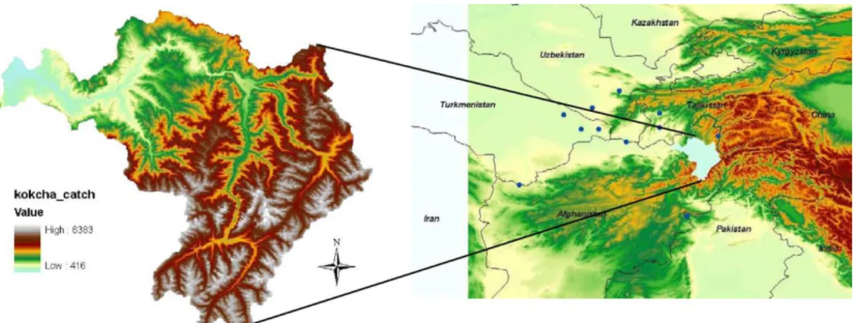
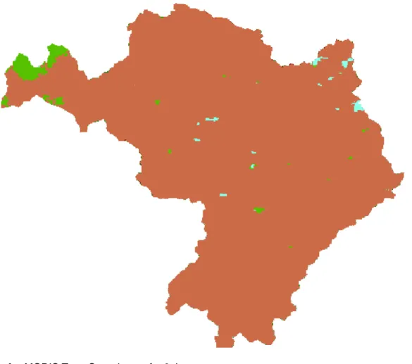
2 Study area
For this research, the Kokcha Basin in the north-eastern part of Afghanistan was cho-sen. It is located from latitude 35.40◦N to 37.40◦N and from longitude 69.30◦E to 71.60◦E, and has an area of 20 600 km2(Fig. 1).
The Kokcha Basin is topographically heterogeneous and its elevation ranges from 15
416 m above sea level (m.a.s.l) in the north-western part to up to 6383 m.a.s.l in the southern mountains. Topographically, about 75% of the basin area is found above 2000 m.a.s.l, about 50% above 3000 m.a.s.l and 30% above 4000 m.a.s.l. The main land cover is grasslands (43%), barren or sparsely vegetated (37%), and open shrub lands (15%). The climate is characterized by semi-arid to arid with hot summers and 20
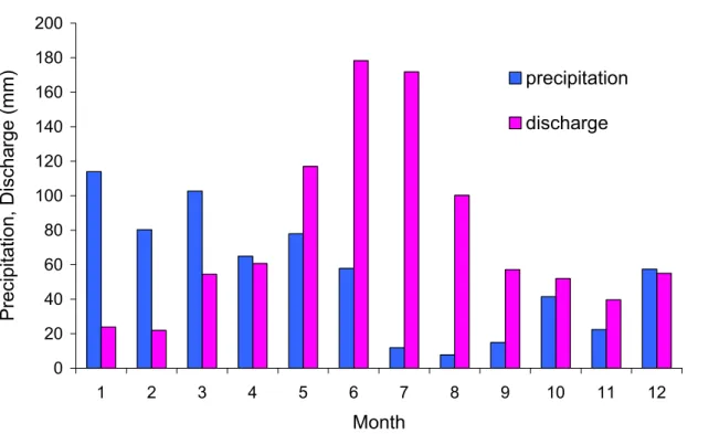
cold winters. It is important to mention that there is almost no precipitation in the summer periods whereas rivers reach their peak record in summer (Fig. 2).
The Kokcha River is the tributary to Pandj River and Pandj River is one of the main water sources for Amudarya, the largest river in Central Asia. Historical discharge anal-yses indicate that about 65% of the total annual volume of water from the Kokcha Basin 25
HESSD
6, 791–841, 2009
Snow cover data (MODIS) for water balance applications
A. Gafurov and A. B ´ardossy
Title Page Abstract Introduction Conclusions References Tables Figures ◭ ◮ ◭ ◮ Back Close
Full Screen / Esc
Printer-friendly Version
Interactive Discussion source for agriculture downstream in the hot summer (over 40◦C) periods. Thus, the
snow data of the catchment is very important when studying the water balances of such region.
3 Data
Moderate-resolution Imaging Spectroradiometer (MODIS) snow cover data is used in 5
this study. This data can be ordered for a certain period or downloaded from a public domain through the Distributed Active Archive Center (DAAC) located at the National Snow and Ice Data Center (NSIDC). MODIS instruments installed in the Terra and Aqua satellites collect data as part of NASA’s Earth Observing System (EOS) program. The first MODIS instrument on the Terra satellite was launched in December 1999 and 10
began to deliver data starting February 2000. The second MODIS instrument on the Aqua satellite was launched in May 2002 and started to deliver data in July 2002. The Terra satellite crosses the equator from south to north at about 10:30 a.m. and the Aqua satellite from north to south at about 1:30 p.m. The Normalized Difference Snow Index (NDSI) is used as the MODIS snow mapping algorithm with a set of thresholds (Hall et 15
al., 2002). More information about the MODIS snow cover algorithm can be found in “MODIS snow cover products” by Hall et al. (2002).
MOD10A1 (MODIS/TERRA SNOW COVER DAILY L3 GLOBAL 500 m SIN GRID V005) snow product with 500 m spatial and daily temporal resolution was obtained for this research in sinusoidal projection. MODIS products are distributed as tiles that have 20
nominal swath coverage of 2330 km (across track) by 2030 km (along track). There is in total 36 horizontal (H) and 18 vertical (V) tiles and the Kokcha Catchment is captured by the H23V05 tile. MODIS data are offered in Hierarchical Data Format (HDF) which can be read by several programs. The MODIS Reprojection Tool (MRT) is used in this study to convert from the HDF format into ArcGIS compatible GEOTIF format. Daily 25
HESSD
6, 791–841, 2009
Snow cover data (MODIS) for water balance applications
A. Gafurov and A. B ´ardossy
Title Page Abstract Introduction Conclusions References Tables Figures ◭ ◮ ◭ ◮ Back Close
Full Screen / Esc
Printer-friendly Version
Interactive Discussion
4 Methodology
In this study, six subsequent approaches are applied in order to eliminate cloud covered pixels and to estimate the pixel cover beyond the cloud covered pixels.
The first approach is the combination of Terra and Aqua satellite images. Since the overpass between the two satellites differs by several hours, it is still acceptable to 5
assume that the snow covered cells from both images should remain the same over the time difference. If the cloud covered pixel of Terra is defined as cloud free in the Aqua pass, then the value of cloud free pixel from Aqua product is accepted as the actual pixel cover. The formula is given in Eq. (1).
S(y,x,t) =maxS(Ay,x,t), S(Ty,x,t) (1)
10
wherey, x, t are vertical, horizontal and temporal indexes of pixelS, respectively. SA
and ST stands for Aqua and Terra pixels, respectively. Equation (1) was applied for both, snow covered and land covered pixels. Maximum snow coverage and maximum land coverage was obtained from two satellite products.
The second approach is the temporal combination of cloud covered pixels. The fact 15
that cloud coverage is always in dynamical movement supports this approach. It can occur that one day is completely cloud covered while the previous or next days are cloud free. This is why in this approach the previous and next days are checked with a one and two days shift. The formula is given in Eq. (2).
S(y,x,t) =1 if (S(y,x,t−1)=1 and S(y,x,t+1)=1) (2)
20
Since the MODIS provides binary information (snow or no snow), 1 corresponds to snow cover and 0 for land cover further in this study. If the Eq. (2) is not fulfilled, then the time step is shifted to one day backwards and forwards as stated in Eqs. (3) and (4).
S(y,x,t)=1 if (S(y,x,t−2)=1 and S(y,x,t+1)=1) (3)
S(y,x,t)=1 if (S(y,x,t−1)=1 and S(y,x,t+2)=1) (4)
HESSD
6, 791–841, 2009
Snow cover data (MODIS) for water balance applications
A. Gafurov and A. B ´ardossy
Title Page Abstract Introduction Conclusions References Tables Figures ◭ ◮ ◭ ◮ Back Close
Full Screen / Esc
Printer-friendly Version
Interactive Discussion Here, the assumption is taken that the snow cover stays more or less constant if the
weather is cloud covered. Solar radiation is the main source for snow melt and if the area covered by snow is cloud covered on that day, which means no solar radiation (at least at the time of the image capturing), then the possible snow melt is neglected. Additional temperature information for those pixels on that day would give more infor-5
mation as to whether there is a possibility for snow to melt or not, but this was not considered in this study.
The third approach is based on snow transition elevation. This approach is well suited for very low and very high located pixels. The concept is to find the minimum and maximum snow covered pixel elevation over a whole catchment for a particular 10
day. These elevation bands are then set as the threshold elevations. All of the cloudy pixels below the minimum snow elevation band should be assigned as land pixels and all pixels above maximum snow elevation band should be assigned as snow covered pixels. The formula is given in Eqs. (5) and (6).
S(y,x,t)=0 if H(y,x)< HminS (t) (5)
15
S(y,x,t)=1 if H(y,x)> HmaxS (t) (6)
where;H(y,x)is the elevation of a pixel at (y, x) location,HminS (t) is the minimum snow covered elevation assuming that there are no snow covered areas below this elevation on dayt and HmaxS (t) is the maximum snow covered elevation on day t. If the whole area contains only snow covered pixels, then this rule does not apply. This approach 20
mainly removes cloudy pixels at very low and very high elevations. It can happen that the top of the mountains are covered by clouds on that day while lower located pixels are defined as snow coverage. In this case, top located pixels should also be covered by snow since the pixels located lower than this cloud covered pixel are covered by snow. It is the same case for land coverage. Very low locations could be defined as 25
HESSD
6, 791–841, 2009
Snow cover data (MODIS) for water balance applications
A. Gafurov and A. B ´ardossy
Title Page Abstract Introduction Conclusions References Tables Figures ◭ ◮ ◭ ◮ Back Close
Full Screen / Esc
Printer-friendly Version
Interactive Discussion The fourth approach is the spatial combination of neighboring pixels. Three direct
neighboring pixels of the cloudy pixel are examined in this approach. If all three pixels are defined as land or defined as snow, then the cloudy pixel is also assumed to be a land or snow pixel.
It is also important to note that this approach may also introduce some minor errors 5
due to the fact that the cloudy pixel may also be land even if three neighboring pixels are snow covered. However, the probability of a pixel being the same as at least three of its direct neighboring cells is higher than it having the opposite coverage than its neighboring cells.
The fifth approach is the combination of neighboring pixels and the elevation between 10
them. In this approach, all neighboring pixels of cloud covered pixel are checked for their coverage. If any of these direct lying neighboring pixels are covered by snow and its elevation is lower than the cloudy pixel, then the cloudy pixel is assigned as having snow coverage as well. This approach is based on the fact that the temperature decreases as elevation increase, and that the snow at higher located pixels should melt 15
after the lower located pixels due to lower energy for melting process. The formula is given in Eq. (7).
S(y,x,t) =1 if (S(y,x+1,t)=1 and H(y,x+1)< H(y,x)) (7)
The sixth approach is based on the time series of each pixel over an entire year. This method checks the day when each pixel is no longer covered by snow. This day is set 20
as “complete snow melt” day and all pixels with the same location before this day are assigned as snow coverage and all pixels after this day are assigned as land coverage. The same rule was applied for snow accumulation period where “snow accumulation start” day was obtained for each pixel using surface cover time series. Figure 3a and b shows an illustration of this method.
25
HESSD
6, 791–841, 2009
Snow cover data (MODIS) for water balance applications
A. Gafurov and A. B ´ardossy
Title Page Abstract Introduction Conclusions References Tables Figures ◭ ◮ ◭ ◮ Back Close
Full Screen / Esc
Printer-friendly Version
Interactive Discussion fall on this pixel starts on the Julian day of 311 (7 November). As shown in Fig. 3b,
the snow completely melts on Julian day of 137 (17 May) and the snow fall starts on the Julian day of 286 (13 October). This analysis was carried out for each pixel and all threshold (snow melt and snow accumulation) days were assigned according to pixel cover information. As a next step, all days for the same pixel before snow melt day and 5
after snow accumulation day were set as snow covered and all days for the same pixel after snow melt day and before snow accumulation day were set as land covered. For the pixel plotted in Fig. 3a, all cloud covered days (value 50) before 1 May and after 7 November were set to be covered as snow and all cloud covered days after 1 May and before 7 November were set as land. The formulas for this approach are given in 10
Eqs. (8) and (9).
S(y,x,t)=1 ∀ tA≤t < tM (8)
S(y,x,t)=0 ∀ tA> t≥tM (9)
where, tM and tA are the threshold days of snow melt and snow accumulation start, respectively and t is day. In order to prevent the error due to present cloud covered 15
cells and also due to the short term snow falls or snow melt, five continuous snow records after the first snowfall were used to decide the snow accumulation day. The same was done for the snow melt period. This step prevents short term snow falls that can be recorded by MODIS and which may melt immediately. Such a day is not assigned as a snow accumulation day since the snow on this day can melt on the next 20
day (no snow cover in time series) and last for several days without snow cover. The same is valid for a snow melt period where five continuous land cover records are used for the threshold (snow melt) day decision. Time series analyses were done from the beginning of the spring season (1 March) to the beginning of the spring season of the next year because of possible large snow fall events happening in winter months. The 25
HESSD
6, 791–841, 2009
Snow cover data (MODIS) for water balance applications
A. Gafurov and A. B ´ardossy
Title Page Abstract Introduction Conclusions References Tables Figures ◭ ◮ ◭ ◮ Back Close
Full Screen / Esc
Printer-friendly Version
Interactive Discussion
5 Results
To illustrate the results, the snow cover product from 8 January 2003 was chosen because this day was one of the cloudiest days recorded by Terra and Aqua satellites. The original MODIS Terra and Aqua snow cover images of the Kokcha Basin for this day are shown in Fig. 4a and b.
5
In the legend, the values 25, 37, 50, 100 and 200 correspond to land, lake or inland water, cloud, snow covered lake ice and snow, respectively. The Terra instrument observed 97.8% cloud cover on this day (8 January 2003) where Aqua with a shift of several hours observes 83.5% cloud cover.
Using the first approach to eliminate cloud covered cells where Terra and Aqua im-10
ages were combined to find best coverage, the cloudy cells were reduced from 97.8% (Terra) and 83.5% (Aqua) to 81.4% as combined. The resulting combination image is plotted in Fig. 5.
Using the second approach where temporal combination of pixels was carried out, the cloud coverage was reduced from 81.4% to 32.6%. This can be counted as one of 15
the days when previous and next days are coarsely cloud covered. The image created after applying this approach is plotted in Fig. 6b.
As it is visible from the image, the 8 January 2003 was one of the most densely cloud covered days as compared to previous and next days (Figs. 5 and 6a and b). This approach is very helpful for such cases where previous and following days are 20
taken into consideration.. The cloud coverage for the days 7 January, 8 January and 9 January before the second stage was 35.2%, 81.4% and 35.1%, respectively. This is why the cloud coverage is reduced from 81.4% to 32.6% in the second approach.
Using the third approach, which is based on snow transition elevation, the cloud coverage was reduced from 33% to 23%. In this case, very high and very low elevation 25
range pixels are corrected to have either snow cover or land cover. The result is plotted in Fig. 7.
HESSD
6, 791–841, 2009
Snow cover data (MODIS) for water balance applications
A. Gafurov and A. B ´ardossy
Title Page Abstract Introduction Conclusions References Tables Figures ◭ ◮ ◭ ◮ Back Close
Full Screen / Esc
Printer-friendly Version
Interactive Discussion The area that is marked by a circle was captured as cloud coverage from the MODIS
instrument and logically should be land coverage because there is no snow presence close to this elevation range. On this day, the minimum elevation where snow was recorded was 2377 m.a.s.l and the percent of area of the Kokcha Basin below this level amounts to 33%. This means that 33% of the Kokcha Basin could logically be 5
estimated to be no cloud covered if there is cloud coverage.
The fourth approach results for the day 8 January 2003 show little improvement. After the implementation of this approach, the cloud coverage was 21% which is slightly different than the previous approach (23%). This approach was based on the spatial combination of neighboring pixels. The result is plotted in Fig. 8.
10
The improvement is not very visible when comparing two images (the one from pre-vious approach and from approach four) for this day. This approach generally resulted in little improvement. In many cases, the average performance over whole year was about 1%.
The fifth approach was based on neighboring pixels and on the pixel elevation. This 15
approach gives a good performance. The cloud coverage was reduced from 21% to 15% for this day. The result is given in Fig. 9.
In this approach, the available energy was considered to assume the pixel cover (snow or land) under cloud coverage. If the neighboring pixel of the cloud covered pixel is covered by snow and its elevation is less than the cloud covered pixel, the cloud 20
covered pixel should also logically be covered by snow due to the fact that less energy is needed for snow melt in upper elevations than in lower elevations.
The last approach considered temporal time series for each pixel. This approach removes all of the cloud from the image. In this approach, threshold melt and snow accumulation dates are calculated for each pixel. The rest of the cloud cover is removed 25
HESSD
6, 791–841, 2009
Snow cover data (MODIS) for water balance applications
A. Gafurov and A. B ´ardossy
Title Page Abstract Introduction Conclusions References Tables Figures ◭ ◮ ◭ ◮ Back Close
Full Screen / Esc
Printer-friendly Version
Interactive Discussion In contrast to the other approaches, this approach is not suitable for operational
pur-poses since it requires melt day and snow accumulation day which may lie at present. It could be yet for operational purposes if the melt day or snow accumulation day is behind. This could work at the end of the year where snow melt day (occurring mostly in spring months) can be obtained and clouds could be eliminated from snow product 5
for spring and summer periods. Using these six approaches, all cloud covered pixels are replaced with non-cloudy pixels. The overall performance for all approaches on 8 January 2003 is plotted in Fig. 11.
Different days perform differently when applying the six above mentioned ap-proaches. The results of additional days are given in Fig. 12a–c.
10
As seen in these graphs, the different methods behave differently according to the structure of the cloud coverage of each day. The images in Figs. 13–15 show the orig-inal MODIS snow cover products and the MODIS snow cover after the implementation of the six approaches to remove cloud cover for different days.
The overall performance of the approaches for the year 2003 is given in Fig. 16 where 15
the original Terra satellite cloud coverage percentage is compared with approaches 5 and 6. The values from the approach six are zero which is not able to be seen in the plot. The improvement of snow product after approach five according to cloud coverage is visible.
6 Validation
20
Since there is no information available for the Kokcha Basin to validate the approaches, original MODIS snow cover products with least cloud cover were used for validation purposes. One of the least clouds covered MODIS snow product was filled by clouds from another densely cloud covered snow product. In this way there is a cloud gen-erated “observed” snow cover product where the performance of the six previously 25
mentioned approaches to eliminate cloud cover can be validated.
HESSD
6, 791–841, 2009
Snow cover data (MODIS) for water balance applications
A. Gafurov and A. B ´ardossy
Title Page Abstract Introduction Conclusions References Tables Figures ◭ ◮ ◭ ◮ Back Close
Full Screen / Esc
Printer-friendly Version
Interactive Discussion day 1) and 107 (17 April 2003 – validation day 2) were chosen.
For validation day 1, Terra satellite records show only 6% cloud coverage for the entire Kokcha Basin. The original MODIS snow cover product from this day was filled by cloud coverage from the Julian day 81 of the same year (22 March 2003) where Terra satellite recorded 98% cloud coverage for the whole Kokcha Basin. Aqua satellite 5
records for the Julian days of 85 and 81 of the year 2003, show 14% and 91% cloud coverage, respectively.
For validation day 2, Aqua satellite records show only 3% cloud coverage for the Kokcha Basin. Cloud cover distribution from the Julian day 104 (80% cloud cover) was assigned to this day for validation purposes. Terra satellite records show for the Julian 10
days of 107 and 104 of the year 2003, 42% and 47% cloud coverage, respectively. The combination of Terra and Aqua products (approach 1) to achieve least cloud covered image was neglected in the validation (because of only few hours of shift in capturing time of two satellites where snow cover can remain the same). This was therefore excluded in validation part. The contingency tables given in Table 1a for 15
the Julian day of 66 (7 March) and Table 1b for Julian day of 98 (8 April) show very little contradiction, and this may also partly be due to the time shift, where snowfall or snowmelt could appear.
The Julian day 66 shows very good coincidence whereas on day 98 some of the land covered pixels captured by Terra was identified as snow by Aqua satellite and this may 20
be due to the fact that Aqua passes the catchment area few hours later than Terra and snow could have been falling on that day. Validation results for approaches 2, 3, 4, 5 and 6 are given in Table 2 and 3.
In the Tables 2 and 3 the TRUE and FALSE columns show results where the pixel estimations implementing the approaches from this study and the “original” pixel cover 25
HESSD
6, 791–841, 2009
Snow cover data (MODIS) for water balance applications
A. Gafurov and A. B ´ardossy
Title Page Abstract Introduction Conclusions References Tables Figures ◭ ◮ ◭ ◮ Back Close
Full Screen / Esc
Printer-friendly Version
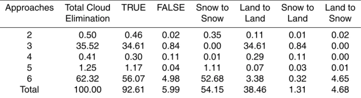
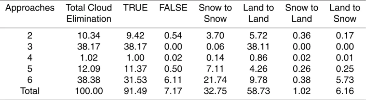
Interactive Discussion For example, on validation day 1 (Table 1), the approaches 3 and 6 performed the
best whereas the other approaches have almost negligible results. Apparently, most cloud coverage was on land covered pixels on that day since the performance from land to land is about 34%. On validation day 2 (Table 2), approaches 2 and 5 also perform reasonably well. Approach 2 is based on previous and next day information. 5
The performance was very low on validation day 1 because of dense cloud coverage from the previous and next days. Approach 4 generally performed more poorly but still was included as one of the approaches. Approach 5 performed differently and this also depends on the cloud coverage structure as it can be seen from both validation days. Approach 6 is based on the threshold dates for snow melt and snow accumulation. This 10
removes all clouds from the snow cover product. It can be seen from the validation that it is acceptable to use this method to remove the clouds, but one should also be aware that this approach has most of the error as it was about 6% for the validation day 1 and validation day 2. Nevertheless, it is more acceptable to have about 5% cloud coverage error than having almost 62% of the entire basin being covered by clouds 15
(validation day 1). This performance also changes from day to day as it can be seen from validation results. An improvement to the results could be carried out through the adjustment of finding the threshold date for each pixel, but this was not carried out in this study and is an outlook for future work.
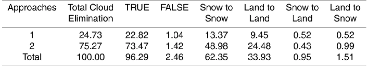
Additionally, performances of individual approaches were also tested. The combi-20
nation of Terra and Aqua products (approach 1) was kept in each individual validation since the performance of this approach is assumed to be the best among others. The other individual approaches were included after approach 1. The results are given in Table 4 where the Julian day 33 (2 February) was taken as an example.
In the Table 4, all possible cloud elimination is taken and among them 24.7% of the 25
cloud was eliminated using the approach 1and 75.3% of the cloud was eliminated using the approach 2. As seen, both approaches performed with little error (FALSE values).
HESSD
6, 791–841, 2009
Snow cover data (MODIS) for water balance applications
A. Gafurov and A. B ´ardossy
Title Page Abstract Introduction Conclusions References Tables Figures ◭ ◮ ◭ ◮ Back Close
Full Screen / Esc
Printer-friendly Version
Interactive Discussion shows that very high pixels in the catchment area were not covered by cloud on this
day.
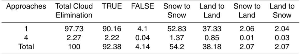
The same as approach 3, the approach 4 also shows little improvement in elimi-nating cloud covers but the performance is acceptable to include this approach in the algorithm.
5
The approach 5 also performed well where more that 46% of the cloud on the Julian day of 33 was removed and more than 46% of it was correctly estimated as snow or land.
The approach 6 eliminates all clouds according to time series method. This approach resulted with most error to the algorithm. Nevertheless, the error amount is acceptable 10
when studying high mountainous and ungauged basins where no information at all is possible. Over 13% of total 88.6% cloud elimination was FALSE, but this is also due to the fact that only 2 approaches (1 and 6) where included in this validation. Including all 6 approaches will most probably decrease the error due to the additional improvements using other approaches.
15
7 Conclusions
The objective of this study was to remove cloud covered cells from original MODIS Terra and Aqua satellite snow cover products to obtain snow cover information in the Kokcha Basin where no such data is available locally. Different approaches were ap-plied to accomplish this work. The results show good performance and provide snow 20
information data for mountainous regions which is very important in water balance studies. Approaches 1 to 5 show very good performance whereas approach 6 results in large errors because of possible “in between” snowfalls after snowmelt which gives false information about the threshold melt day. On average, 30% cloud removal was performed using approaches 1 to 5 and the rest was eliminated using the approach 25
HESSD
6, 791–841, 2009
Snow cover data (MODIS) for water balance applications
A. Gafurov and A. B ´ardossy
Title Page Abstract Introduction Conclusions References Tables Figures ◭ ◮ ◭ ◮ Back Close
Full Screen / Esc
Printer-friendly Version
Interactive Discussion which can be used to estimate available water resources, a source that fills resources
of the region.
Especially in central Asian regions (including the Kokcha Basin), water resources are very important to the economy since agriculture is the main source for economic stability. In the last years, there has been an appearance of water conflict between 5
Kyrgyzstan, Tajikistan and Uzbekistan. Kyrgyzstan and Tajikistan want to fill up their reservoirs during the summer from the snow melt from the mountains in their region to produce energy in winter, whereas Uzbekistan located in downstream of the Syrdarya River and Amudarya River downstream of Kyrgyzstan and Tajikistan, respectively, has no other source to irrigate its agricultural fields in the summer. It was the case in the 10
past years that Kyrgyzstan had to release water from its reservoir in a large amount because of reservoir capacity and energy production and this happened when Uzbek-istan’s demand for water was not high. Knowing the available amount of snow could lead to better management of the reservoirs in such mountainous areas. With ob-tainable energy (temperature) for snowmelt, rough water balance estimations could be 15
conducted. The results of this study could be applied for such studies.
References
CAWATERinfo – Portal of Knowledge for Water and Environmental Issues in Central Asia, http: //www.cawater-info.net/index e.htm, 2006–2008.
Emre, T. A., Zuhal, A., Arda, S. A., Aynur, S., and ¨Unal, S. A.: Using MODIS snow cover maps 20
in modeling snowmelt runoffprocess in the eastern part of Turkey, Remote Sens. Environ., 97, 216–230, 2005.
Hall, D. K., Riggs, G. A., Salomonson, V. V., DiGirolamo, N. E., and Bayr, K. J.: MODIS snow-cover products, Remote Sens. Environ., 83, 181–194, 2002.
Klein A., Barnett A., and Lee S.: Evaluation of MODIS snow-cover products in the Upper Rio 25
Grande River Basin, Geophys. Res. Abstr., 5, 12420, 2003.
HESSD
6, 791–841, 2009
Snow cover data (MODIS) for water balance applications
A. Gafurov and A. B ´ardossy
Title Page
Abstract Introduction
Conclusions References
Tables Figures
◭ ◮
◭ ◮
Back Close
Full Screen / Esc
Printer-friendly Version
Interactive Discussion National Snow and Ice Data Center, http://nsidc.org/index.html, 2006–2008.
Parajka J. and Bl ¨oschl G.: Validation of MODIS snow-cover images over Austria, Hydrol. Earth Syst. Sc., 679–689, 2006.
Parajka J. and Bl ¨oschl G.: Spatio-temporal combination of MODIS images – potential for snow cover mapping, Water Resour. Res., 44, W03406, doi:10.1029/2007WR006204, 2008. 5
HESSD
6, 791–841, 2009
Snow cover data (MODIS) for water balance applications
A. Gafurov and A. B ´ardossy
Title Page
Abstract Introduction
Conclusions References
Tables Figures
◭ ◮
◭ ◮
Back Close
Full Screen / Esc
Printer-friendly Version
Interactive Discussion Table 1a.Contingency table for Terra and Aqua products in % for 7 March 2003.
(a) Day 66 AquaSnow AquaLand
HESSD
6, 791–841, 2009
Snow cover data (MODIS) for water balance applications
A. Gafurov and A. B ´ardossy
Title Page
Abstract Introduction
Conclusions References
Tables Figures
◭ ◮
◭ ◮
Back Close
Full Screen / Esc
Printer-friendly Version
Interactive Discussion Table 1b.Contingency table for Terra and Aqua products in % for 7 April 2003.
(b) Day 98 AquaSnow AquaLand
HESSD
6, 791–841, 2009
Snow cover data (MODIS) for water balance applications
A. Gafurov and A. B ´ardossy
Title Page
Abstract Introduction
Conclusions References
Tables Figures
◭ ◮
◭ ◮
Back Close
Full Screen / Esc
Printer-friendly Version
Interactive Discussion Table 2.Validation results for each approach in % for validation day 1.
Approaches Total Cloud TRUE FALSE Snow to Land to Snow to Land to
Elimination Snow Land Land Snow
2 0.50 0.46 0.02 0.35 0.11 0.01 0.02
3 35.52 34.61 0.84 0.00 34.61 0.84 0.00
4 0.41 0.30 0.11 0.01 0.29 0.11 0.00
5 1.25 1.17 0.04 1.11 0.07 0.03 0.01
6 62.32 56.07 4.98 52.68 3.38 0.32 4.65
HESSD
6, 791–841, 2009
Snow cover data (MODIS) for water balance applications
A. Gafurov and A. B ´ardossy
Title Page
Abstract Introduction
Conclusions References
Tables Figures
◭ ◮
◭ ◮
Back Close
Full Screen / Esc
Printer-friendly Version
Interactive Discussion Table 3.Validation results for each approach in % for validation day 2.
Approaches Total Cloud TRUE FALSE Snow to Land to Snow to Land to
Elimination Snow Land Land Snow
2 10.34 9.42 0.54 3.70 5.72 0.36 0.17
3 38.17 38.17 0.00 0.06 38.11 0.00 0.00
4 1.02 1.00 0.02 0.14 0.86 0.02 0.01
5 12.09 11.37 0.50 7.11 4.26 0.26 0.25
6 38.38 31.53 6.11 21.74 9.78 0.38 5.73
HESSD
6, 791–841, 2009
Snow cover data (MODIS) for water balance applications
A. Gafurov and A. B ´ardossy
Title Page
Abstract Introduction
Conclusions References
Tables Figures
◭ ◮
◭ ◮
Back Close
Full Screen / Esc
Printer-friendly Version
Interactive Discussion Table 4.Validation results for individual approaches of 1 and 2.
Approaches Total Cloud TRUE FALSE Snow to Land to Snow to Land to
Elimination Snow Land Land Snow
1 24.73 22.82 1.04 13.37 9.45 0.52 0.52
2 75.27 73.47 1.42 48.98 24.48 0.43 0.99
HESSD
6, 791–841, 2009
Snow cover data (MODIS) for water balance applications
A. Gafurov and A. B ´ardossy
Title Page
Abstract Introduction
Conclusions References
Tables Figures
◭ ◮
◭ ◮
Back Close
Full Screen / Esc
Printer-friendly Version
Interactive Discussion Table 5.Validation results for individual approaches of 1 and 3.
Approaches Total Cloud TRUE FALSE Snow to Land to Snow to Land to
Elimination Snow Land Land Snow
1 88.38 81.53 3.71 47.78 33.76 1.86 1.85
3 11.62 11.62 0.00 0.00 11.62 0.00 0.00
HESSD
6, 791–841, 2009
Snow cover data (MODIS) for water balance applications
A. Gafurov and A. B ´ardossy
Title Page
Abstract Introduction
Conclusions References
Tables Figures
◭ ◮
◭ ◮
Back Close
Full Screen / Esc
Printer-friendly Version
Interactive Discussion Table 6.Validation results for individual approaches of 1 and 4.
Approaches Total Cloud TRUE FALSE Snow to Land to Snow to Land to
Elimination Snow Land Land Snow
1 97.73 90.16 4.1 52.83 37.33 2.06 2.04
4 2.27 2.22 0.04 1.37 0.85 0.01 0.03
HESSD
6, 791–841, 2009
Snow cover data (MODIS) for water balance applications
A. Gafurov and A. B ´ardossy
Title Page
Abstract Introduction
Conclusions References
Tables Figures
◭ ◮
◭ ◮
Back Close
Full Screen / Esc
Printer-friendly Version
Interactive Discussion Table 7.Validation results for individual approaches of 1 and 5.
Approaches Total Cloud TRUE FALSE Snow to Land to Snow to Land to
Elimination Snow Land Land Snow
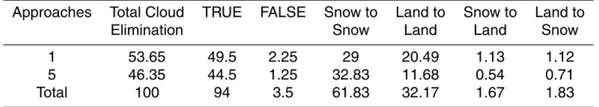
1 53.65 49.5 2.25 29 20.49 1.13 1.12
5 46.35 44.5 1.25 32.83 11.68 0.54 0.71
HESSD
6, 791–841, 2009
Snow cover data (MODIS) for water balance applications
A. Gafurov and A. B ´ardossy
Title Page
Abstract Introduction
Conclusions References
Tables Figures
◭ ◮
◭ ◮
Back Close
Full Screen / Esc
Printer-friendly Version
Interactive Discussion Table 8.Validation results for individual approaches of 1 and 6.
Approaches Total Cloud TRUE FALSE Snow to Land to Snow to Land to
Elimination Snow Land Land Snow
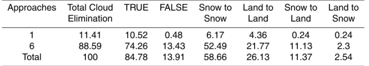
1 11.41 10.52 0.48 6.17 4.36 0.24 0.24
HESSD
6, 791–841, 2009
Snow cover data (MODIS) for water balance applications
A. Gafurov and A. B ´ardossy
Title Page
Abstract Introduction
Conclusions References
Tables Figures
◭ ◮
◭ ◮
Back Close
Full Screen / Esc
Printer-friendly Version
HESSD
6, 791–841, 2009
Snow cover data (MODIS) for water balance applications
A. Gafurov and A. B ´ardossy
Title Page
Abstract Introduction
Conclusions References
Tables Figures
◭ ◮
◭ ◮
Back Close
Full Screen / Esc
Printer-friendly Version
Interactive Discussion 0
20 40 60 80
1 2 3 4 5 6 7 8 9 10 11 12
Month
Pre
cipitation, Discha
100 120 140 160 180 200
rg
e (mm)
precipitation discharge
HESSD
6, 791–841, 2009
Snow cover data (MODIS) for water balance applications
A. Gafurov and A. B ´ardossy
Title Page
Abstract Introduction
Conclusions References
Tables Figures
◭ ◮
◭ ◮
Back Close
Full Screen / Esc
Printer-friendly Version
Interactive Discussion 0
50 100 150 200 250
1
19 37 55 73 91
109 127 145 163 181 199 217 235 253 271 289 307 325 343
Julian days
Pixel cover
Snow Land Snow
"complete snow
melt" "snow accumulation start"
snow (200)
cloud (50) land (25)
HESSD
6, 791–841, 2009
Snow cover data (MODIS) for water balance applications
A. Gafurov and A. B ´ardossy
Title Page
Abstract Introduction
Conclusions References
Tables Figures
◭ ◮
◭ ◮
Back Close
Full Screen / Esc
Printer-friendly Version
Interactive Discussion 0
50 100 150 200 250
1 17 33 49 65 81 97
113 129 145 161 177 193 209 225 241 257 273 289 305 321 337 353
Julian days
Pixel cover
Snow Land Snow
"complete snow melt"
"snow accumulation start"
snow (200)
cloud (50) land (25)
HESSD
6, 791–841, 2009
Snow cover data (MODIS) for water balance applications
A. Gafurov and A. B ´ardossy
Title Page
Abstract Introduction
Conclusions References
Tables Figures
◭ ◮
◭ ◮
Back Close
Full Screen / Esc
Printer-friendly Version
HESSD
6, 791–841, 2009
Snow cover data (MODIS) for water balance applications
A. Gafurov and A. B ´ardossy
Title Page
Abstract Introduction
Conclusions References
Tables Figures
◭ ◮
◭ ◮
Back Close
Full Screen / Esc
Printer-friendly Version
HESSD
6, 791–841, 2009
Snow cover data (MODIS) for water balance applications
A. Gafurov and A. B ´ardossy
Title Page
Abstract Introduction
Conclusions References
Tables Figures
◭ ◮
◭ ◮
Back Close
Full Screen / Esc
Printer-friendly Version
HESSD
6, 791–841, 2009
Snow cover data (MODIS) for water balance applications
A. Gafurov and A. B ´ardossy
Title Page
Abstract Introduction
Conclusions References
Tables Figures
◭ ◮
◭ ◮
Back Close
Full Screen / Esc
Printer-friendly Version
HESSD
6, 791–841, 2009
Snow cover data (MODIS) for water balance applications
A. Gafurov and A. B ´ardossy
Title Page
Abstract Introduction
Conclusions References
Tables Figures
◭ ◮
◭ ◮
Back Close
Full Screen / Esc
Printer-friendly Version
HESSD
6, 791–841, 2009
Snow cover data (MODIS) for water balance applications
A. Gafurov and A. B ´ardossy
Title Page
Abstract Introduction
Conclusions References
Tables Figures
◭ ◮
◭ ◮
Back Close
Full Screen / Esc
Printer-friendly Version
HESSD
6, 791–841, 2009
Snow cover data (MODIS) for water balance applications
A. Gafurov and A. B ´ardossy
Title Page
Abstract Introduction
Conclusions References
Tables Figures
◭ ◮
◭ ◮
Back Close
Full Screen / Esc
Printer-friendly Version
HESSD
6, 791–841, 2009
Snow cover data (MODIS) for water balance applications
A. Gafurov and A. B ´ardossy
Title Page
Abstract Introduction
Conclusions References
Tables Figures
◭ ◮
◭ ◮
Back Close
Full Screen / Esc
Printer-friendly Version
HESSD
6, 791–841, 2009
Snow cover data (MODIS) for water balance applications
A. Gafurov and A. B ´ardossy
Title Page
Abstract Introduction
Conclusions References
Tables Figures
◭ ◮
◭ ◮
Back Close
Full Screen / Esc
Printer-friendly Version
HESSD
6, 791–841, 2009
Snow cover data (MODIS) for water balance applications
A. Gafurov and A. B ´ardossy
Title Page
Abstract Introduction
Conclusions References
Tables Figures
◭ ◮
◭ ◮
Back Close
Full Screen / Esc
Printer-friendly Version
HESSD
6, 791–841, 2009
Snow cover data (MODIS) for water balance applications
A. Gafurov and A. B ´ardossy
Title Page
Abstract Introduction
Conclusions References
Tables Figures
◭ ◮
◭ ◮
Back Close
Full Screen / Esc
Printer-friendly Version
Interactive Discussion 0
20 40 60 80 100
Terra Aqua 1 2 3 4 5 6
Approaches
C
loud (%)
HESSD
6, 791–841, 2009
Snow cover data (MODIS) for water balance applications
A. Gafurov and A. B ´ardossy
Title Page
Abstract Introduction
Conclusions References
Tables Figures
◭ ◮
◭ ◮
Back Close
Full Screen / Esc
Printer-friendly Version
Interactive Discussion 0
20 40 60 80 0
Terra Aqua 1 2 3 4 5 6
Approaches
Cloud (%
)
10
HESSD
6, 791–841, 2009
Snow cover data (MODIS) for water balance applications
A. Gafurov and A. B ´ardossy
Title Page
Abstract Introduction
Conclusions References
Tables Figures
◭ ◮
◭ ◮
Back Close
Full Screen / Esc
Printer-friendly Version
Interactive Discussion
0 20 40 60 80 100
Terra Aqua 1 2 3 4 5
Approaches
Cloud (%)
HESSD
6, 791–841, 2009
Snow cover data (MODIS) for water balance applications
A. Gafurov and A. B ´ardossy
Title Page
Abstract Introduction
Conclusions References
Tables Figures
◭ ◮
◭ ◮
Back Close
Full Screen / Esc
Printer-friendly Version
Interactive Discussion 0
20 40 60 100
Terra Aqua 1 2 3 4 5 6
Approaches
C
loud (%
)
80
HESSD
6, 791–841, 2009
Snow cover data (MODIS) for water balance applications
A. Gafurov and A. B ´ardossy
Title Page
Abstract Introduction
Conclusions References
Tables Figures
◭ ◮
◭ ◮
Back Close
Full Screen / Esc
Printer-friendly Version
HESSD
6, 791–841, 2009
Snow cover data (MODIS) for water balance applications
A. Gafurov and A. B ´ardossy
Title Page
Abstract Introduction
Conclusions References
Tables Figures
◭ ◮
◭ ◮
Back Close
Full Screen / Esc
Printer-friendly Version
HESSD
6, 791–841, 2009
Snow cover data (MODIS) for water balance applications
A. Gafurov and A. B ´ardossy
Title Page
Abstract Introduction
Conclusions References
Tables Figures
◭ ◮
◭ ◮
Back Close
Full Screen / Esc
Printer-friendly Version
HESSD
6, 791–841, 2009
Snow cover data (MODIS) for water balance applications
A. Gafurov and A. B ´ardossy
Title Page
Abstract Introduction
Conclusions References
Tables Figures
◭ ◮
◭ ◮
Back Close
Full Screen / Esc
Printer-friendly Version
HESSD
6, 791–841, 2009
Snow cover data (MODIS) for water balance applications
A. Gafurov and A. B ´ardossy
Title Page
Abstract Introduction
Conclusions References
Tables Figures
◭ ◮
◭ ◮
Back Close
Full Screen / Esc
Printer-friendly Version
HESSD
6, 791–841, 2009
Snow cover data (MODIS) for water balance applications
A. Gafurov and A. B ´ardossy
Title Page
Abstract Introduction
Conclusions References
Tables Figures
◭ ◮
◭ ◮
Back Close
Full Screen / Esc
Printer-friendly Version
HESSD
6, 791–841, 2009
Snow cover data (MODIS) for water balance applications
A. Gafurov and A. B ´ardossy
Title Page
Abstract Introduction
Conclusions References
Tables Figures
◭ ◮
◭ ◮
Back Close
Full Screen / Esc
Printer-friendly Version
Interactive Discussion Fig. 16. Comparison of Terra original and processed (after approach 5 and approach 6) data