www.geosci-model-dev.net/8/2611/2015/ doi:10.5194/gmd-8-2611-2015
© Author(s) 2015. CC Attribution 3.0 License.
MEMLS3&a: Microwave Emission Model of Layered Snowpacks
adapted to include backscattering
M. Proksch1,5, C. Mätzler2,6, A. Wiesmann2, J. Lemmetyinen3, M. Schwank2,4, H. Löwe1, and M. Schneebeli1 1WSL Institute for Snow and Avalanche Research SLF, Flüelastrasse 11, 7260 Davos Dorf, Switzerland
2GAMMA Remote Sensing Research and Consulting AG, Worbstrasse 225, 3073 Gümlingen, Switzerland 3Arctic Research Center, Finnish Meteorological Institute FMI, 00101 Helsinki, Finland
4Swiss Federal Institute for Forest, Snow and Landscape Research WSL, Zürcherstrasse 111, 8903 Birmensdorf, Switzerland 5Institute of Meteorology and Geophysics, University of Innsbruck, Innrain 52, 6020 Innsbruck, Austria
6Institute of Applied Physics, University of Bern, Sidlerstrasse 5, 3012 Bern, Switzerland
Correspondence to:M. Proksch ([email protected])
Received: 19 December 2014 – Published in Geosci. Model Dev. Discuss.: 6 March 2015 Revised: 27 July 2015 – Accepted: 8 August 2015 – Published: 24 August 2015
Abstract. The Microwave Emission Model of Layered Snowpacks (MEMLS) was originally developed for mi-crowave emissions of snowpacks in the frequency range 5–100 GHz. It is based on six-flux theory to describe ra-diative transfer in snow including absorption, multiple vol-ume scattering, radiation trapping due to internal reflec-tion and a combinareflec-tion of coherent and incoherent super-position of reflections between horizontal layer interfaces. Here we introduce MEMLS3&a, an extension of MEMLS, which includes a backscatter model for active microwave remote sensing of snow. The reflectivity is decomposed into diffuse and specular components. Slight undulations of the snow surface are taken into account. The treatment of like- and cross-polarization is accomplished by an empiri-cal splitting parameterq. MEMLS3&a (as well as MEMLS) is set up in a way that snow input parameters can be de-rived by objective measurement methods which avoid fit-ting procedures of the scattering efficiency of snow, required by several other models. For the validation of the model we have used a combination of active and passive mea-surements from the NoSREx (Nordic Snow Radar Experi-ment) campaign in Sodankylä, Finland. We find a reason-able agreement between the measurements and simulations, subject to uncertainties in hitherto unmeasured input param-eters of the backscatter model. The model is written in Mat-lab and the code is publicly avaiMat-lable for download through the following website: http://www.iapmw.unibe.ch/research/ projects/snowtools/memls.html.
1 Introduction
Empirical observations reveal a wide range of different mi-crowave signatures in active or passive remote sensing over snow covered areas as shown e.g., by Mätzler (1987). The lack of realistic models to understand these signatures was the motivation for efforts leading to the Microwave Emis-sion Model of Layered Snowpacks (MEMLS) in the 1990s (Mätzler, 1996; Wiesmann and Mätzler, 1999). Initially the microwave emission behavior of single snow layers was in-vestigated by Weise (1996) and later by Wiesmann (1997). The measurements led to an empirical approach for the scat-tering coefficient of snow in the frequency range 5–100 GHz and correlation-length range 0.05–0.3 mm (Wiesmann et al., 1998) as well as to a first version of MEMLS (Wiesmann and Mätzler, 1999). Empirical relations for the scattering co-efficient have also been implemented in the Helsinki Uni-versity of Technology (HUT) model developed by Pulliainen et al. (1999) and later adapted by Lemmetyinen et al. (2010). MEMLS was extended to coarse-grained snow for correla-tion lengths up to 0.6 mm (Mätzler and Wiesmann, 1999). The snow microstructure was characterized by an exponen-tial correlation function which allows computing the scatter-ing coefficient analytically usscatter-ing the improved Born approx-imation (IBA) (Mätzler, 1998).
can be measured directly and objectively by various meth-ods. Other models may require e.g., a conversion of mea-sured parameters to model-effective ones (Kontu and Pulli-ainen, 2010; Lemmetyinen et al., 2015). The exponential cor-relation length could be e.g., obtained by micro-computed to-mography (µCT) (Schneebeli and Sokratov, 2004) from a fit to the reconstructed three-dimensional microstructure (Löwe et al., 2013). Snow density and correlation length can be also obtained efficiently from field measurements (Proksch et al., 2015) using high-resolution penetrometry (SnowMicroPen – SMP) (Schneebeli and Johnson, 1998). Alternatively, optical methods can be used, e.g., Matzl and Schneebeli (2006); Gal-let et al. (2009); Arnaud et al. (2011), to measure the specific surface area (SSA) and use an empirical relation to compute the exponential correlation length (Mätzler, 2002). The latter method is appealing since SSA is commonly available. Ac-cordingly, MEMLS was widely used for various questions related to passive microwave remote sensing (Durand et al., 2008; Rees et al., 2010; Toure et al., 2011; Langlois et al., 2012; Schwank et al., 2014).
In recent years, there was an increasing interest of the snow remote sensing community in active microwave mea-surements, which was mainly driven by the Cold Regions Hydrology High-Resolution Observatory CoReH2O (Rott et al., 2010) and related activities. However, single-layer models for the radar signal as presented in Rott et al. (2010) or Ulaby et al. (1984) are mainly used for efficient opera-tion in retrieval schemes. For the sake of low complexity, these models are naturally based on strongly simplifying as-sumptions, e.g., treating snow as a collection of independent scatterers. However, scatterers are densely packed in snow and strongly interact with each other. More realistic models based on dense media radiative transfer (DMRT) have been developed (Tsang et al., 2007; Chang et al., 2014), including the possibility of using the numerical solution of Maxwell’s equations for the single-layer scattering coefficients (Ding et al., 2010; Xu et al., 2012). The DMRT-based models how-ever require at least two microstructural input parameters, which can be presently obtained only byµCT and often re-quire time consuming casting procedures in the field.
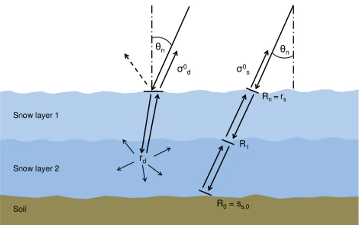
To cope with recent requirements in active microwave remote sensing, while relying on an established, physical model of intermediate complexity, it is the aim of the present paper to extend MEMLS and develop a first version of MEMLS3&a. Thereby, we can build on the description of the microstructure in terms of the exponential correlation length as a single, objective parameter which can be derived from in situ field measurements. For the backscattering model, we shall extend the description of the snowpack in MEMLS to account for a slightly undulated snow surface as shown in Fig. 1. The slightly undulated patches should be small enough to leave the emission largely unaffected but large enough to allow for specular backscattering at near-vertical incidence.
Snow layer 1
Snow layer 2
Soil
θn
θn
σ0 s
σ0 d
rd
Rn =rs
R1
R0 = ss,0
Figure 1.Snowpack (blue) with slightly undulated snow surface
and layers. Waves incident at nadir angleθn are refracted at the
snow surface followed by volume scattering with backscatterσd0 (left). Specular backscatterσs0from a slightly tilted patch of the surface, soil and layer interfaces (right). Diffuserd and specular
reflectivitiesrs=Rn,R0andR1are indicated.
The paper is organized as follows: in Sect. 2 we present the development of the model and the calculation of the to-tal backscatter with its specular and diffuse components. In Sect. 3 the validation data consisting of active and passive microwave measurements from Sodankylä, Finland, are de-scribed. Section 4 presents the validation of both MEMLS and MEMLS3&a using the Sodankylä data, followed by a discussion (Sect. 5) and the conclusions (Sect. 6). Details about the calculation of the specular reflectivity are given in the Appendix.
2 Model development
Since the total reflectivity of a snowpack is related to its emissivity, it can be derived from passive observations alone. Thereby, active and passive observables can be appropriately combined to obtain a prediction for the radar backscatter. 2.1 Link between active and passive observables At any given frequency and polarization of electromagnetic radiation with incident direction(µn, φn)defined by zenith angle θn (where µn=cosθn) and azimuth angle φn at the snow–air interface (cf. Fig. 1), the reflectivityrof the surface is related to its emissivity e(in the reciprocal direction) by Kirchhoff’s law:
r=1−e . (1)
For a more general description of Kirchhoff’s law, see Mät-zler and Melsheimer (2006). Equation (1) relates the emissiv-ity, the key quantity of passive microwaves, to the reflectivemissiv-ity, a quantity linked to scattering. It is this relation that allows us to link active and passive microwave remote sensing. The re-flectivity represents the fraction of the incident radiation that is scattered in the hemisphere above the surface. If the scat-tered radiation is diffuse (Lambertian reflectance) we can es-timate the fraction in the backscatter direction. Furthermore, with information about the statistics of surface slopes, we can determine the contribution of backscatter arising from specu-lar reflection at surface facets that are normal to the incident direction. Therefore, we will represent the total reflectivity as a sum of diffuse and specular components. The reflectiv-ity can be represented as an integral over scattering directions in the upper hemisphere of the bistatic scattering functionS:
r= 1
4π µn Z
2π
S(µn, φn, µ, φ)d= 1 2µn
1 Z
0
S(µn, µ).dµ (2)
Here, d=dµdφ is the infinitesimal solid-angle element in the scattered direction. The azimuth integration extends from 0 to 2π, and the last expression is valid for azimuth-independent functions. The function S describes the scat-tering from incident direction (µn, φn) to the scattering direction (µ, φ). Thus, backscattering is determined by
S(µn, φn, µn, φn). Chandrasekhar (1960) introduced the S function in his monograph on radiative transfer. He showed thatSis reciprocal:
S(µn, φn, µ, φ)=S(µ, φ, µn, φn). (3) Furthermore, S is identical to the bistatic scattering cross section σ0 introduced by Ulaby et al. (1981), see their Eqs. (4.186) and (4.187), more exactly to the sum of the like- and cross-polarization terms, S=σlike0 (θn, φn, θ, φ)+ σcross0 (θn, φn, θ, φ). It is also related to Peake’s (1959) func-tionγ=S/µn; i.e., the 1/µnfactor of Eq. (2) is included in-side this function. For completeness, we note thatSis related
to but differs from other definitions: the reflection functionR
used for instance by Kokhanovsky (2001) differs by a fac-torπ from the bidirectional reflection distribution function (BRDF) used in optical remote sensing (Kasten and Raschke, 1974), and all quantities are related by
S(µn, φn, µ, φ)=µnγ (µn, φn, µ, φ)
=4µnµ R(µn, φn, µ, φ)
=4π µnµBRDF(µn, φn, µ, φ). (4) TheSfunction can be highly complex. However, for diffuse scattering, some empirical functions are provided in the liter-ature, see e.g., Mätzler and Rosenkranz (2007), the simplest one for Lambert scattering:
Sd=S0µnµ, (5)
where the subscript d indicates diffuse scattering, andS0is a constant. By integration according to Eq. (2), we find that the diffuse reflectivityrdis independent of the incidence an-gle, namelyrd=S0/4=R, and thus equal to Kokhanovsky’s
R. The normalized backscattering cross section is given by
σd0=Sd(µ=µd), which can be expressed byrdvia
σd0=4rdµ2n. (6)
Indeed, Lambertian behavior was found by the investigation of the HPACK model for snow by Mätzler (2000). It is an extension of an earlier one-layer, active–passive model of Tsang et al. (1982) to include multiple-isotropic scattering in the snow as well as refraction and reflection at the snow surface. The combined effect led to Lambert scattering for the diffuse component.
Unspecified in Eq. (6) is the separation of σd0 in its like- and cross-polarized components. For isotropic scatter-ers considered in HPACK, the first-order backscattering is like-polarized, and cross-polarization requires higher-order scattering. However, the structure of natural snow is highly complex, meaning that cross-polarization occurs for all scat-tering orders. Therefore, we introduce an empirical relation-ship with a splitting parameterq which defines the cross-polarized part, whereas(1−q)represents the like-polarized fraction, via
σd0,pp′=
(1−q)σd,v0 , p=p′=v
(1−q)σd,h0 , p=p′=h
qσd,v0 +σd,h0 /2, p=v, p′=h orp=h, p′=v.
(7)
polariza-tion, respectively:
σd,v0 =σd,vv0 +σd,hv0 =4rd,vµ2n,
σd,h0 =σd,hh0 +σd,vh0 =4rd,hµ2n. (8) An additional contribution to backscattering results from specular reflection as shown in Fig. 1. By considering only slight undulations, specular backscattering is limited to near-vertical incidence. For a Gaussian distribution of surface slopes, the backscattering coefficient of the specular term can be written as
σs0=rs,0 exp
−tan2θn/(2m2) 2m2µ4
n
, (9)
wherem2 is the mean-square slope, andrs,0 refers tors at normal incidence (Fig. 1, right). This equation corresponds to the geometrical-optics solution for undulating surfaces, see Ulaby et al. (1982, Eqs. 12.45 and 12.46), and Kong (1986, Sect. 6.6). Here we generalize it from surface scattering to specular terms that fit the observation geometry (i.e., spec-ular reflectivity for local normal incidence angle). Further-more, we note that Eq. (9) describes like-polarized backscat-ter. For negligible anisotropy in the local surface plane the same values are obtained for hh (horizontal) and vv (verti-cal) polarization, and the cross-polarization terms are zero.
For both v and h polarization the total reflectivity is the sum of the diffuse and the specular component:
r=rd+rs. (10)
While Eqs. (6) and (8) are valid forrd, Eq. (9) applies tors but taken at normal incidence. With some additional effort described below, MEMLS provides both rd andrs and the total backscattering coefficient as the sum:
σ0=σd0+σs0. (11)
2.2 Determination ofr
Apart from the physical temperatures of all snow layers in-cluding the ground temperature, the downwelling sky bright-ness temperature Tsky must also be provided as input in MEMLS. The output is the brightness temperature Tb that is observed as upwelling radiation above the snowpack
Tb=rTsky+(1−r)Teff. (12)
HereTeff is the emission-effective temperature of snow and ground. The reflectivityrcan thus be computed viaTb(Tb1,
Tb2) from two arbitrary and different values ofTsky (Tsky1,
Tsky2), such as 100 and 0 K. The reflectivity then follows from
r= Tb1−Tb2 Tsky1−Tsky2
. (13)
2.3 Determination ofrs
According to Fig. 1 we need the specular reflectivities rs,v andrs,hat vertical and horizontal polarization at the observa-tion incidence angle as well asrs,0at normal incidence. For brevity, we omit subscripts indicating the polarization and just writersinstead ofrs,vandrs,h. In many situationsrscan be identified by the reflectivity of the snow surface. This is especially true for wet snow and for snowpacks that consist of a single layer. However, if an old snowpack is covered by fresh snow, the dominant specular layer may be the in-terface between the fresh and the old snow. Also, ice lenses form dominant reflectors inside the snowpack. Therefore, MEMLS requires a method that estimates incoherent spec-ular reflectivities for arbitrary stratifications. This derivation is detailed in the Appendix. As a result, if all layer interfaces are assumed to be smooth and the corresponding interface reflectivitiessj are determined by Fresnel’s equations, the specular reflectivityRj resulting from layers belowzj can be expressed in terms of a recurrence relation
Rj=sj+
[(1−sj)uj]2Rj−1 1−u2jsjRj−1
, j=1, . . ., n. (14)
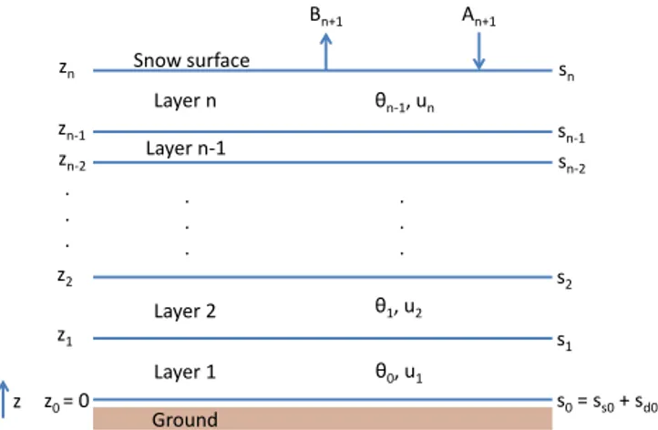
wheresj is the interface reflectivity on top of layer j and uj=exp(−γe,jdj/µj−1)is the coherent transmissivity of layerj (Fig. 2). The extinction coefficient is denoted byγe,j anddj is the layer thickness. The specular reflectivity of the entire snowpack–ground system then is given by
rs=Rn (15)
Equation (14) starts withj=1 at the ground as the lowest layer contributing to specular reflection. In contrast to the smooth interfaces assumed between snow layers, the ground is regarded as a rough surface and its reflectivity is addi-tively decomposed into a diffuse and a specular part accord-ing tos0=ss,0+sd,0. Accordingly, the ground reflectivity R0=ss,0constitutes the initial condition for the recurrence relation (14).
2.4 Synopsis of the backscatter model
Finally, we briefly recap how specular and diffuse compo-nents from the previous section are practically reassembled in MEMLS3&a for the computation of the total backscatter.
1. The total backscatterσ0is divided into a specular and diffuse component,σs0andσd0, respectively (cf. Eq. 11). 2. The specular componentσs0is derived from Eq. (9) and arises from the rough soil surface (viass,0) and the layer interfaces and the snow–air interface, both of which are assumed to be slightly undulated.
Ground Snow surface
Layer n
Layer n-1
Layer 2
Layer 1 . . . .
. .
sn
sn-1 sn-2
s1 s2
s0 = ss0 + sd0 An+1
Bn+1
zn
zn-1 zn-2
z1 z2
z0 = 0
. . .
θ1, u2
θ0, u1 θn-1, un
z
Figure 2.Geometry of then-layered snowpack with up- and
down-welling intensitiesAandB. Heightzj, transmissivityujof directed
radiation, refracted angleθj−1and interface reflectivitysjfor layer
numberjranging from 1 (bottom) ton(top). Snow–ground reflec-tivitys0, consisting of the specularss0and diffuse componentsd0.
reflectivity r (Eq. 13) and its specular component rs (Eqs. 14, 15).
Thus, the model accounts for multiple scattering at the un-dulated layer interfaces. The diffuse scattered radiation is as-sumed to be Lambertian, which allows estimating the frac-tion scattered in the backscatter direcfrac-tion. More complex processes such as coherent backscatter enhancement recently presented by Tan et al. (2015) are currently not considered in MEMLS3&a.
2.5 Primary input parameters
For a simulation run at a given frequencyf, polarizationp
and observation incidence angleθn, all snow physical param-eters described in Table 1 are required for each snow layer (j =1,2, . . ., n). From these primary input parameters, sec-ondary parameters are computed as described in the previous version of MEMLS (Wiesmann and Mätzler, 1999).
3 Validation data
We used snow input data generated from three different snow measurement methods to run model simulations which are compared to backscatter measurements from ESA’s SnowS-cat sSnowS-catterometer for validation (Werner et al., 2010). All measurements were made on 1 March 2012 at the test site of the Finnish Meteorological Institute (FMI), in Sodankylä, Finland, during ESA’s Nordic Snow and Radar Experiment (NoSREx) III (Lemmetyinen et al., 2013). The snow mea-surements were conducted directly in the field of view of the scatterometer and the radiometer in order to minimize the in-fluence of the spatial variability of the snowpack.
3.1 Test site
In the NoSREx campaign, the SnowScat scatterometer and SodRad radiometers were installed on two platforms over-looking a forest clearing. For the NoSREx measurements, SnowScat was set to measure several incidence angles over a wide sector. For the purpose of the present work both SnowScat and SodRad were turned in azimuth to point to-wards the same location on the snowpack, where a destruc-tive snow-pit measurement was made after the microwave measurements were completed.
The soil composition under the snowpack is dominantly mineral soil, with a thin vegetation layer on the surface (ca. 5 cm). A survey conducted in 2010 resulted in a soil compo-sition beneath the vegetation layer of 70 % sand, 1 % clay and 29 % silt. Trees and shrubs higher than 10 cm were removed from the site prior to measurements. The surface vegetation consists of low lichen, moss and heather (Fig. 14).
3.2 SnowScat
The validation data were measured with ESA’s SnowScat in-strument (Werner et al., 2010) developed by Gamma remote sensing, Gümlingen, Switzerland. It is an X-to-Ku band, fully polarimetric step-frequency radar with an internal cal-ibration loop which measures at a frequency range of 9.2– 17.8 GHz, with a frequency resolution of 3.072 MHz. Data are presented for three sub-bands with center frequencies of 10.2, 13.3 and 16.7 GHz with 2 GHz bandwidth. The−3 dB beam widths of the horn antennas are 5 and 12◦, depending
on frequency and polarization. An aluminum sphere is used as calibration target to correct for long-term drifts. The in-strument is mounted on a 9 m high tower and is able to rotate in the azimuth direction and to vary the incidence angle. For the validation data used in this study, SnowScat was pointed directly at the location where the in situ measurements were conducted. The instrument was then operated at an incidence angle of 50◦.
3.3 SodRad
Table 1.Primary input parameters used in MEMLS3&a, with snow input parameters for each snow layer (upper part) and general model parameters (lower part). In addition, the value and unit of the parameter, as well as a typical way of determination, are indicated.
Parameter Value and unit Determination
densityρ [0–917] kg m−3 traditionala, SMP, CT
exponential correlation lengthlex mm SMP, CT, (NIP)b
volume fraction of liquid water [0–1] traditionala, dielectricc
snow salinity [0–0.1] ppt electric conductivity
layer thickness cm traditionala, SMP, NIP, CT
temperatureT K traditionala
physical ground temperatureT0 K thermometer
snow–ground reflectivitys0 [0–1] modeledd
specular snow–ground reflectivityss0 [0–1] estimated froms0e
cross-polarization ratioq [0–1] empirical
mean slope of surface undulationsm [0–∞] empirical
aFierz et al. (2009).bIn combination with a density measurement (Eqs. 16, 17).cDenoth et al. (1984).
dWegmüller and Mätzler (1999).dSee text, Sect. 4.1.2.
4 Validation results 4.1 Model initialization 4.1.1 Snow input parameters
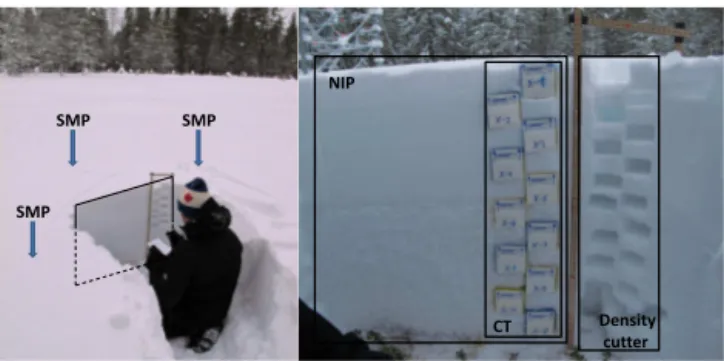
The most crucial snow input parameters required to drive MEMLS3&a are density and correlation length. We derived these parameters from three different snow measurement methods in order to illustrate different ways of acquisition (Fig. 3). First, density and correlation length were derived ac-cording to Löwe et al. (2011), using three-dimensional recon-struction byµCT (Schneebeli and Sokratov, 2004) of snow samples cast in the field. The sample casting technique is de-scribed in detail by Heggli et al. (2009). Second, we used the SMP (Schneebeli and Johnson, 1998), a high resolution pen-etrometer. The derivation of density and correlation length from the SMP is detailed in Proksch et al. (2015). Finally, the near-infrared photography (NIP) developed by Matzl and Schneebeli (2006) allows measuring the specific surface area (SSA) of snow which is used to define the length scale:
lc=
4(1−ρsnow/ρice)
SSA . (16)
The exponential correlation lengthlexis then obtained from the empirical relation,
lex=0.75lc, (17)
put forward by Mätzler (2002).
As NIP does not provide the snow density, it was mea-sured using a standard 100 cm3density cutter with a vertical sampling interval of 4 cm. A more detailed comparison of snow measurement methods with respect to microwave re-mote sensing can be found in Proksch and Schneebeli (2012). The density and correlation length profiles derived by the
NIP
CT Density
cutter SMP
SMP
SMP
Figure 3. Left: snow-pit overview with the locations of the
SnowMicroPen (SMP) measurements (arrows) surrounding the pro-file wall (black rectangular). Right: close-up of the propro-file wall, with locations of near infrared photography (NIP), computed tomogra-phy (CT) and density cutter measurements.
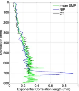
different methods are shown in Figs. 4 and 5. In general, the different methods are in agreement, besides the correla-tion length derived from NIP, which shows very large values in the lowest layer, an artifact of the preparation process of the profile wall. The snow temperature was assumed to be constant at−3◦C. At this temperature the snow is dry and
does not contain liquid water. The density and correlation length profiles were averaged to a vertical resolution of 3 cm to avoid any effects of coherent layers for the wavelength considered by SnowScat.
4.1.2 Soil contribution
Figure 4.Density profile derived by SMP (green),µCT (black) and density cutter (blue). The green line is the average of three neigh-boring SMP measurements.
Takala et al., 2011; Rautiainen et al., 2012; Kontu et al., 2014). We used a value for the complex soil permittivity of frozen ground ofǫg=3.6+0.9i, in line with Rautiainen et al. (2012), and set the standard deviation of the soil surface height rmsgunder the vegetation to 5 mm.
To account for the correct incidence angle at the snow– ground interface, the following auxiliary procedure is carried out for each model run. First, MEMLS3&a is run withs0=0 and the incidence angle at the snow–ground interface is de-termined. Second, this angle was used in the model of Weg-müller and Mätzler (1999) to calculate s0 which was then used to run MEMLS3&a again, now accounting for the cor-rect incidence angle on the snow–ground interface. The re-sulting values fors0ranged from 0.025 for 18 GHz at v-pol to 0.037 for 10 GHz at h-pol.
The model of Wegmüller and Mätzler (1999) gives the to-tal reflectivity of the snow–ground interface. To determine its specular componentss0, we assumedss0to be proportional to
s0. A constant factor of 0.75 (ss0=0.75s0, for all polariza-tions and frequencies) was chosen to match SnowScat mea-surements with our simulations.
The soil temperature was measured to be−2.5◦C. For the comparison to SnowScat observations, the cross-polarization fraction q was chosen to match the microwave measure-ments, which led toq=0.15. The mean slope of surface un-dulationsmhas no influence for an incidence angle of 50◦if values are smaller than 0.25. We choosem=0.1 for our sim-ulations. The sensitivity to both parameters will be discussed in Sect. 4.2.2.
Figure 5.Correlation length profile derived by SMP (green),µCT
(black) and NIP (blue). The blue line is the correlation length de-rived from the SSA measured by NIP according to Mätzler (2002).
4.1.3 Sky temperature
A further input to the model is the downwelling brightness temperatureTsky of the sky. As SnowScat did not measure
Tsky, we estimatedTskyfrom the SodRad radiometer which measures the sky brightness temperatureTsky,zat zenith. To fit our frequency interval of 10–18 GHz used for the simula-tion, we linearly interpolatedTsky,zvalues to match the inter-val. To convertTsky,zto an effective sky brightness tempera-tureTsky, which is representative for the whole scenery at the main test site, we first determined the sky opacityτzat zenith fromTsky,z(similar to Mätzler, 1994, their Eq. 7):
τz= −ln T
sky,z−Tair
Tback−Tair
, (18)
whereTair=270 K is the air temperature andTback=2.7 K is the background radiation. A good approximation for the effective opacity (τeff) representative of the whole scenery is given by
τeff=2τz, (19)
as shown by Mätzler (2005). The sky brightness temperature is finally computed from
Tsky=2.7e−τeff+(1−e−τeff)Tair. (20)
4.2 Results
4.2.1 Simulation results
Figure 6. σ0 measured by SnowScat (circles) and modeled by MEMLS3&a (lines) with SMP (solid), CT (dashed) and NIP (dot-ted) inputs. MEMLS3&a runs are performed with the snow–ground reflectivity s0 calculated by Wegmüller and Mätzler (1999), and
ss0,h= 0.75s0,h,ss0,v= 0.75s0,v. The mean slope of the surface
undulation was set to m=0.1 and the cross-polarization ratio to q=0.15. Colors represent polarization, with vv – black, hh – blue and hv – red.
snow andTskyparameter settings described in Sect. 4.1, the results for MEMLS3&a driven by SMP, CT and NIP input data are shown in Fig. 6 for an incidence angle of 50◦. CT and SMP input results in good agreement between model and measurement, with mean absolute errors (MAEs) of 4.0×10⁻³and 4.3×10⁻³for vv polarization, 3.2×10⁻³and 1.6×10⁻³for hh polarization and 4.0×10⁻⁴and 5.3×10⁻⁴ for hv polarization with CT and SMP inputs, respectively. NIP input leads to an overestimation of σ0, which emerges from the NIP artefact towards the bottom of the profile (Sect. 4.1.1) where the correlation length values are too large. However, MEMLS3&a driven with CT input data is in good agreement with SnowScat measurements (Fig. 7).
The dependence on the incidence angle at 10.2 and 16.7 GHz is shown in Figs. 8 and 9. MEMLS3&a is in gen-eral agreement with SnowScat, with MEAs of 2.3×10⁻³ and 9.6×10⁻³for vv polarization, 2.1×10⁻³and 1.2×10⁻² for hh polarization and 6.3×10⁻⁴and 2.6×10⁻³for hv po-larization at 10.2 and 16.7 GHz, respectively. The polariza-tion difference is slightly too small at 16.7 GHz. The SnowS-cat observations at different incidence angles show a certain amount of scatter, which we attribute to the heterogeneity of the ground and snow cover at the test site.
4.2.2 Sensitivity analysis
In this section, the sensitivity of MEMLS3&a toss0as well as to the two empirical parameters, the cross-polarization ratio q and the root-mean-square slope of surface
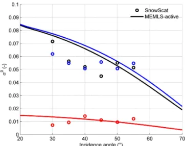
undula-Figure 7.σ0at incidence angle 50◦measured by SnowScat
(cir-cles) and modeled by MEMLS3&a with CT input (lines) for best fit parameters:ss0,h=0.75·s0,h;ss0,v=0.75·s0,v;q=0.15; and
m=0.1. Colors represent polarization, with vv – black, hh – blue and hv – red.
Figure 8.σ0at 10.2 GHz measured by SnowScat (circles) and
mod-eled by MEMLS3&a with CT input (lines). Colors represent polar-ization, with vv – black, hh – blue and hv – red. Best fit parameters according to Fig. 7.
tionsm, are shown. For clarity, we restrict ourselves to those MEMLS3&a runs which were driven with CT input data and the best fit values mentioned above (q=0.15,m=0.1, and
ss0=0.75s0 for both polarizations), if not indicated differ-ently.
Figure 9.σ0at 16.7 GHz measured by SnowScat (circles) and mod-eled by MEMLS3&a with CT input (lines). Colors represent polar-ization, with vv – black, hh – blue and hv – red. Best fit parameters according to Fig. 7.
significantly increased with decreasing ss0 values and vice versa, more pronounced at low frequencies.
The empirical cross-polarization ratio q is the frac-tion of cross-polarized backscatter: increasingq lowers co-polarization and increases cross-co-polarization by the same magnitude (cf. Eq. 7). Figure 11 illustrates this by two values ofq(0.15 and 0.3, respectively).
A larger value of mrepresents a stronger undulated sur-face and increases the spectral component of the backscatter, in particular at small incidence angles. Figure 12 shows this behavior, with increasing backscatter for increasing values ofmand decreasing incidence angles. Given values smaller than 0.1,mhas no effect at incidence angles larger than 25◦. Furthermore, cross-polarization is in general not affected by
m. Note that these results are only valid for the given snow and soil conditions, i.e., the sensitivity of parameters might change in different environmental conditions.
4.2.3 Comparison with passive simulations
To prove the concept of the MEMLS architecture, which is the fundament for MEMLS3&a, we compare our active sim-ulations with passive simsim-ulations using the same input data (Sect. 4.1). The validation data were measured by the So-dRad radiometer (Sect. 4.1.3). Similar to SnowScat, SoSo-dRad was also pointed to the location of the in situ measurements (azimuth angle 140◦). The instrument was operated at an in-cidence angle of 50◦.
To run MEMLS, 15 SMP measurements inside the main test site in Sodankylä were used in order to capture the spa-tial variability of the snowpack. For each SMP measurement one MEMLS simulation was conducted. Figure 13 shows the
Figure 10.σ0at incidence angle 50◦measured by SnowScat
(cir-cles) and modeled by MEMLS3&a with CT input (lines) for differ-ent specular snow–ground reflectivitiesss0. Higherss0values lead
to lowerσ0 values and vice versa. Colors represent polarization, with vv – black, hh – blue and hv – red. Best fit parameters accord-ing to Fig. 7.
Figure 11.σ0at incidence angle 50◦measured by SnowScat
(cir-cles) and modeled by MEMLS3&a with CT input (lines) for differ-ent cross-polarization ratiosq. Higherqratios lead to lowerσ0 val-ues for co-polarization and higherσ0values for cross-polarization. Colors represent polarization, with vv – black, hh – blue and hv – red. Best fit parameters according to Fig. 7.
results of the 15 MEMLS runs in combination with the So-dRad measurements.
ob-Figure 12. σ0 measured by SnowScat (circles) and modeled by MEMLS3&a with CT input (lines) at 10.65 GHz for different mean slope of surface undulationsm. Colors represent polarization, with vv – black, hh – blue and hv – red. Best fit parameters according to Fig. 7.
servation decreased to 16 and 1 K for v-pol and h-pol, respec-tively. The differences at 10 GHz are comparably lower, with 5 K at maximum. The standard deviations of the 15 MEMLS runs, which are solely due to spatial variability of the snow, increased with frequency. At 36 GHz, the standard deviation was around 8 K for both polarizations. The difference in az-imuth angles of SodRad was even larger, with 12 K at 36 GHz h-pol. This underlines the influence of the spatial variability of the snowpack on modeled and measured brightness tem-peratures, which will be discussed in the next section. The agreement between model and observation should be always interpreted with respect to the variation in brightness temper-atures caused by the spatial variability of the snowpack.
5 Discussion
As shown in Sect. 4, MEMLS3&a simulations were in rea-sonable agreement with SnowScat observations. To achieve this agreement, however, several parameters were chosen to match model and observation. This was necessary, since the active part contains, in contrast to the passive part, empiri-cal parameters (ss0, qandm) which could not be measured. Likewise, the ground parameterss0and rmsgare subject to uncertainties.
The specular part of the snow–ground reflectivityss0was chosen to be proportional tos0and the same factor of 0.75 could be applied for all frequencies and polarizations to con-verts0intoss0. Withss0=0.75s0, the main part of the snow– ground reflectivity is specular. This requires the ground to be smooth and the overlaying snow layer to be transparent. The vegetation is subject to very low temperatures and a steady
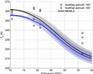
Figure 13.Tbmeasured by SodRad at an azimuth angles of 190◦
(circles) and at 140◦ (squares). Tb modeled by MEMLS from
15 SMP measurements, average (lines) with standard deviation (shaded). Colors represent polarization, with v – black and h – blue.
temperature gradient, which forces the water of the soft veg-etation (lichen, mosses, shrubs (myrtillus species); Fig. 14) to move upwards into the snow. Given the height of the veg-etation of less than 10 cm, it seems reasonable to assume that the vegetation dries out during winter and can be treated as fully transparent for the present microwave frequencies. This allows the soil interface to act as specular reflector, which is then accounted for byss0 in the model. Though being rea-sonable, a sound justification of this line of argumentation requires further investigations.
The cross-polarization in MEMLS3&a is solely deter-mined empirically via the parameter q. This pragmatic approach was chosen since the physical origin of cross-polarization in snow is still the subject of ongoing research. In the DMRT based approach (Tsang et al., 2007), cross-polarization emerges from non-spherical shapes of aggre-gated sphere clusters. A different route to cross-polarization can be taken via the discrete dipole approximation (DDA), e.g., from Von Lerber et al. (2006) or Xu et al. (2012), which principally accounts for multiple reflections and polariza-tions inside a given snow volume. DDA requires the full three-dimensional description of the microstructure, which can be provided by µCT. A comparison to such a model could further elucidate the justification and the value of the parameterq.
cor-Figure 14.View of about 1 m2of the snow-free surface at the ra-diometer test site in Sodankylä, Finland.
relation length of the height correlation function. According to Manes et al. (2008)mwould then take a value of 0.14 for fresh snow which is in the same order of magnitude as ap-plied in our simulations (m=0.1). This small-scale rough-ness of the snow surface is not taken into account by the model, where only slight surface undulations are allowed.
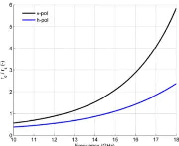
The individual magnitudes of the specular and diffuse con-tributions are shown in Fig. 15. Towards higher frequencies, the diffuse component increases and outweighs the specular reflectivity from 12.5 GHz for v-pol and from 14.5 GHz for h-pol. Note that the magnitude of the specular component also depends on the undulation of the surface and therefore on the value of m. However, a pronounced impact of mis limited to small incidence angles (Fig. 12 and Sect. 4.2.2) for reasonable values ofm(m≈0.1).
In contrast to MEMLS3&a, MEMLS does not require free empirical parameters. In this regard, we attribute the fact that MEMLS3&a matches the SnowScat observation better than MEMLS the SodRad observations to the additional free parameters in MEMLS3&a, foremost ss0 and q. However, for the passive simulations, parameters also had to be cho-sen without direct experimental justification, namely s0and rmsg, which determine the contribution of the snow–ground interface. This contribution is dominant and critical in our frequency range, as dry snowpacks thinner than ∼1 m are highly transparent. Unfortunately, the knowledge about the scattering at the ground surface is limited. Therefore, the snow–ground reflectivity s0 was modeled using the model of Wegmüller and Mätzler (1999). This model is an empiri-cal parametrization of the Fresnel formula depending on the standard deviation of the soil surface height rmsgand the soil permittivities. For the soil permittivities, Hallikainen et al. (1985) provide experimental data and Mironov et al. (2010) an empirical model based on experimental data, but dielec-tric models for the permittivities of frozen soils are still un-der development. For rmsg of the soil below the snowpack no measurements were available. In addition, the model of
Figure 15.Ratio of the simulated diffuse (rd) and specular (rs)
re-flectivity at 50◦incidence angle per frequency, for the best fit pa-rameters according to Fig. 7.
Wegmüller and Mätzler (1999) does not account for veg-etation, which is in our case consistent with the argument on transparency given above. We note that estimating the snow–ground reflectivity is critical for all microwave mod-els, which was also concluded from recent experiments (Roy et al., 2013; Montpetit et al., 2013). However, at 10 GHz, the frequency which is most influenced by the soil; MEMLS and SodRad were in good agreement.
In contrast, the mismatch between model and measure-ments was largest at 36 GHz and is most sensitive to details of the snow microstructure. MEMLS assumes an exponen-tial fit of the density correlation function of the snow mi-crostructure. The exponential fit is a reasonable starting point but small deviations can have a large influence on scattering. As detailed by Löwe et al. (2011), the correlation function of snow can take different shapes and its representation by means of a single correlation length might be inappropriate. Instead the Teubner–Strey form, a two-scale form for bicon-tinuous media might be more appropriate. The inclusion of other types of correlation functions into MEMLS is possible by adapting the calculation of the scattering coefficient. We thus believe that the present model provides a suitable test case to investigate the impact of more sophisticated repre-sentations of the snow microstructure.
We further tried to assess the influence of the spatial vari-ability of the snowpack. The standard deviation obtained from the 15 MEMLS runs is 8 K at 36.5 GHz, h- and v-pol, implying a non-negligible influence of the location of the in situ snow measurements on the modeled brightness temper-atures.
environ-ment, such as trees, which were closer to the field of view at this azimuth angle. The spatial variability of the snowpack together with the influence of the environment is potentially able to bias simulated and measured brightness temperatures. The degree of complexity of existing models simulat-ing microwave backscattersimulat-ing from snow range from ssimulat-ingle- single-layer approaches (Rott et al., 2010) to numerical solutions of Maxwell’s equations (Xu et al., 2012; Ding et al., 2010). In this context, we propose MEMLS3&a as a model of interme-diate complexity. In contrast to the HUT model (Pulliainen et al., 1999; Lemmetyinen et al., 2010), which has compara-ble complexity, MEMLS avoids traditional grain size as in-put parameter, which is prone to uncertainties in the visual estimation method (Painter et al., 2007). The advantage of MEMLS3&a (as well as MEMLS) is the correlation length as microstructural quantity, which can be obtained from ob-jective measurements without conversion and, given the SMP retrieval method, with high efficiency in the field.
Presently, models differ not only in the representation of snow microstructure but also in the solution of the radiative transfer or the type of interfaces between the layers, which makes it difficult to attribute the discrepancies in model per-formance to a particular part of the model. A comparison by Tedesco and Kim (2006) of at least the passive models showed that no model was able to reproduce all of the inves-tigated microwave observations. For a detailed model assess-ment in view of future developassess-ments, various effects (spa-tial variability, snow microstructure, soil) must be isolated. A promising way is by using measurements of specifically prepared snow slabs, as already presented by Wiesmann et al. (1998). Together with complete 3-D microstructural infor-mation, these types of idealized experiments will allow us to
minimize spatial variability, avoid the influence of the ground and compare different microstructural concepts for scattering coefficients. Together with available multi-layer models like MEMLS3&a, ML (Picard et al., 2013) or the DMRT-QMS package (Chang et al., 2014), this will clarify our un-derstanding of the processes involved in microwave emission and scattering of snow.
6 Conclusions
We adapted the MEMLS to include backscattering and pre-sented a detailed description of the relevant parameters and their derivation. The reflectivity was decomposed into dif-fuse and specular components, and the snowpack was al-lowed to be slightly undulated. This procedure could be ap-plied to other passive microwave models as well. Model simulations were in reasonable agreement with scatterome-ter observations, if the specular snow–ground reflectivityss0 and the cross-polarization ratioq were chosen accordingly. We found that the contribution of the snow–ground inter-face is a critical parameter, which needs further investiga-tion. The empirical formulation of the cross-polarization ra-tioq is a limitation with respect to other existing microwave models. MEMLS3&a is a model of intermediate complexity, which avoids fitting procedures of the scattering efficiency of snow in combination with SMP orµCT measurements. This eliminates a main uncertainty of snow characterization in microwave remote sensing.
Appendix A: Specular reflectivity of the layered snowpack
The purpose of the appendix is to derive the specular part of the reflectivity of a layered snowpack, in order to separate it from the diffuse part by subtraction from the total reflectivity using MEMLS. It is assumed here that all layer interfaces are smooth and parallel to the surface in order to produce specular reflection. Separation between diffuse and specular reflection is required in bistatic scattering and in backscatter models.
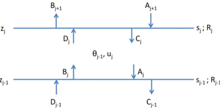
We consider a plane-parallel snowpack used in MEMLS as shown in Fig. 2. The relevant quantities of an arbitrary layerj are shown in detail in Fig. A1. The layer is specified by a transmissivityuj for the directed radiation. The trans-missivity is given by
uj=exp(−γe,jdj/cosθj−1), (A1) wheredj =zj−zj−1is the thickness andγe,jis the extinc-tion coefficient of layerj, respectively. In addition, the layer interfaces are characterized by an interface reflectivity, where
sj denotes the reflectivity of the top interface of layerj. As-suming smooth interfaces, we can apply the Fresnel formulas to computesj. The propagation angleθj−1in layerjis given by Snell’s law of refraction. At the bottom of the snowpack, the reflectivity s0=ss0+sd0 consists of a specularss0 and a diffusesd0component.
The aim of the following procedure is to derive an expres-sion for the total specular reflectivity,Rj, which results from transmission and reflections in all layers belowzj. In order to compute the specular reflectivity we assume sufficiently large directional intensities such that thermal radiation can be neglected. Note thatAj,Bj,CjandDjare downwelling and upwelling intensities just above and below the boundaries of the respective snow layer. By virtue of Fig. A1 we can derive the following equations relating the directional intensities at the boundaries:
Aj =ujCj, (A2)
Bj=Rj−1Aj, (A3)
Cj=(1−sj)Aj+1+sjDj, (A4)
Dj =ujBj, (A5)
Bj+1=RjAj+1=(1−sj)Dj+sjAj+1. (A6) Furthermore, at the bottom we have
R0=ss0, (A7)
wheress0 is the specular part of the ground-snow interface reflectivity.
In order to solve these equations forRj, we first eliminate theDj andCj in Eqs. (A4) and (A6) by using Eqs. (A2) and (A5). In this way we obtain
uj(1−sj)Aj+1=Aj−u2jsjBj, (A8)
sj ; Rj
sj-1 ; Rj-1
Aj+1
Bj+1
zj
zj-1
θj-1, uj
Dj-1
Dj
Cj-1
Cj
Aj
Bj
Figure A1.The parameters of a selected layerj: heightzj, up- and
downwelling intensitiesA, B, C, andD; transmissivityuj of
di-rected radiation; refracted angleθj−1; interface reflectivitysj; and
specular reflectivityRj.
and
Bj+1=(1−sj)ujBj+sjAj+1. (A9) Dividing Eq. (A8) byAj and Eq. (A9) byAj+1we get, to-gether with Eqs. (A6) and (A3),
uj(1−sj)Aj+1/Aj=1−u2jsjRj−1, (A10) and
Rj=(1−sj)ujRj−1Aj/Aj+1+sj. (A11) Eliminating the ratio Aj+1/Aj=(1−uj2sjRj−1)/[uj(1− sj)]in Eq. (A11) leads to
Rj=sj+
(1−sj)uj 2
Rj−1 .
1−u2jsjRj−1
. (A12) Equation (A12) is a recurrence relation for the total specular reflectivity at the snow surface,rs=Rn. The initial condition for the recurrence relation is given by the ground reflectivity in Eq. (A7).
The described procedure is applied for horizontal and ver-tical polarization, separately. For v polarization we callRn= rs,v, and for h polarization we callRn=rs,h. These are the specular parts of the total reflectivities,rvandrhof MEMLS. The diffuse componentsrd,vandrd,hare thus
rd,v=rv−rs,v,
rd,h=rh−rs,h. (A13)
Code availability
The model is written in Matlab and available to the public through the following website: http://www.iapmw.unibe.ch/ research/projects/snowtools/memls.html.
Acknowledgements. The validation data were acquired during Nordic Snow and Radar Experiment NoSREx III in Sodankylä, Finland, ESA ESTEC contract no. 22761/09/NL/JA. Proksch further acknowledges support from ESA’s Networking/Partnering Initiative NPI no. 235-2012. In particular we want to acknowledge FMI staff for help and support during the field campaigns. A first version of this model is based on ESA ESTEC contract no. 4200020716/07/NL/EL CCN2.
Edited by: N. Kirchner
References
Arnaud, L., Picard, G., Champollion, N., Domine, F., Gallet, J. C., Lefebvre, E., Fily, M., and Barnola, J. M.: Measurement of ver-tical profiles of snow specific surface area with a 1 cm resolution using infrared reflectance: instrument description and validation, J. Glaciol., 57, 17–29, doi:10.3189/002214311795306664, 2011. Chandrasekhar, S.: Radiative Transfer, Dover Publ., New York, NY,
1960.
Chang, W., Tan, S., Lemmetyinen, J., Tsang, L., Xu, X., and Yueh, S.: Dense media radiative transfer applied to SnowS-cat and SnowSAR, IEEE J. Sel. Top. Appl., 7, 3811–3825, doi:10.1109/JSTARS.2014.2343519, 2014.
Denoth, A., Foglar, A., Weiland, P., Mätzler, C., and Aebischer, H.: A comparative study of instruments for measuring the liq-uid water content of snow, J. Appl. Phys., 56, 2154–2160, doi:10.1063/1.334215, 1984.
Ding, K.-H., Xu, X., and Tsang, L.: Electromagnetic scattering by bicontinuous random microstructures with discrete permittivi-ties, IEEE T. Geosci. Remote, 48, 3139–3151, 2010.
Durand, M., Kim, E., and Margulis, S. A.: Quantifying uncertainty in modeling snow microwave radiance for a mountain snowpack at the point-scale, including stratigraphic effects, IEEE T. Geosci. Remote, 46, 1753–1767, doi:10.1109/TGRS.2008.916221, 2008. Fierz, C., Armstrong, R., Durand, Y., Etchevers, P., Greene, E., Mc-Clung, D., Nishimura, K., Satyawali, P., and Sokratov, S. A.: The international classification for seasonal snow on the ground, HP-VII Technical Documents in Hydrology 83, IACS Contribution 1, UNESCO-IHP, Paris, 2009.
Gallet, J.-C., Domine, F., Zender, C. S., and Picard, G.: Measument of the specific surface area of snow using infrared re-flectance in an integrating sphere at 1310 and 1550 nm, The Cryosphere, 3, 167–182, doi:10.5194/tc-3-167-2009, 2009. Hallikainen, M., Ulaby, F., Dobson, M., El-Rayes, M., and Wu, L.:
Microwave dielectric behavior of wet soil – Part 1: Empirical models and experimental observations, IEEE T. Geosci. Remote, 23, 25–34, 1985.
Heggli, M., Frei, E., and Schneebeli, M.: Instruments and methods snow replica method for three-dimensional
X-ray microtomographic imaging, J. Glaciol., 55, 631–639, doi:10.3189/002214309789470932, 2009.
Kasten, F. and Raschke, E.: Reflection and transmission terminol-ogy by analterminol-ogy with scattering, Appl. Optics, 13, 460–464, 1974. Kokhanovsky, A.: Optics of Light Scattering Media, Problems and
Solutions, 2nd Edn., Springer-Praxis, Chichester, UK, 2001. Kong, J. A.: Electromagnetic Wave Theory, John Wiley, New York,
1986.
Kontu, A. and Pulliainen, J.: Simulation of spaceborne microwave radiometer measurements of snow cover using in situ data and brightness temperature modeling, IEEE T. Geosci. Remote, 48, 1031–1044, doi:10.1109/TGRS.2009.2030499, 2010.
Kontu, A., Lemmetyinen, J., Pulliainen, J., Seppänen, J., and Hal-likainen, M.: Observation and modeling of the microwave bright-ness temperature of snow-covered frozen lakes and wetlands, IEEE T. Geosci. Remote, 52, 3275–3288, 2014.
Langlois, A., Royer, A., Derksen, C., Montpetit, B., Dupont, F., and Goïta, K.: Coupling the snow thermodynamic model SNOW-PACK with the microwave emission model of layered snowpacks for subarctic and arctic snow water equivalent retrievals, Water Resour. Res., 48, W12524, doi:10.1029/2012WR012133, 2012. Lemmetyinen, J., Pulliainen, J., Rees, A., Kontu, A., and
Derk-sen, C.: Multiple-layer adaptation of HUT snow emission model: comparison with experimental data, IEEE T. Geosci. Remote, 48, 2781–2794, doi:10.1109/TGRS.2010.2041357, 2010.
Lemmetyinen, J., Kontu, A., Leppänen, L., Pulliainen, J., Wies-mann, A., Werner, C., Proksch, M., and Schneebeli, M.: Tech-nical assistance for the development of an X- to Ku-Band Scat-terometer during the NoSREx III experiment, Final report, ESA ESTEC Contract No. 22671/09/NL/JA, European Space Agency ESA ESTEC, Noordwijk, the Netherlands, 2013.
Lemmetyinen, J., Derksen, C., Toose, P., Proksch, M., Pulliainen, J., Kontu, A., Rautiainen, K., Seppänen, J., and Hallikainen, M.: Simulating seasonally and spatially varying snow cover bright-ness temperature using HUT snow emission model and retrieval of a microwave effective grain size, Remote Sens. Environ., 156, 71–95, 2015.
Löwe, H., Egli, L., Bartlett, S., Guala, M., and Manes, C.: On the evolution of the snow surface during snowfall, Geophys. Res. Lett., 34, L21507, doi:10.1029/2007GL031637, 2007.
Löwe, H., Spiegel, J. K., and Schneebeli, M.: Interfacial and struc-tural relaxations of snow under isothermal conditions, J. Glaciol., 57, 499–510, doi:10.3189/002214311796905569, 2011. Löwe, H., Riche, F., and Schneebeli, M.: A general treatment
of snow microstructure exemplified by an improved rela-tion for thermal conductivity, The Cryosphere, 7, 1473–1480, doi:10.5194/tc-7-1473-2013, 2013.
Manes, C., Guala, M., Löwe, H., Bartlett, S., Egli, L., and Lehn-ing, M.: Statistical properties of fresh snow roughness, Water Resour. Res., 44, W11407, doi:10.1029/2007WR006689, 2008. Matzl, M. and Schneebeli, M.: Measuring specific surface area of
snow by near-infrared photography, J. Glaciol., 52, 558–564, doi:10.3189/172756506781828412, 2006.
Mätzler, C.: Applications of the interaction of microwaves with the seasonal snow cover, Remote Sens. Rev., 2, 259–387, 1987. Mätzler, C.: Microwave Transmissivity of a Forest Canopy:
Mätzler, C.: Microwave permittivity of dry snow, IEEE T. Geosci. Remote, 34, 573–581, doi:10.1109/36.485133, 1996.
Mätzler, C.: Improved Born approximation for scattering of ra-diation in a granular medium, J. Appl. Phys., 83, 6111, doi:10.1063/1.367496, 1998.
Mätzler, C.: HPACK, a bistatic radiative transfer model for mi-crowave emission and backscattering of snowpacks, and valida-tion by surface-based experiments, Tech. Rep. IAP research re-port 2000-4, University of Bern, Switzerland, 2000.
Mätzler, C.: Relation between grain-size and correlation length of snow, J. Glaciol., 48, 461–466, 2002.
Mätzler, C.: On the determination of surface emissivity from Satellite observations, IEEE Geosci. Remote S., 2, 160–163, doi:10.1109/LGRS.2004.842448, 2005.
Mätzler, C. and Melsheimer, C.: Radiative transfer and microwave radiometry, in: Thermal Microwave Radiation – Applications for Remote Sensing, ET Electromagnetic Waves Series 52, 1–23, Institution of Engineering and Technology (IET), London, UK, 2006.
Mätzler, C. and Rosenkranz, P.: Dependence of microwave bright-ness temperature on bistatic surface scattering: model functions and application to AMSU-A, IEEE T. Geosci. Remote, 45, 2130– 2138, 2007.
Mätzler, C. and Wiesmann, A.: Extension of the microwave emission model of layered snowpacks to coarse-grained snow, Remote Sens. Environ., 70, 317–325, doi:10.1016/S0034-4257(99)00047-4, 1999.
Mätzler, C. and Wiesmann, A.: Documentation for MEMLS, Ver-sion 3, Microwave EmisVer-sion Model of Layered Snowpacks, Tech. rep., Institute for Applied Physics, University of Bern, Switzerland, 2012.
Mironov, V., DeRoo, R., and Savin, I.: Temperature-dependable mi-crowave dielectric model for an Arctic soil, IEEE T. Geosci. Re-mote, 48, 2544–2556, 2010.
Montpetit, B., Royer, A., Roy, A., Langlois, A., and Derk-sen, C.: Snow microwave emission modeling of ice lenses within a snowpack using the microwave emission model for layered snowpacks, IEEE T. Geosci. Remote, 51, 4705–4717, doi:10.1109/TGRS.2013.2250509, 2013.
Painter, T., Molotch, N., Cassidy, M., Flanner, M., and Steffen, K.: Instruments and methods: contact spectroscopy for determina-tion of stratigraphy of snow optical grain size, J. Glaciol., 53, 121–127, doi:10.3189/172756507781833947, 2007.
Picard, G., Brucker, L., Roy, A., Dupont, F., Fily, M., Royer, A., and Harlow, C.: Simulation of the microwave emission of multi-layered snowpacks using the Dense Media Radiative transfer the-ory: the DMRT-ML model, Geosci. Model Dev., 6, 1061–1078, doi:10.5194/gmd-6-1061-2013, 2013.
Proksch, M. and Schneebeli, M.: Development of snow re-trieval algorithms for CoReH2O grain size estimator:
pro-cedures for objective snow pack structure parameters, Tech. Rep. 22830/09/NL/JC, European Space Agency, Noordwijk, the Netherlands, 2012.
Proksch, M., Löwe, H., and Schneebeli, M.: Density, specific surface area and correlation length of snow measured by high-resolution penetrometry, J. Geophys. Res., 120, 346–362, doi:10.1002/2014JF003266, 2015.
Pulliainen, J., Grandell, J., and Hallikainen, M.: HUT snow emission model and its applicability to snow water
equiv-alent retrieval, IEEE T. Geosci. Remote, 37, 1378–1390, doi:10.1109/36.763302, 1999.
Rautiainen, K., Lemmetyinen, J., Pulliainen, J., Vehviläinen, Dr-usch, M., Kontu, A., Kainulainen, J., and Seppänen, J.: L-band radiometer observations of soil processes in boreal and sub-arctic environments, IEEE T. Geosci. Remote, 50, 1483–1497, doi:10.1109/TGRS.2011.2167755, 2012.
Rees, A., Lemmetyinen, J., Derksen, C., Pulliainen, J., and En-glish, M.: Observed and modelled effects of ice lens for-mation on passive microwave brightness temperatures over snow covered tundra, Remote Sens. Environ., 114, 116–126, doi:10.1016/j.rse.2009.08.013, 2010.
Rott, H., Yueh, S., Cline, D., and Duguay, C.: Cold
re-gions hydrology high-resolution observatory for snow
and cold land processes, P. IEEE, 98, 752–765,
doi:10.1109/JPROC.2009.2038947, 2010.
Roy, A., Picard, G., Royer, A., Montpetit, B., Dupont, F., Langlois, A., Derksen, C., and Champollion, N.: Brightness temperature simulations of the Canadian seasonal snowpack driven by mea-surements of snow specific surface area, IEEE T. Geosci. Re-mote, 51, 4692–4704, doi:10.1109/TGRS.2012.2235842, 2013. Schneebeli, M. and Johnson, J.: A constant-speed penetrometer for
high-resolution snow stratigraphy, Ann. Glaciol., 26, 107–111, 1998.
Schneebeli, M. and Sokratov, S.: Tomography of tempera-ture gradient metamorphism of snow and associated changes in heat conductivity, Hydrol. Processes, 18, 3655–3665, doi:10.1002/hyp.5800, 2004.
Schwank, M., Rautiainen, K., Mätzler, C., Stähli, M., Lemmetyi-nen, J., PulliaiLemmetyi-nen, J., VehviläiLemmetyi-nen, J., Kontu, A., IkoLemmetyi-nen, J., Mé-nard, C. B., Drusch, M., Wiesmann, A., and Wegmüller, U.: Model for microwave emission of a snow-covered ground with focus on L band, Remote Sens. Environ., 154, 180–191, doi:10.1016/j.rse.2014.08.029, 2014.
Takala, M., Luojus, K., Pulliainen, J., Derksen, C., Lemmetyi-nen, J., Kämä, KoskiLemmetyi-nen, J., and Bojkov, B.: Estimating north-ern hemisphere snow water equivalent for climate research through assimilation of space-borne radiometer data and ground-based measurements, Remote Sens. Environ., 115, 3517–3529, doi:10.1016/j.rse.2011.08.014, 2011.
Tan, S., Chang, W., Tsang, L., Lemmetyinen, J., and Proksch, M.: Modeling both active and passive microwave remote sensing of snow using dense media radiative transfer (DMRT) theory with multiple scattering and backscattering enhancement, IEEE J. Sel. Top. Appl., in press, 2015.
Tedesco, M. and Kim, E.: Intercomparison of electromagnetic mod-els for passive microwave remote sensing of snow, IEEE T. Geosci. Remote, 44, 2654–2666, 2006.
Toure, A. M., Goïta, K., Royer, A., Kim, E. J., Durand, M., Mar-gulis, S. A., and Lu, H.: A case study of using a multilayered thermodynamical snow model for radiance assimilation, IEEE T. Geosci. Remote, 48, 2828–2837, 2011.
Tsang, L., Blanchard, A., Newton, R., and Kong, J. A.: A simple relation between active and passive microwave remote sensing measurements of earth terrain, IEEE T. Geosci. Remote, 20, 482– 485, 1982.
ra-diative transfer (DMRT) theory with multiple-scattering effects, IEEE T. Geosci. Remote, 45, 990–1004, 2007.
Ulaby, F., Moore, R., and Fung, A.: Microwave Remote Sensing Active and Passive, Vol. I, Microwave Remote Sensing Funda-mentals and Radiometry, Addison-Wesley Publishing Company, Reading, Mass., USA, 1981.
Ulaby, F., Moore, R., and Fung, A.: Microwave Remote Sensing Ac-tive and Passive, Vol. II, Radar Remote Sensing and Surface Scat-tering and Emission Theory, Addison-Wesley Publishing Com-pany, Reading, Mass., USA, 1982.
Ulaby, F., Stiles, W., and Abdelrazik, M.: Snow cover influence on backscattering from terrain, IEEE T. Geosci. Remote, 22, 126– 133, 1984.
Von Lerber, A., Sarvas, J., and Pulliainen, J.: Modeling snow volume backscatter combining the radiative transfer theory and the discrete dipole approximation, in: IEEE Interna-tional Conference on Geoscience and Remote Sensing, Sym-posium, 31 July–4 August 2006, Denver, CO, USA, 481–484, doi:10.1109/IGARSS.2006.128, 2006.
Wegmüller, U. and Mätzler, C.: Rough bare soil reflectivity model, IEEE T. Geosci. Remote, 37, 1391–1395, 1999.
Weise, T.: Radiometric and Structural Measurements of Snow, PhD thesis, Institute of Applied Physics, University of Bern, Switzer-land, 1996.
Werner, C., Wiesmann, A., Strozzi, T., Schneebeli, M., and Mät-zler, C.: The snowscat ground-based polarimetric scatterometer: calibration and initial measurements from Davos Switzerland, in: IEEE International Geoscience and Remote Sensing Symposium (IGARSS), 25–30 July 2010, Honolulu, HI, USA, 2363–2366, 2010.
Wiesmann, A.: Catalog of Radiometric and Structural snow sample measurements, Tech. Rep. IAP research report 97-1, University of Bern, Switzerland, 1997.
Wiesmann, A. and Mätzler, C.: Microwave emission model of layered snowpacks, Remote Sens. Environ., 70, 307–316, doi:10.1016/S0034-4257(99)00046-2, 1999.
Wiesmann, A., Mätzler, C., and Weise, T.: Radiometric and struc-tural measurements of snow samples, Radio Sci., 33, 273–289, 1998.
Xu, X., Tsang, L., and Yueh, S.: Electromagnetic models of co/cross polarization of bicontinuous/DMRT in radar remote sensing of terrestrial snow at X- and Ku-band for CoReH2O and SCLP