The Cryosphere, 7, 657–666, 2013 www.the-cryosphere.net/7/657/2013/ doi:10.5194/tc-7-657-2013
© Author(s) 2013. CC Attribution 3.0 License.
Geoscientiic
Geoscientiic
Geoscientiic
Geoscientiic
The Cryosphere
Open Access
Theoretical study of solar light reflectance from vertical snow
surfaces
O. V. Nikolaeva1and A. A. Kokhanovsky2
1Institute of Applied Mathematics, Miuuskaya Sq. 4, 125047, Moscow, Russia
2Institute of Environmental Physics, Bremen University, O. Hahn Allee 1, 28334 Bremen, Germany
Correspondence to:A. A. Kokhanovsky ([email protected])
Received: 27 July 2012 – Published in The Cryosphere Discuss.: 1 October 2012 Revised: 12 March 2013 – Accepted: 15 March 2013 – Published: 5 April 2013
Abstract.The influence of horizontal and vertical
inhomo-geneity of snow surfaces on solar light reflectance is studied using the radiative transfer theory (RTT). We compared 1-D RTT and 2-D RTT and found that large errors are produced if the 1-D RTT is used for the calculation of the snow re-flection function (and, therefore, also in the retrievals of the snow grain radii) in 2-D measurement geometries. Such 2-D geometries are common in the procedures for the determi-nation of the effective snow grain radii using near-infrared photography and spectroscopy of vertical snow walls. In par-ticular, we have considered three cases for the numerical cal-culations: (1) the case with no black film; (2) the case with a black film at the pit’s bottom; (3) the case with a black film at the pit’s bottom and also at one of the vertical snow walls.
1 Introduction
Optical measurements are commonly used to derive snow microphysical parameters from plane-parallel snow layers (Kokhanovsky et al., 2011). In particular, snow grain size is obtained from near-infrared (NIR) measurements (in the spectral range 865–1240 nm) of intensity of solar light re-flected from flat snow layers. The corresponding retrieval al-gorithms are based upon the physical phenomenon of the en-hancement of light absorption by larger ice grains (and as a consequence, a smaller light reflectance for snow layers with larger grains). The main problem with such a method is that only upper snow layers can be observed. The information on the snow microphysical parameters and snow pollution in deeper layers cannot be retrieved because of high absorp-tion of NIR radiaabsorp-tion by snow grains. As a matter of fact, NIR
radiation does not penetrate deep into a snowpack and, there-fore, does not contain information on the properties of snow from the depths above 1-5cm depending on the size of parti-cles and the wavelength (Kokhanovsky and Rozanov, 2012). To avoid this problem, recently measurements along vertical snow walls have become popular (see, e.g. Fig. 1 in Matzl and Schneebeli, 2006; and Fig. 2 in Painter et al., 2007). Also measurements along the length of cylindrical holes in snow are used (Barker and Korolev, 2010; Arnaud et al., 2011).
In most of cases (see e.g. Kokhanovsky et al., 2011) the 1-D transfer theory valid for plane-parallel slabs is used for the interpretation of optical measurements and determination of snow grain sizes. Although there could be some influ-ences of 3-D effects (e.g. shadowing from the snow walls, enhancement of brightness, etc.) on corresponding measure-ments. For the measurements involving 2-D and 3-D geome-tries (e.g. along snow walls), the approach based on the cor-relation of the reflectance and the snow grain size or the snow specific surface area (see e.g. Matzl and Schneebeli, 2006) is used. This is because more quantitative approaches based on the solution of radiative transfer equation in 2-D and 3-D ge-ometries have not been developed in applications relevant to optics of vertical snow walls.
658 O. V. Nikolaeva and A. A. Kokhanovsky: Theoretical study of solar light reflectance
0
H
snow
0
D H
snow snow
*
**
A
B Diffuse solar light source
X
C S
z
x y
air
R L O
P T
V
(R+X)/2
Fig. 1.The geometry of the problem.
The paper is structured as follows. In the next section we introduce the radiative transfer equation and boundary con-ditions relevant to the studies of light propagation in snow. The numerical algorithm developed for the solution of the corresponding integro-differential radiative transfer equation in the 2-D geometry is described in Sect. 3. The results of numerical experiments are reported in Sect. 4. The present study can be used to design and interpret real-world experi-ments relying on the spectrometry of vertical snow walls.
2 Radiative transfer equation and boundary conditions
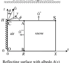
It is assumed that the surface of the snow is flat (no sastrugi, no microstructures on the snow surface). Let us assume that there is a pit with the widthD, the length Land the depth Hin the snowpack with the width 2Xand the heightH, see Fig. 1. The pit is covered by a sheer film to convert the di-rect solar light to diffuse one. Reflected radiation is registered along the line AB on the vertical wall of the pit and along the line CS at the top of the pit.
To find radiation intensity in this region, we introduce the coordinate system with the origin at the centre point O at the pit’s bottom, see Fig. 1. We assume that the length L (10–15 m) is larger than the typical widthD(about 1–3 m). Therefore, the radiation intensity near the central planey=0 of the pit depends only on the spatial coordinatesx andz. The dependence on the third coordinate can be neglected. So the problem can be considered in the 2-D framework in the planey=0. This reduces calculations as compared to the 3-D modelling. Moreover, the region is symmetrical with respect to the planex=0, see Fig. 1, hence only the half-region [0, X] × [0, H] instead of the region[−X, X] × [0, H] can be considered, see Fig. 2.
The radiative transfer equation (RTE) for the monochro-matic radiation intensityI takes the following form in the case under consideration:
∂I
∂ +σ (x, z) I (x, z, θ, ϕ) −σ (x, z) ω0(x, z)
π
Z
0
dθ′sinθ′
2π
Z
0
dϕ′ (1)
I (x, z, θ′, ϕ′) ρ(x, z, θ, ϕ, θ′, ϕ′)=0.
Reflecting surface with albedo
A
(
x
)
Diffuse solar light source
0
H
C
z
X
x
air
S
snow
*
R
A
B
**
y
O
0
Fig. 2.The 2-D half-region [0,X]× [0,H] with the wide rectan-gular pit [0,R]×[0,H] and the directionm{θ, φ}of the radiation transfer.
The functionI (x, z, θ, ϕ)depends on the spatial coordi-natesx, zand anglesθ,φ, defining directionof the radi-ation transfer, see Fig. 2. The first term in Eq. (1) gives the change of intensity in the directionand the second term represents the extinction of radiation by the medium. The in-tegral describes the re-radiation of scattered light, here inci-dent light has the direction ′(θ′, ϕ′)and re-radiated light has the direction(θ, ϕ).
The pit [0, R] × [0, H], R=D/2, is filled by air, whereas the medium out of the pit is snow. Then it follows that for the extinction coefficient:
σ (x, z) =
σair asx ≤R
σsnowasx > R , (2)
for the single scattering albedo:
ω0(x, z) =
ωair0 asx ≤R
ωsnow0 (z)asx > R , (3)
for the scattering phase function:
ρ(x, z, θ, ϕ, θ′, ϕ′) =
ρair asx ≤R
ρsnowasx > R. (4)
Note, the single scattering albedoωsnow0 (z)is considered as a piecewise function of depth, which describes a layered snowpack; the special caseωsnow0 (z)= const corresponds to a homogeneous snow layer.
O. V. Nikolaeva and A. A. Kokhanovsky: Theoretical study of solar light reflectance 659
0 H z
x y
0
X
Fig. 3.The 2-D region and directions of entering radiation.
with albedoA(x). Therefore, it follows that:
I (x,0, θ, ϕ)|0<θ <π/2 = A(x)
1 π
π Z
π/2
dθ′sinθ′ (5)
cosθ′
2π Z
0
dϕ′I (x,0, θ′, ϕ′).
Such a surface reflects incident radiation uniformly into all possible directions. If the bottom is covered by a black film absorbing all incident radiation, the albedoA(x)is made to be equal to zero and the bottom boundary is called “black”.
It is assumed that the radiation does not enter the region via the right boundaryx=X:
I (x, z, θ, ϕ)|π/2<ϕ<3π2 = 0. (6)
Reflecting condition with albedoAs is defined on the left boundaryx=0:
I (0, z, θ, ϕ)|0<ϕ<π/2∪3π /2<ϕ<2π (7) = AsI (0, z, θ, π−ϕ).
When As=1 Eq. (7) gives the condition of symme-try of the whole region[−X, X] × [0, H]with respect to the plane x=0. Actually, the solution of the RTE (Eq. 1) in the whole region [−X, X] × [0, H] is symmetrical: I (x, z, θ, ϕ) = I (−x, z, θ, π−ϕ). Therefore, one can con-sider the half-region [0, X] × [0, H]under the boundary condition (Eq. 7). WhenAs=0, the boundaryx=0 is black. It means that this boundary is covered by a black film absorb-ing all incident radiation.
The diffuse source on the top boundary is imposed. There-fore, it follows that:
I (x, H, θ, ϕ)|π/2<θ <π = S0
1
4π, (8)
whereS0is the incident light irradiance.
We will study three problems depending on albedo As at the left snow wall and the albedo A(x) at the bot-tom. First, under As=1, A(x)=Asnow>0 one has the pit with no black film. Second, under As=1, A(x) =
0 asx ≤R,
Asnow else, the black film lies only at the pit’s bot-tom. Third, underAs=0 and A(x) =
0 asx ≤R, Asnow else, the black film covers both the bottom and the vertical plane x=0.
Relative intensities of reflected radiation at the snow sur-face in the directions∗and∗∗:
˜
I (z) = I R, z,∗∗/S0, I (x)ˆ = I x, H,∗
/S0 (9)
are of interest. Here the functionI (x)ˆ defines the radiation intensity exiting from the top boundary in the zenith direc-tion∗. The functionI (z)˜ corresponds to radiation intensity reflected by the vertical wall AB of the snowpack (see Fig. 2) in the direction∗∗, perpendicular to the wall AB.
The functionI (x)ˆ can be used to retrieve the optical prop-erties of the upper layer of the snow (up to 5cm in depth). This function can be approximated by the piece-constant function:
b I (x) =
Iair(H,∗) asx ≤R Isnow(H,∗)asx > R,
where the valuesIsnow(H,∗)andIair(H,∗)are obtained via the two 1-D radiative transfer models as shown here (Chandrasekhar, 1950):
∂Isnow
∂ +σsnowIsnow(z, θ, ϕ)=σsnowωsnow0 (z)
π
R
0
dθ′
sinθ′
2Rπ
0
dϕ′Isnow(z, θ′, ϕ′) ρsnow(z, θ, ϕ, θ′, ϕ′)
, 0< z < H, (10)
∂Iair
∂ + σairIair(z, θ, ϕ) = σairω
air 0
π
R
0 dθ′
sinθ′
2Rπ
0
dϕ′Iair(z, θ′, ϕ′) ρair(θ, ϕ, θ′, ϕ′)
, 0< z < H. (11)
The boundary conditions are ( see the definition of angles in Fig. 3)
Isnow(H, θ, ϕ)|π/2<θ <π = 4Sπ0, Isnow(0, θ, ϕ)|0<θ <π/2
= Asnowπ π R
π/2
dθ′sinθ′ cosθ′
2π R
0
dϕ′Isnow(0, θ′, ϕ′),
Iair(H, θ, ϕ)|π/2<θ <π = S0
4π, I
air(0, θ, ϕ)| 0<θ <π/2
= Asnowπ π R
π/2
dθ′sinθ′ cosθ′
2Rπ
0
dϕ′Iair(0, θ′, ϕ′).
660 O. V. Nikolaeva and A. A. Kokhanovsky: Theoretical study of solar light reflectance
x y z
m m
m m
m
1 2
1 2
1 2,
m
1 2,
m
m, ,
(a) (b)
Fig. 4.An angular quadrature:(a)the node, (b)accommodation nodes of the quadrature.
Eq. (10) is solved along the line CO passing through the cen-tre of the pit, whereas the problem formulated in Eq. (11) is defined along the line TV passing through the centre of the snowpack, see Fig. 1.
The functionI (z)˜ is found by measuring light reflectance from snow walls and can be used to retrieve the optical and microphysical properties of the snow layers at any depth. This is not possible if, for example, the measurements of the light reflectance from the snow top (Kokhanovsky et al., 2011) are analysed. This is due to weak dependence of the snow reflectance in the UV and, also in the visible, on the size of particles and small penetration depths of IR radiation (sensitive to the snow microstructure) into snowpack. The re-trieval algorithms are based upon the assumption that the reg-istered radiation intensity is a constant function of the spatial coordinates in each homogeneous sub-region (layer) and this constant value does not depend on neighboring sub-regions (layers). It is actually believed that each sub-region (layer) of the snowpack can be considered separately from others. The constant valueI (z)˜ in each homogeneous layer is often believed equal to the valueIsnow(H,∗)for the homoge-neous snowpack under the same optical properties. Such an approach is “the horizontal 1-D transfer model”. The differ-ence of the 2-D solution and the 1D solutions is termed as “2-D effects”. We will check the accuracy of the 1D radia-tive transfer models using exact solutions of the 2-D problem (see Eqs. 1–8). We do not use the term “3-D effects” because the 2-D problem is under consideration.
3 Numerical algorithm
Below follows an outline of the numerical method used by us for the solution of the above radiative transfer problem. We introduce a quadrature with nodesm{θm, φm}, see Fig. 4a, and weights1m,m=1,. . . M. For this purpose we use the mesh over angleθ:
0< θ1/2 < θ3/2 < . . . < θℓ−1/2< θℓ+1/2 < θL+1/2=π
and the mesh over angleϕfor each intervalθℓ−1/2, θℓ+1//2
of the mesh overθ:
0< ϕ1/2, ℓ < ϕ3/2, ℓ < . . . < ϕn−1/2, ℓ< ϕn+1/2, ℓ < ϕNℓ+1/2, ℓ=2π.
’ ’
( , ,x z m, m, , )
Fig. 5.An adaptive angular quadrature to integrate a in the forward direction highly elongated phase function.
Points θℓ+1/2 and ϕn+1/2, ℓ have been chosen so that squares of all cells ϕn−1/2, ℓ, ϕn+1/2, ℓ
×θℓ−1/2, θℓ+1/2
are identical. We define the node{ϕnℓ, θℓ}in each cell, see
Fig. 4b, and renumber all nodes with a single indexm. Fur-ther we define the weight1mas a square of the correspond-ing cell1m.
Then we approximate the continuous function I (x, z, θ, φ) with functions Im(x, z)=I (x, z, θm, φm) and replace the scattering integral in Eq. (1) with the quadrature sum:
π
R
0
dθ′sinθ′
2π
R
0
dϕ′I (x, z, θ′, ϕ′) ρ(x, z, θm, ϕm, θ′, ϕ′)
∼ =
M
P
n=1
In(x, z) ρnm(x, z),
(12)
where ρnm(x, z)=
Z
1n
dϕ′dθ′ sinθ′ρ(x, z, θm, ϕm, θ′, ϕ′). (13)
The coefficients ρnm(x, z) correspond to the light scat-tering event from the direction n{θn, φn}to the direction m{θm, φm}. Therefore, they are the integrals of a compli-cated forward-peaked phase functionρ(x, z, θm, ϕm, θ′, ϕ′) over the cell1nunder fixed values of the angles{θm, ϕm}. To find the integral of a forward-peaked phase function one introduces the additional quadrature in the cell 1n by the nodesj, n{θj,n, ϕj, n}and the weights 1j, n,j = 1, . . . , Ln, hereLn is the number of the additional nodes. This quadrature is refined in the subregions of the cell1n, where the integrand function has a great gradient, see Fig. 5, where the additional nodesj, n{θj, n, ϕj, n}are designated by the black circles. The following equality is always kept:
Ln
X
j=1
1j, n = 1n. (14)
Then the coefficientρnm(x, z)can be found by a quadra-ture sum:
ρnm(x, z)= Ln
X
j=1
O. V. Nikolaeva and A. A. Kokhanovsky: Theoretical study of solar light reflectance 661
So Eq. (1) for the functionsIm(x, z)takes the form (with account for Eq. 10):
ξm∂Im/∂x+γm∂Im/∂z+σ (x, z) (1−ω0(x, z)ρmm(x, z)) Im(x, z)−σ (x, z) ω0(x, z)
M
P
n=1, n6=m
In(x, z) ρnm(x, z)=0 , (16) where the derivative∂∂I
m is written as: ∂I
∂m =
m,−→∇I
= ξm∂Im/∂x + γm∂Im/∂z. (17) The values
ξm = sinθmcosφm, γm = cosθm (18) are projections of the unit vectormonto coordinates axesx andz, see Fig. 4a.
To solve the system of differential equations (Eq. 16) for the functionsIm(x, z), we introduce a regular mesh over spa-tial variablesx,z:
0=x1/2 < ... < xk+1/2 < . . . < xK+1/2 = X, (19)
0=z1/2 < ... < zj+1/2 < ... < zJ+1/2 = H. (20)
Each cell [xk−1/2, xk+1/2] × [zj−1/2, zj+1/2] with steps
1xk = xk+1/2 −xk−1/2,1zj = zj+1/2 − zj−1/2is
con-sidered as a homogeneous one. Integrating Eq. (16) over this cell, one obtains the exact algebraic relation:
ξm(Im,k+1/2, j−Im, k−1/2, j)/1xk+γm(Im, k, j+1/2−Im, k, j−1/2)/
1zj +σk, j(1−ω0, k, jρmm, k, j)Im, k, j −σk, jω0, k, j M
P
n=1, n6=m
In, k, jρnm, k, j=0.
(21)
Here the valuesσk,j,ω0, k, j,ρnm, k, jcorrespond to the cell [xk−1/2, xk+1/2] × [zj−1/2, zj+1/2].
The values Im, k, j, Im, k±1/2, j, Im, k, j±1/2 are averaged
light intensities defined by the following integrals:
Im, k, j = 1 1xk1zj
xZk+1/2
xk−1/2
dx zjZ+1/2
zj−1/2
dz Im(x, z) (22)
Im, k±1/2, j = 1 1zj
zZj+1/2
zj−1/2
dz Im(xk±1/2, z) (23)
Im, k, j±1/2 =
1 1xk
xZk+1/2
xk−1/2
dx Im(x, zj±1/2). (24)
The boundary conditions for Eq. (19) follow from Eqs. (5–8):
Im, k, J+1/2
cosθm<0 =
1
4πS0, (25)
Im, k,1/2
cosθm>0=
Asnow
π
( X
cosθn<0
1n|cosθn|In, k,1/2
)
, (26)
Im,1/2, j
cosϕm>0= AsIn,1/2, j
cosϕn= −cosϕm, Im, K+1/2, j
cosϕm<0 =0.
(27)
To close Eqs. (19) and (23–25) one needs additional rela-tions. They are taken as
Im, k, j =(1−vm, k, j) Im, k+s(ξm)/2, j +vm, k, jIm, k−s(ξm)/2, j, (28)
Im, k, j =(1−um, k, j) Im, k, j+s(γm)/2+um, k, jIm, k, j−s(γm)/2, (29)
where the function s(ξ ) = sgn(ξ ) =
1 asξ >0,
−1 asξ <0 and the parameters vm, k, j, um, k, j are defined on the interval [0, 1]. Therefore, the piece-linear approximation to the so-lution is sought in the spatial cell, see Fig. 6. Here the pa-rametersvm, k, j,um, k, jdefine the variation of the solution in the cell (Carlson, 1972).
The resulting system of Eqs. (21) and (25–29) for the fixed nodem{θm, φm}consists of 3KJ+K+Jequations for the same number of unknowns. They are the values
Im, k+1/2,j, k=0, . . . , K, j=1, . . . , J, (30) Im, k, j+1/2, k=1, . . . , K, j=0, . . . , J,
Im, k, j, k=1, . . . , K, j =1, . . . , J.
Let the solution in the nodes n, n=1, . . . , m-1 and n=m+1, . . . Mbe known. Then the solution of the system (Eqs. 21 and 25–29) for the nodem can be found by the so-called sweep procedure in a following way.
Let the vectormbe defined by the angles from intervals 0< θm< π/2, 0< ϕm< π/2 when cosθm>0, cosϕm>0. The sweep procedure is the sequential computation of the valuesIm, k+1/2, j,Im, k, j+1/2 andIm, k, j under known val-uesIm, k−1/2, j,Im, k, j−1/2, as indeces increasek=1, . . . , K,
j=1, . . . , J. The obtained valuesIm, k+1/2,jandIm, k, j+1/2
are used to calculate the light intensity in the neighboring cells. Initial values on the left boundaryIm,1/2, jand the bot-tom boundaryIm, k,1/2are known due to the boundary
con-ditions (Eqs. 26 and 27).
If the anglesθm,ϕmare from other intervals, then indices are to be sorted in yet another order. Generally, the indexk increases ass(ξm) >0 and decreases ass(ξm) <0, the index j increases ass(γm) >0 and decreases ass(γm) <0.
662 O. V. Nikolaeva and A. A. Kokhanovsky: Theoretical study of solar light reflectance
x
1 2
k
x xk1 2
, 1 2,
m k j
I
, 1 2,
m k j
I
*
1 2 , ,
1 2(1 , , )
k m k j
k m k j
x x v
x v
Fig. 6.The piece-linear approximation to the RTE solution over the spatial variablexunderξm>0.
The relative intensities of reflected radiation at the snow surface in the directions ∗ and ∗∗ are sought. Direc-tions ∗(θ∗, φ∗)and∗∗(θ∗∗, φ∗∗)are defined by angles θ∗,φ∗andθ∗∗,φ∗∗, see Fig 2. They are not included in the quadrature nodes. To find the relative intensity in these direc-tions with no interpolation, two additional nodesM+1=
∗(θ∗, ϕ∗)andM+2=∗∗(θ∗∗, ϕ∗∗)with zero weights:
1M+1=1M+2=0 (31)
are inserted into the quadrature.
The previous version of the presented algorithm was out-lined by Sokoletsky et al. (2009), where it was applied to the calculation of solar light reflectance by natural sea wa-ters. There the scattering phase functions were defined by their values in nodes of a very refined mesh over the inter-val [−1, 1] and approximated by piecewise linear functions. Here the scattering phase functions are given by their Legen-dre coefficients. Furthermore, we apply the adaptive method of choosing additional meshesj, m to calculation of inte-grals (Eq. 15).
4 Results of numerical experiments
All computations were done by the code RADUGA-6 (Niko-laeva et al., 2005; Sokoletsky et al., 2009) on the hybrid clus-ter k100 (http://www.kiam.ru/MVS/resourses/k100.html) as-suming the following parameters:
1. the region height H=0.5 m, 0.6 m, 0.7 m, the region semi-widthX=5 m, see Fig. 1;
2. the pit widthD=0.4 m, 0.6 m, 0.8 m, 1 m, 2 m, 3 m, see Fig. 1;
3. the extinction coefficients σsnow=1 mm−1, σair= 0.001 mm−1;
4. the single scattering albedoωsnow0 (z)∈ [0.98,1],ωair0 = 1;
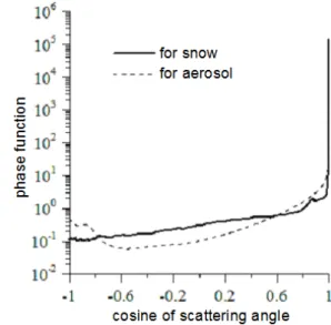
5. the air (aerosol) scattering phase function ρairis ob-tained via Mie theory, the snow phase functionρsnow (see Eq. 4) is found by geometrical optics theory as de-scribed by Kokhanovsky et al. (2011), see Fig. 7.
Fig. 7.The scattering phase functions. The molecular scattering is ignored and the air phase function is assumed to be equal to that of atmospheric aerosol.
6. snow albedoAsnow=0.8;
7. the diffuse source, when both a snowpack and a pit are covered by a sheer film.
We have selected a typical snow phase function as sug-gested by Kokhanovsky et al. (2011). The phase function does not depend strongly either on the wavelength (in the optical range) or on the size of ice grains. The extinction co-efficient 1 mm−1and the values of snow grain albedos in the range 0.98–1.0 are typical for snow.
Both homogeneous and heterogeneous snowpack were un-der consiun-deration. A homogeneous snowpack is defined by the constant single scattering albedoωsnow0 . A heterogeneous snowpack contains a polluted layer, see Fig. 8. It was as-sumed that:
ωsnow0 (z)=
0.98,as|z−h/2| ≤ t /2,
˜
ω0, as|z−h/2| > t /2. (32)
Here parameter t is thickness of a polluted layer, ω˜0 is
single scattering albedo of clean snow.
We define three experimental conditions (see Fig. 1): 1. no black film:As = 1,A(x)=Asnow=0.8;
2. a black film is only on the pit’s bottom EB:As = 1, A(x) =
0 asx ≤R, Asnow else ;
3. a black film is on the pit’s bottom EB and left boundary EC:As = 0,A(x) =
0 asx ≤R, Asnow else .
O. V. Nikolaeva and A. A. Kokhanovsky: Theoretical study of solar light reflectance 663
D H
air
snow snow
*
** A
B Diffuse solar light source
2X t
t
Fig. 8.The 3-D geometry of the region with the central polluted layer.
radiation intensity depends only on properties of the snow on the vertical wall AB. If there is no black film, one regis-ters the radiation reflected by both the bottom and two walls of the pit. Then the registered radiation depends on optical properties of the snow at all walls of the pit.
The following parameters are used in the numerical calcu-lations.
1. N=800 is the number of the Legendre polynomials to represent both phase functions;
2. M=360 is the number of nodes of the quadrature; one needs a dense quadrature to approximate the strongly anisotropic solutionI (x, z, θ, φ);
3. K=468,J=1610 are numbers of cells of the spatial meshes. The mesh overzis refined in the vicinity of the top boundary z=H, where the intensityI (x, z, θ, φ) has a large gradient. The mesh over x is refined near snowpack wall AB, see Fig. 2, for the same reason. Let us consider relative radiation intensityI (z)˜ given by Eq. (9) on the vertical wall AB of a snowpack, see Fig. 2, in the direction∗∗, which is perpendicular to the wall AB and at the top boundary CS of the system in the zenith direction ∗.
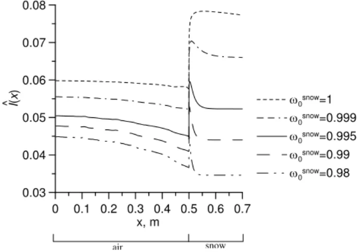
The relative intensity at the horizontal line CS in the zenith direction∗for homogeneous snowpack is given in Fig. 9. One can see that the intensity of reflected radiation has extrema near the air/snow boundary; similar effects are observed in clouds illuminated by direct solar light (Niko-laeva et al., 2005). In the problem under study a maximum of radiation intensity in the snow near the air/snow bound-ary is formed by radiation penetrating in the snowpack and only weakly absorbed near this boundary; the maximum en-hances as snow absorption enen-hances. In a similar way, a min-imum of radiation intensity arises outside of the snow near the air/snow boundary due to absorption of radiation by the snow. Thereby the extrema in the radiation intensity in Fig. 9 arise due to the neighbourhood of two different media (snow and air). Note the 1-D vertical transfer model leads to the
0 0.1 0.2 0.3 0.4 0.5 0.6 0.7 x, m
0.03 0.04 0.05 0.06 0.07 0.08
I
(
x
)
0snow=1
0snow=0.999
0snow=0.995
0snow=0.99
0snow=0.98
^
air snow
Fig. 9.Relative intensityI (x)ˆ in the zenith direction∗at the top boundary CS of the homogeneous snowpack. WidthD=1 m, depth
H=0.7 m and no black film, for the different single scattering albe-dosωsnow0 .
0 0.1 0.2 0.3 0.4 0.5 0.6 0.7
x, m 0.048
0.052 0.056 0.06 0.064 0.068 0.072
2D model 1D model
air snow
Fig. 10.Relative intensityI (x)ˆ in the zenith direction∗ on the top boundary CS of the homogeneous snowpack. WidthD=1 m, depthH=0.7 m, no black film, and the single scattering albedo
ωsnow0 =0.999, for the 2-D and 1-D models.
piecewise constant radiation intensity, see Fig. 10. Differ-ences between the 1-D and 2-D transfer models (2-D effects) reach 30 %.
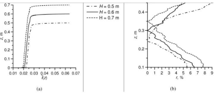
The calculated relative radiation intensityI (z)˜ at the ver-tical wall AB of a snowpack is presented in Figs. 11–15 for the various values of single scattering albedoωsnow0 , the depth H, the widthD=2Rand the surface albedosA(x)andAs. We introduce the functionr(z), defining the deviation of the functionI (z)˜ from its value in the central pointz=H/2:
r(z) = 100 h
1− ˜I (z)/I (H /˜ 2) i
0 0.02 0.04 0.06 I(z) 0 0.1 0.2 0.3 0.4 0.5 0.6 0.7 z , m ~ (a)
no black film black film on bottom black film on bottom and opposite side
0 20 40 60 80 100 120 r, % 0.05 0.1 0.15 0.2 0.25 0.3 0.35 0.4 0.45 0.5 0.55 0.6 0.65 z , m (b)
Fig. 11.Relative intensityI (z)˜ in the direction∗∗(a)and the de-viationr(z)(b)at the vertical wall AB of the homogeneous snow-pack. The snow single scattering albedoωsnow0 =0.98, the width
D=1 m, and depthH=0.7 m , with and without black film.
This deviation shows whether it is possible to consider the intensityI (z)˜ as a constant function far from the upper and lower boundaries of the pit. In other words it shows whether the 1-D model is applicable to process measurement data along vertical walls of snowpack.
It follows from Fig. 11 that the 1-D transfer model is not applicable for experiments under the black film because in this case the deviationr(z)is less than 10 % only near the central pointz=H /2. Actually, the size of the sub-region, where the deviationr(z)is less than 10 %, is equal to 7 cm – if both bottom and opposite sides are covered by the black film – and about 17 cm – if only the bottom is covered the black film. The size of this sub-region for the case without black film is about 55 cm.
The results for the pit without black film are shown in Figs. 12–15. It should be stressed that in this case the ra-diation registered on the wall AB is reflected by the bottom and the opposite walls of the pit and depends on the optical properties of the whole surface of the pit.
Let us consider homogeneous snowpack. Here the devia-tionr(z)decreases as absorption decreases (see Fig. 12) and the widthDof the pit increases (see Fig. 14). The function r(z)only weakly depends on the depthH(see Fig. 13).
At small values of the probability of photon absorption β=1−ω0 and in broad pit, the deviationr(z)is less than
the threshold value 10 % far from bottom and upper edges of the pit; here the 1-D model can be used. At the same time this deviation is large near the bottom and upper edges (boundary effects), where the 1-D model is not applicable.
The influence of heterogeneity of a snowpack on relative radiation intensity is presented in Figs. 12–15. The thin pol-luted layer in the centre of the pure snowpack, see Fig. 8, leads to a minimum in reflected radiation intensity in the vicinity of the layer (the shadow of the minimum is spread over the whole wall, if absorption in snow is weak enough). Let us define the width of the spread of the optical influence of the polluted layer as the size of the sub-region, where the relative intensity of the polluted layer differs more than by threshold valueb% from the relative intensity of the
homo-0 0.02 0.04 0.06 0.08
I(z) 0 0.1 0.2 0.3 0.4 0.5 0.6 0.7 z , m Layered snowpack t=5cm t=2cm t=1cm ~ 0 s n o w= 0 .9 8 0 s n o w= 0.9 9 0 snow=
1
5 cm 2 cm 1 cm
(a)
0 4 8 12 16 r, % 0.05 0.1 0.15 0.2 0.25 0.3 0.35 0.4 0.45 0.5 0.55 0.6 0.65 z, m
sn0
ow=1
0 snow
=1
0sno w=0.99
0sn ow=0.98
0 snow
=0.98
(b)
Fig. 12.Relative intensityI (z)˜ in the direction∗∗(a)and the de-viationr(z)(b)on the vertical wall AB of the heterogeneous snow-pack. Single scattering albedoω˜0=1 out of the inserted polluted
layer, widthD=1 m, depthH=0.7 m, and no black film, for the different values of the thicknesstof the inserted polluted layer.
0.01 0.02 0.03 0.04 0.05 0.06 0.07 I(z)
0 0.1 0.2 0.3 0.4 0.5 0.6 0.7 z , m ~ (a)
H = 0.5 m H = 0.6 m H = 0.7 m
0 1 2 3 4 5 6 7 8 9
r, % 0.1 0.2 0.3 0.4 z , m (b)
Fig. 13.Relative intensityI (z)˜ in the direction∗∗(a)and the de-viationr(z)(b)on the vertical wall AB of the homogeneous snow-pack. The snow single scattering albedoωsnow0 =0.98, the width
D=1 m, and no black film, for different depthsH.
geneous snowpack:
t∗(b) = minz − maxz (34)
|p(z)| < b%z > H /2 |p(z)|< b%, z < H /2. Here the pointz=H /2 is the central point of the whole snowpack and the polluted layer and the functionp(z)is de-fined by the relation:
p(z) = 100 h1− ˜I (z)/I˜0(z)
i
%. (35)
The functionI˜0(z)is the relative intensity in the
O. V. Nikolaeva and A. A. Kokhanovsky: Theoretical study of solar light reflectance 665
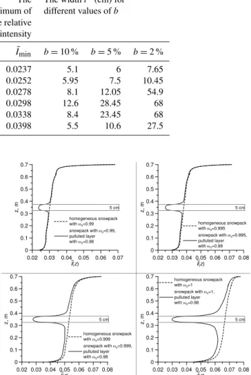
Table 1.The value of the minimum of the relative intensityI˜minand the width of the optical influence spread of the polluted layert∗(cm)
for different values of the single scattering albedoωsnow0 outside of the polluted layer at different widths of the polluted layert.
The single scattering The width of The The widtht∗(cm) for albedoωsnow0 out the polluted layer minimum of different values ofb
of the polluted layer t(cm) the relative intensity
˜
Imin b=10 % b=5 % b=2 %
0.99 5.0 0.0237 5.1 6 7.65
0.995 5.0 0.0252 5.95 7.5 10.45
0.999 5. 0 0.0278 8.1 12.05 54.9
1.0 5.0 0.0298 12.6 28.45 68
1.0 2.0 0.0338 8.4 23.45 68
1.0 1.0 0.0398 5.5 10.6 27.5
0 0.02 0.04 0.06 0.08 I(z)
0 0.1 0.2 0.3 0.4 0.5 0.6 0.7
z
, m
~
(a)
D = 0.4m D = 0.6m D = 0.8m D = 1m D = 2m D = 3m
0 10 20 30 40 50
r, % 0.05
0.1 0.15 0.2 0.25 0.3 0.35 0.4 0.45 0.5 0.55 0.6 0.65
z
, m
(b)
Fig. 14.Relative intensityI (z)˜ in the direction∗∗(a)and the de-viationr(z);(b)on the vertical wall AB of the homogeneous snow-pack. The snow single scattering albedoω0snow=0.98, the depth
H=0.7 m for, no black film, different widthsD.
layer depends on the width of this layer and the single scat-tering albedo outside of this layer, see Fig. 15 and Table 1. Note that the minimum decreases as the width of the layer decreases and the albedo of surrounding medium increases.
5 Conclusions
We have presented the 2-D radiative transfer problem re-lated to the reflection of solar light by a rectangular wide pit in a thick snow layer. Simulation (by the parallel code RADUGA-6) is based upon the mesh technique of the dis-crete ordinate method when peaked scattering phase func-tions of snow are exactly taken into account. A diffuse radi-ation source, produced by a sheer film covering a snowpack, is assumed. Such source models are close to those for real ground measurements.
We have checked whether the 1-D model, when the re-flected radiation intensity is considered as constant function of the spatial coordinate in each homogeneous subregion of a snowpack, is applicable to describe the real measurements.
0.02 0.03 0.04 0.05 0.06 0.07
I(z) 0
0.1 0.2 0.3 0.4 0.5 0.6 0.7
z, m
homogeneous snowpack
with 0=0.99
snowpack with 0=0.99,
pulluted layer
with 0=0.98
~
5 cm
0.02 0.03 0.04 0.05 0.06 0.07 0.08
I(z) 0
0.1 0.2 0.3 0.4 0.5 0.6 0.7
z, m
homogeneous snowpack
with 0=0.995
snowpack with 0=0.995,
pulluted layer
with 0=0.98
~
5 cm
0.02 0.03 0.04 0.05 0.06 0.07 0.08
I(z) 0
0.1 0.2 0.3 0.4 0.5 0.6 0.7
z, m
homogeneous snowpack
with 0=0.999
snowpack with 0=0.999,
pulluted layer
with 0=0.98
~
5 cm
0.02 0.03 0.04 0.05 0.06 0.07 0.08
I(z) 0
0.1 0.2 0.3 0.4 0.5 0.6 0.7
z, m
homogeneous snowpack
with 0=1
snowpack with 0=1,
pulluted layer
with 0=0.98
~
5 cm
Fig. 15.Relative intensityI (z)˜ in the direction∗∗on the verti-cal wall AB of the heterogeneous snowpack. WidthD=1 m, depth
H=0.7 m, thickness of the inserted polluted layert=5 cm, and no black film, for different values of the single scattering albedoω˜snow0
out of the inserted layer.
We found that the 2-D effects (brightening and shadowing) on the top boundary of a snowpack near the vertical wall of the pit are significant in spite of a diffuse radiation source.
The 2-D effects are significant on the vertical wall of the pit in a homogeneous snowpack, especially near the upper boundary. At the same time, 2-D effects are less evident at large values of the pit’s width far from its bottom and top boundaries, when snow is almost clean.
One can conclude that 1-D models can lead to large er-rors in the simulation of the measured radiation intensity on vertical walls of snow pits. The retrieval algorithms should, therefore, be based upon the 2-D and 3-D radiative transfer models.
Acknowledgements. This work is supported by research pro-gram N 14 of Presidium of Russian Academy of Sciences. A. Kokhanovsky thanks BMBF Project CLIMSLIP and F7 Project SIDARUS for the support of this work and also to M. Schneebeli for the suggestion to conduct this study. O. Nikolaeva thanks L. P. Bass for the useful discussions related to this work. Both authors are grateful to the reviewers for the valuable comments.
Edited by: R. Lindsay
References
Arnaud, L., Picard, G., Champollion, N., Domine, F., Gallet, J. C., Lefebvre, E., Fily, M., and Barnola, J. M.: Measurement of ver-tical profiles of snow specific surface area with a 1cm resolution using infrared reflectance: instrument description and validation, J. Glaciology, 57, 201, 17–29, 2011.
Barker, H. W. and Korolev, A. V.: An update on blue snow holes, J. Geophys. Res., 115, D18211, doi:10.1029/2009JD013085, 2010. Carlson, B. G.: A method of characteristics and other improvements in solutions methods for the transport equations, Nuclear Science Engineering, 61, 408–425, 1976.
Chandrasekhar, S.: Radiative transfer, Oxford Press, Oxford, 1950. Kokhanovsky, A. A. and Rozanov, V. V.: The retrieval of snow char-acteristics from optical measurements, in: Light Scattering Re-views , edited by: Kokhanovsky, A. A., v. 6, Springer Verlag, Berlin, 2012.
Kokhanovsky, A., Rozanov, V. V., Aoki, T., Odermatt, D., Brock-mann, C., Kruger, O., Bouvet, M., Drusch, M., and Hori, M.: Sizing snow grains using backscattered solar light, Int. J. Remote Sens., 32, 6975–7008, 2011.
Matzl, M. and Schneebeli, M.: Measuring specific surface area of snow by near-infrared photography, J. Glaciology, 52, 558–564, 2006.
Nikolaeva, O. V, Bass, L. P., Germogenova, T. A., Kokhanovsky, A. A., Kuznetsov, V. S., and Mayer, B.: The influence of neigh-bouring clouds on the clear sky reflectance studied with the 3-D transport code RADUGA, J. Quant. Spectr. Rad. Transfer, 94, 405–424, 2005.
Painter, T. H., Molotch, N. P., Cassidy, M., Flanner, M., and Stef-fen, K.: Contact spectroscopy for determination of stratigraphy of snow optical grain size, J. Glaciology, 53, 180, 121–127, 2007. Saad, Y.: Iterative methods for sparse linear systems, University of
Minnesota, Minnesota, 2000.