Abstract
The general mathematical model of a flexible connection of links by means of spring-damping elements is presented in the paper. The formalism of homogeneous transformation matrices is used to de-rive formulas for the energy of spring deformation and the Rayleigh dissipation function of the spring-damping elements. The formulas have convenient forms to connect them to Lagrange equations of the second order. The replacement models of the spherical and revolute joint are presented as a particular case of the general mod-el and are used for dynamics analysis of a one-DOF RSRRP linkage mechanism. The numerical results obtained here using the replace-ment models were compared with the results from the cut-joint technique.
Keywords
modeling, replacement model, spherical joint, revolute joint, statics analysis, dynamics analysis, spatial mechanism, cut-joint technique
Mathematical Description of a Flexible Connection
of Links and its Applications in Modeling the Joints
of Spatial Linkage Mechanisms
NOMENCLATURE
c kinematic chain index
(c,p) symbol of link (joint)
p
in chain cg acceleration of gravity
{ }
, , , , ,
e e x y z
c ab
a aÎ coefficients of stiffness and damping of the spring-damping element in the tion, respectively a
direc-l(c,p) length of link (c,p)
m(c,p) mass of link (c,p)
( , )c p dof
n number of generalized coordinates describing the motion of link (c,p) with respect
to link (c, p–1)
Andrzej Urbaśa
aFaculty of Mechanical Engineering and
Computer Science, Department of Me-chanics, University of Bielsko-Biala, Willowa 2, 43-309 Bielsko-Biala, Poland e-mail: [email protected]
http://dx.doi.org/10.1590/1679-78252673
( , )c p dof
n number of generalized coordinates describing the motion of link (c,p) with respect
to reference system {c, 0} ( )c
l
n number of links in chain c
(1,1) ,0
dr
t parameter defining the time course of the value of the driving torque (it determines
the value of this torque after the starting time) (1,1)
st
t starting time
,, ,
tr rot
p e p e
E E translational and rotational potential energies of spring deformation of the
spring-damping element, respectively
,
tr rot
e e
R R translational and rotational Rayleigh dissipation functions of the spring-damping
element, respectively
,
tr rot
e e
d d vectors of translational and rotational deformation of the spring-damping element,
respectively ( , ) ( , )
,
c p c p
A A
f n
vector of joint force and torque in point A in the local coordinate system,
respec-tively ( , )c p
A
r
vector of position of point A in the local coordinate system
( , )c p A
r vector of position of point A in the global reference system {0}
(1,1)
dr
t driving torque
(1,1)
res
t resistance torque
,
tr rot
e e
B B matrices of translational and rotational damping of the spring-damping element,
respectively
,
tr rot
e e
C C matrices of translational and rotational stiffness of the spring-damping element,
respectively
( , )c p
H inertial matrix 4 × 4 of link (c,p)
( , )c p
R rotation matrix 3 × 3 from the local coordinate system of link (c,p) to the system
of link (c,p–1)
( , )c p
R rotation matrix 3 × 3 from the local coordinate system of link (c,p) to the global
reference system {0}
( , )c p
T transformation matrix 4 × 4 from the local coordinate system of link (c,p) to the
system of link (c,p–1)
( , )c p
T transformation matrix 4 × 4 from the local coordinate system of link (c,p) to the
global reference system {0} ( , )
( , )
( , )
c p c p
i c p
i q ¶ =
T
T , ( , ) 2 ( , ) , ( , ) ( , )
c p c p
i j c p c p i j
q q
¶ =
¶ 
T T
(1,1) 0
y
parameter defining the time course of the value of the resistance torqueDOF degree(s) of freedom
ODE ordinary differential equation(s)
1 INTRODUCTION
Flexibility of connections between links is a very important feature which should be taken into ac-count when modeling the dynamics of machines. It can be independent of the design, as in the case of cranes or excavators that are placed directly on the ground. It can also be the effect of the as-sumptions of the design introduced in order to increase the range of the working area (e.g. mobile cranes) or visibility in the case of cranes mounted on platforms or ships (when applied in columns several tens of meters in length).
The case of modeling of multibody systems with a closed-loop kinematic chain requires the cut-ting of the system (cut-joint technique) in order to obtain a system with open-loop kinematic chains. Then such an approach requires the formulation of constraint equations (Blajer,1998, Farid
and Lukasiewicz, 2000, Frączek, 2002, Hanzaki et al., 2009). As a result of this procedure, a system
of DAEs is obtained. Solving this system of equations is difficult and requires special calculation methods (Nergut et al., 2006). Another method is to use double differential equations of the con-straints (Blajer, 1998) or replacement models of the joints modeled by means of spring-damping elements. In both cases a system of ODEs is obtained. In the first case, sometimes additional
stabil-ity methods must be used (e.g. Baumgarte's method (Baumgarte, 1972, Frączek, 2002) or extended
Lagrange multipliers methods (Frączek, 2002)). A disadvantage of the replacement models is that
when large values of stiffness coefficients are used, a system of stiff differential equations is ob-tained. In order to solve this system, small-step or other integration methods are required.
A particular case of the replacement model, and one that is often used in practice, is the model of a spherical joint. In the literature there are various methods for modeling this joint. The first of these (Fig. 1a) is done by means of one spring-damping element (Schliehlen et al., 2000, Wang et al., 2002). The second approach is to model by using a system of three spring-damping elements
(Fig. 1b). In this model the relative displacement of link p with respect to link p-1 along any
axis causes deformations of all spring-damping elements (Ganiev and Kononenko, 1976, Szczotka, 2004, Adamiec-Wojcik et al., 2008, Wittbrodt et al., 2006, Harris and Piersol, 2010, Augustynek, 2010 Urbas, 2011). In the third approach a spherical joint is modeled by means of a system of three
one-direction spring-damping elements (Fig. 1c). In this case the relative displacement of link p
with respect to link p-1 along a particular axis causes deformation only of the spring-damping
element associated with this axis (Wittbrodt et al., 2006, Urbaś 2011, Urbaś et al., 2011). This way of modeling through the use of directional spring-damping elements causes the imposition of con-straints on the appropriate degrees-of-freedom of the body. Therefore, it can be used to model any joint.
a) system with one spring-damping element
b) system with three spring-damping elements
c) system with three one-direction spring-damping elements
Figure 1: Models of a spherical joint.
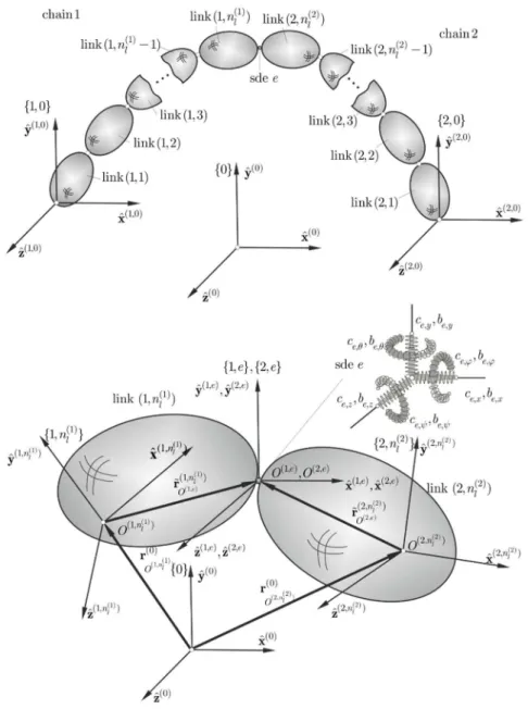
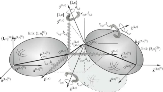
2 GENERAL MODEL OF THE SPRING-DAMPING ELEMENT
Figure 2: Links (1,n(1)l ) and (2,nl(2)) connected by means of the spring-damping element.
(1) (1) (1)
(1, ) (1, ) (1, )
ˆ ˆ ˆ
{x nl ,y nl ,y nl } – coordinate system connected with link (1, (1))
l
n
(2) (2) (2)
(2, ) (2, ) (2, )
ˆ ˆ ˆ
{x nl ,y nl ,y nl } – coordinate system connected with link (2, (2))
l
n
(1, ) (1, ) (1, )
ˆ ˆ ˆ
{x e,y e,y e}, {xˆ(2, )e,ˆy(2, )e,ˆy(2, )e} – coordinate system of sdee connected with link(1,nl(1)) and (2,nl(2)), respectively
, , , { , , , , , }
e e x y z c ab
a aÎ j q y – spring and damping coefficients of sdee, respectively
It is assumed that the axes of the coordinate system coincide with the principal elastic axes of
(moment) directed along the specified axis, displacement (rotation) is only in the direction (around) this axis.
The homogeneous transformation matrices from the local coordinate systems (1)
{1,nl } and (2)
{2,nl } to the initial coordinate system {0} can be written in the forms
(1) (1)
(1) (1, ) (1, ) (0) (1, )
, 1
l
l nl
n n
O
é ù
ê ú
ê ú
=ê ú
ê ú
ë û
R r
T
0 (1.1)
(2) (2)
(2) (2, ) (2, ) (0) (2, )
, 1
l
l nl
n n
O
é ù
ê ú
ê ú
=ê ú
ê ú
ë û
R r
T
0 (1.2)
where (1) (2)
(1, ) (2, ) (0) , (0)
nl nl
O O
r r – vectors describing the origins of the coordinate systems (1)
{1,nl } and (2)
{2,nl } in {0}, respectively (1) (2)
(1, ) (2, )
,
l l
n n
R R – rotary matrices describing the direction cosines of the axes of the
coordi-nate systems (1)
{1,nl }in {0}and {2,nl(2)}in {0}, respectively.
It is assumed that the position and orientation of systems {1, }e and {2, }e in {1,nl(1)} and (2)
{2,nl } are described by matrices with constant elements.
(1) (1, ) (1, ) (1, )
(1, )
, 1
l e
n e e
O
é ù
ê ú
= ê ú
ê ú
ë û
R r
T
0
(2.1)
(2) (1, ) (2, ) (2, )
(2, )
, 1
l e
n e e
O
é ù
ê ú
= ê ú
ê ú
ë û
R r
T
0
(2.2)
where (1, )(1) (2, )(2) (1, ) (2, )
,
l l
e e
n n
O O
r r
– vectors describing the origin of coordinate systems {1, }e and {2, }e in
(1)
{1,nl } and {2, (2)}
l
n , respectively,
(1, ) (2, )
,
e e
R
R
– rotary matrices describing the orientation of coordinate systems {1, }e and{2, }e in {1,nl(1)}, and (2)
{2,nl }, respectively.
If sde e is undeformed, then the coordinate systems {1, }e and {2, }e coincide with each other.
It is assumed that the principal elastic axes of sdee coincide with the axes of system {1, }e
connected with link {1, (1)}
l
n . This means that the translational and rotational deformations of sde
e will be described in the coordinate system {1, }e . The considered situation is presented in Fig. 3.
Figure 3: The sde connecting with link {1,nl(1)}.
According to Eqs. (1) and (2), the homogeneous transformation matrices from systems {1, }e
and {2, }e to system {0}have the following forms
(1) (1)
(1)
(1) (1, ) (1, ) (1, )
(1, ) (0) (1, ) (1, ) (1, ) (0) (1, )
(1, ) (1, ) ,
1 1
1
l l
e e
l nl
n e n e
n
e e O
O O
é ù é ù é ù
ê ú ê ú ê ú
ê ú
= =ê ú êê úú= ê ú
ê ú
ê úë û ë û
ë û
R r R r R r
T T T
0 0
0
(3.1)
(2) (1)
(2)
(2) (2, ) (2, ) (2, )
(2, ) (0) (2, ) (2, ) (2, ) (0) (2, )
(2, ) (2, ) ,
1 1
1
l l
e e
l nl
n e n e
n
e e O
O O
é ù é ù é ù
ê ú ê ú ê ú
ê ú
= =ê ú êê úú= ê ú
ê ú
ê úë û ë û
ë û
R r R r R r
T T T
0 0
0
(3.2)
where R(1, )e =R(1,nl(2))R(1, )e ,
(2) (2, ) (2, )e = nl (2, )e
R R R ,
(1) (1)
(1, ) (1, ) (1,(1)) (1, ) (1, )
(0) l l (0)
e e
nl
n n
O O
O
= +
r R r r ,
(2) (2)
(2, ) (2, ) (2,(2)) (2, ) (2, )
(0) l l (0)
e e
nl
n n
O O
O
= +
r R r r
Let us assume that the translational and rotational displacements, being deformations of sde e,
have the components
, , , ,
T tr
e de x de y de z
é ù
= êë úû
, , , .
T rot
e = êéëdej deq deyùúû
d (4.2)
The potential energy of spring deformation and the Rayleigh dissipation function (translational and rotational) of sde e can be presented as follows
( )
, 1 , 2 T tr tr tr tr p e e e eE = d C d (5.1)
( )
, 1 , 2 Trot rot rot rot p e e e e
E = d C d (5.2)
( )
1
, 2
T tr tr tr tr e e e e
R = d B d (5.3)
( )
1
, 2
T
rot rot rot rot e e e e
R = d B d (5.4)
where , , , 0 0 0 0 0 0 e x tr
e e y
e z c c c é ù ê ú ê ú
= ê ú
ê ú ê ú ê ú ë û C , , , , 0 0 0 0 0 0 e rot e e e c c c j q y é ù ê ú ê ú
= ê ú
ê ú ê ú ê ú ë û C , , , , 0 0 0 0 0 0 e x tr
e e y
e z b b b é ù ê ú ê ú
= ê ú
ê ú ê ú ê ú ë û B , , , , 0 0 0 0 0 0 e rot e e e b b b j q y é ù ê ú ê ú
= ê ú
ê ú
ê ú
ê ú
ë û
B .
The coordinates of the origin of system {2, }e can be expressed in the coordinates of system
{1, }e by the formula
(2, ) (2, ) (1, ) (2, ) (1, )
(1, ) (0) (0) (2, ) (2, ) (1, ) (1, )
e e e e e
e e e e e
O = O - O = O - O
r r r T r T r (6)
and vector dtre as
(
)
(2, ) (2, ) (1, )
(1, ) (2, ) (2, ) (1, ) (1, )
,
e e e
e e e
tr e e
e = O = O - O
d Jr J T r T r (7)
where 1 2 3
1 0 0 0 0 1 0 0 0 0 1 0
é ù
ê ú
ê ú é ù
=ê ú=êë úû
ê ú
ê ú
ë û
J j j j 0 .
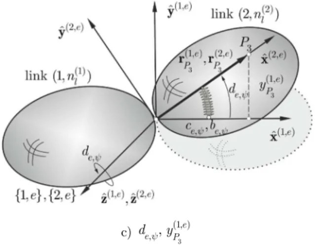
In order to calculate the components of vector drote , it is assumed that the rotational angles
,
,
,,
,e e e
1 1
(1, ) , (2, ),
e P
e e
P z d
y
j = (8.1)
2 2
(1, ) , (2, ),
e P
e e
P x d
z
q = (8.2)
3 3
(1, ) , (2, ),
e P
e e
P y d
x
y = (8.3)
where
1
(1, )e P
z – coordinate of point P1 in {1, }e ,
1 1
(2, ) (2, )
0 0 1
T
e e
P yP
é ù
= êë úû
r ,
2
(1, )e P
x – coordinate of point P2 in {1, }e ,
2 2
(2, ) (2, )
0 0 1
T
e e
P zP
é ù
= êë úû
r ,
3
(1, )e P
y – coordinate of point P3 in {1, }e ,
3 3 (2, ) (2, )
0 0 1
T e e
P xP
é ù
= êë úû
r .
a)
1
(1, ) , ,
e e P d j z
b)
2
(1, ) ,,
c)
3
(1, ) , ,
e e P d y y
Figure 4: Displacements and rotational angles insdee.
Displacements
1 2 3
(1, ) (1, ) (1, )
, ,
e e e
P P P
z x y can be solved from the formulas
( )
( )
1 1 1
1 1
(1, ) (1, ) (2, ) (2, ) (2, ) (1, ) (2, ) 2 3
0 0 1 0 0 ,
1
e e e e e T e e
P P P
z - y
-é ù
é ù ê ú
é ù
=êë úû = ê ú ê ú
ë û ê ú
ë û
j
T T r j T T (9.1)
( )
( )
2 2 2
1 1
(1, ) (1, ) (2, ) (2, ) (2, ) (1, ) (2, ) 3 1
1 0 0 0 0 ,
1
e e e e e T e e
P P P
x - z
-é ù
é ù ê ú
é ù
=êë úû = ê ú ê ú
ë û ê ú
ë û
j
T T r j T T (9.2)
( )
( )
3 3 3
1 1
(1, ) (1, ) (2, ) (2, ) (2, ) (1, ) (2, ) 1 2
0 1 0 0 0 .
1
e e e e e T e e
P P P
y - x
-é ù
é ù ê ú
é ù
=êë úû = ê ú ê ú
ë û ê ú
ë û
j
T T r j T T (9.3)
Having Eqs. (3) and (8), we obtain
( ) ( )
( )
( ) (
)
(2, ) (1, )
1 1
(2, ) (1, ) 1
(2, ) (0) (1, ) (1, ) (0)
(1, ) (2, ) 2
3
(2, ) (1, ) (2, ) (1, ) (0) (0)
3 2 3
( )* 0
1 1 1
e e
e e
T T e
e e
e e T O
O
P P
T T
e T e e T e
P O O
z y
y
é ù é ù é ù
ê - úê ú
é ùê ú ê ú
= êë úûê úê úê ú=
ê ú ê úë û
ê ú ë û
ë û
æ ö÷
ç ÷
çç ç
= çç +
-çççè ø
j
R r
R R r
j
0 0
j R R j j R r r
÷÷÷÷÷÷÷÷.
(10)
If we assume that the origins of systems {1, }e and {2, }e coincide with each other, then we take
into account that formula (*) in Eq. (10) is equal to zero and can be written as follows
( )
1 1
(1, ) (2, ) (1, ) (2, )
3 2
T e e T e e P P
z =y j R R j . (11.1)
( )
2 2
(1, ) (2, ) (1, ) (2, )
1 3
T e e T e e P P
x =z j R R j (11.2)
and
( )
3 3
(1, ) (2, ) (1, ) (2, )
2 1
T e e T e e P P
y =x j R R j . (11.3)
The components of vectors derot can be calculated from Eq. (8) as follows
( )
(1, ) (2, ), 3 2
T e e T
e
d j = j R R j , (12.1)
( )
(1, ) (2, ), 1 3
T e e T
e
d q = j R R j , (12.2)
( )
(1, ) (2, ), 2 1
T e e T
e
d y = j R R j . (12.3)
After taking into account Eqs. (7) and (12), the potential energy of spring deformation and the Rayleigh dissipation function of sde e can be written in the following way
, , ,
1 2
tr rot T p e p e p e e e e
E =E +E = d C d , (13.1)
1 2
tr rot T e e e e e e
R =R +R = d B d , (13.2)
where tr e e rot e é ù ê ú
= ê ú
ê ú ë û d d d , tr e e rot e é ù ê ú
= ê ú
ê ú
ë û
C 0
C
0 C ,
tr e e rot e é ù ê ú
= ê ú
ê ú
ë û
B 0
B
0 B ,
(
)
(
)
(
)
( )
( )
( )
(2, ) (1, ) (2, ) (1, ) (2, ) (1, )
(2, ) (1, ) (2, ) (1, ) 1
(2, ) (1, ) (2, ) (1, ) 2
(2, ) (1, ) (2, ) (1, ) 3
(1, ) (2, )
3 2
(1, ) (2, )
1 3
(1, ) (2, 2 0 0 0 e e e e e e e e
T e e
O O
e e
T e e
O O
e e
T e e
O O T e e T e T e e T T e T
é ù
-ê ú
ë û
é ù
-ê ú
ë û
é ù
-ê ú
ë û
=
j T r T r
j T r T r
j T r T r
d
j R R j
j R R j
j R R
) 1 e é ù ê ú ê ú ê ú ê ú ê ú ê ú ê ú ê ú ê ú ê ú ê ú ê ú ê ú ê ú ê ú ê ú ê ú
ë j û
,
(
)
(
)
(
)
( )
( )
(2, ) (1, ) (2, ) (1, ) (2, ) (1, )
(2, ) (1, ) (2, ) (1, ) 1
(2, ) (1, ) (2, ) (1, ) 2
(2, ) (1, ) (2, ) (1, ) 3
(1, ) (2, ) (1, ) (2, )
3 2 3 2
1 0 0 0 e e e e e e e e
T e e
O O
e e
T e e
O O
e e
T e e
O O
T T
e e e e
T T
e
T
é ù
-ê ú
ë û
é ù
-ê ú
ë û
é ù
-ê ú
ë û
=
+
j T r T r
j T r T r
j T r T r
d
j R R j j R R j
j
( )
( )
( )
( )
(1, ) (2, ) (1, ) (2, )
3 1 3
(1, ) (2, ) (1, ) (2, )
2 1 2 1
T T
e e T e e
T T
e e e e
T T é ù ê ú ê ú ê ú ê ú ê ú ê ú ê ú ê ú ê ú ê ú ê ú
ê + ú
ê ú
ê ú
ê ú
ê + ú
ê ú
ë û
R R j j R R j
j R R j j R R j
( ) ( ) ( ) ( ) ( ) ( , ) ( , ) ( , ) ( , ) ( , ) ( , )
1,2 1 1 ,
c c
dof c dof c
l l
c l
n c e n
c n c n
c e c e
k k k
c n c k k k q q q = = = ¶ = = 
å
Tå
T T
( ) ( ) ( ) ( ) ( ) ( , ) ( , ) ( , ) ( , ) ( , ) ( , )
1,2 1 1 .
c c
dof c dof c
l l
c l
n c e n
c n c n
c e c e
k k k
c n c k k k q q q = = = ¶ = = 
å
Rå
R R
In order to use these formulas, the derivatives of Eq. (13) for the generalized coordinates
de-scribing the motion of links (1)
{1,nl } and {2,nl(2)} in the initial coordinate system {0}can be calcu-lated as follows
( ) ( ) ( ) , ( , ) ( , ) 1,2 1, , c c l l c l T
p e e
e e
c n c n
c
k k
k n
E
q = q
= ¶ ¶ = ¶ ¶ d C d
, (14.1)
( ) ( ) ( ) ( , ) ( , ) 1,2 1, , c c l l c l T e e e e
c n c n
c
k k
k n
R
q = q
= ¶ ¶ = ¶ ¶ d B d
, (14.2)
where
( )
( )
( )
(1, ) (1, ) (1, ) (1) (1, ) (1, ) 1 (1, ) (1, ) 2 (1, ) (1, ) 3 (2, ) (1, ) (1, ) 3 2 (2, ) (1, ) 1 3 (2, ) (1, ) 2 1 0 0 0 e e e l e T e k O e T e k O e T e k O e T e T e n k k T e T e k T e T e k qé-é ù ù
ê êë úû ú
ê é ù ú
ê- ê ú ú
ê ë û ú
ê é ù ú
ê- ê ú ú
ê ë û ú
¶ ê ú
= ê ú
¶ ê ú
ê ú ê ú ê ú ê ú ê êë û
j T r
j T r
j T r
d
j R R j
j R R j
j R R j
ú ú ,
( )
( )
( )
(2, ) (2, ) (2, ) (2) (2, ) (2, ) 1 (2, ) (2, ) 2 (2, ) (2, ) 3(1, ) (2, ) (2, )
3 2
(1, ) (2, )
1 3
(1, ) (2, )
2 1 0 0 0 e e e l e T e k O e T e k O e T e k O e T e T e n k k T e T e k T e T e k q
éé ù ù
êêë úû ú
êé ù ú
êê ú ú
êë û ú
êé ù ú
êê ú ú
êë û ú
¶ ê ú
= ê ú
ê ú
¶ ê ú
ê ú ê ú ê ú ê ú ê ú êë û
j T r
j T r
j T r
d
j R R j
j R R j
j R R j
ú ,
( )
( )
( )
(1, ) (1, ) (1, ) (2) (1, ) (1, ) 1 (1, ) (1, ) 2 (1, ) (1, ) 3 (2, ) (1, ) (1, ) 3 2 (2, ) (1, ) 1 3 (2, ) (1, ) 2 1 0 0 0 e e e l e T e k O e T e k O e T e k O e T e T e n k k T e T e k T e T e k qé-é ù ù
ê êë úû ú
ê é ù ú
ê- ê ú ú
ê ë û ú
ê é ù ú
ê- ê ú ú
ê ë û ú
¶ ê ú
= ê ú
¶ ê ú
ê ú ê ú ê ê ê êë û
j T r
j T r
j T r
d
j R R j
j R R j
j R R j
ú ú ú ú ,
( )
( )
( )
(2, ) (2, ) (2, ) (2) (2, ) (2, ) 1 (2, ) (2, ) 2 (2, ) (2, ) 3(1, ) (2, ) (2, )
3 2
(1, ) (2, )
1 3
(1, ) (2, )
2 1 0 0 0 e e e l e T e k O e T e k O e T e k O e T e T e n k k T e T e k T e T e k q
éé ù ù
êêë úû ú
êé ù ú
êê ú ú
êë û ú
êé ù ú
êê ú ú
êë û ú
¶ ê ú
= ê ú
ê ú
¶ ê ú
ê ú
ê ú
ê ú
ê
êêë û
j T r
j T r
j T r
d
j R R j
j R R j
j R R j
The formulas presented here can be used to model any joints. Clearances are neglected in these formulas.
The model presented here will be used to derive equations of motion of the one-DOF RSRRP linkage mechanism.
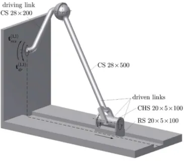
3 DYNAMICS ANALYSIS OF THE SPATIAL LINKAGE MECHANISM
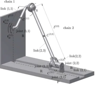
An example of using the replacement models of the spherical and prismatic joint in the one-DOF RSRRP linkage mechanism is shown below (Haug, 1989). The mechanism consists of four rigid links connected to a fixed base – Fig. 5.
Figure 5: Analyzed spatial mechanism.
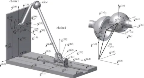
The mechanism considered here was divided in the place of spherical joint S for a replacement model of a spherical joint and the cut-joint technique (Fig. 6a). Two open-loop kinematic chains joined with the fixed base were obtained: 1 – is formed by link (1,1), and 2 is formed by links (2,1), (2, 2), (2, 3). For a replacement model of a revolute joint, the mechanism is cut in the place of revolute joint R (Fig. 6b). This approach also allows to obtain a system with two open-loop kin-ematic chains but built with: 1 – is formed by links (1,1), (1,2), and 2 is formed by links (2,1),
(2, 2). In both cases link (1,1) is the driving link loaded by torque t(1,1)dr and resistance torque t(1,1)res . The local coordinate systems were attached to the particular links according to the
Denavit-Hartenberg notation (Denavit and Denavit-Hartenberg, 1955). The fixed coordinate system {1, 0}, related to
refer-ence system {1, 0}(Figs. 7a and b). In the cut-joint technique, joint forces fS x, , fS y, , fS z, and ,
S x
-f , -fS y, , -fS z, , acting on chains 1and 2, respectively, in accordance with the versor directions of the global reference system {1, 0} (Fig. 7c), are applied in the place of the mechanism cut.
a) replacement model of the spherical joint, cut-joint technique
b) replacement model of the revolute joint
a) replacement model of the spherical joint
b) replacement model of the revolute joint
c) cut-joint technique
The motion of chain c is described by the joint coordinate vectors:
( ) ( )
( ) ( , ) ( , )
1,2 1,...,
c c
l l
c dof
c n c n
j
c j n
q
= =
æ ö÷
ç =ççè ÷÷ø
q , (15)
where:
1) for chain :
– replacement model of the spherical joint, cut-joint technique
( )
= é ù= = ê ú
ë û
(1,1) (1,1) (1,1) 1
j j
q y
q ,
– replacement model of the revolute joint
( )
(1,2) (1,2) (1,1) (1,2) (1,2) (1,2)
1,...,4
T j j
q y y q j
=
é ù
= = ê ú
ë û
q ,
2) for chain :
– replacement model of the spherical joint and cut-joint technique
( )
(2,3) (2,3) (2,1) (2,2) (2,3) 1,2,3
T j
j
q d y y
=
é ù
= = ê ú
ë û
q ,
– replacement model of the revolute joint
( )
(2,2) (2,2) (2,1) (2,2) 1,2
T j
j
q d y
=
é ù
= = êë úû
q .
The homogeneous transformation matrices from the local systems attached to the links to the global reference system {1, 0} are determined according to the relationship:
( )
( , ) ( , 1) ( , ) 1,2
1, , c l
c p c p c p
c
p n
-=
=
=
T T T
,
(16)
where T( ,0)c = I, 1) for chain :
– replacement model of the spherical joint, cut-joint technique
é - ù
ê ú
ê ú
é ù ê ú
ê ú
=ê ú= ê ú
ê ú
ê ú
ë û ê ú
ê ú
ê ú
ë û
(1,1)
(1,1) (1,1) (1,0)
(1,1) (1,1) (1,1) (1,1)
c s 0 0
s c 0 0
1 0 0 1 0
0 0 0 1
O
y y
y y
R r
T
0 ,
é - ù
ê ú
ê ú
é ù ê ú
ê ú
=ê ú= êê úú
ê ú
ë û ê ú
ê ú ê ú ë û (1,1) (1,1) (1,1) (1,0)
(1,1) (1,1) (1,1) (1,1)
c s 0 0
s c 0 0
1 0 0 1 0
0 0 0 1
O y y y y R r T 0 , (1,2)
(1,2) (1,2) (1,2) (1,2) (1,2) (1,2) (1,2) (1,2) (1,2) (1,2) (1,2) (1,2)
(1,1)
(1,2) (1,2) (1,2) (1,2) (1,2) (1,2) (1,2) (1,2) (1,2) (1,2) (1,2) (1,2)
c c c s s s c c s c s s 0
s c s s s c c s s c
1 O
y q y q j y j y q j y j
y q y q j y j y q j
- +
é ù +
-ê ú
=ê ú=
ê ú ë û R r T 0
(1,2) (1,2) (1,1)
(1,2) (1,2) (1,2) (1,2) (1,2)
c s
-s c s c c 0
0 0 0 1
l
y j
y q j q j
é ù ê ú ê ú ê ú ê ú ê ú ê ú ê ú ê ú ë û ,
2) for chain :
– replacement model of the spherical joint, cut-joint technique
(2,0) (2,1) (2,0)
(1,0) (2,0) (1,0)
(2,0) (2,1) (2,1)
(2,1)
0 1 0 0 1 0 0 0
0 1 0 0
1 0 0
0 0 1
1 1 0 0 1 0
0 0 0 1
0 0 0 1
O O yO
d
é - ù é ù
ê ú ê ú
ê ú ê ú
é ù é ù ê
-ú ê ú
ê ú ê ú
=ê ú ê ú= êê ú ê ú
ú ê ú
ê ú ê ú
ë û ë û ê ú ê ú
ê ú êë úû
ë û
R r R r
T
0 0
,
é - ù
ê ú
ê ú
é ù ê ú
ê ú
=ê ú= ê ú
ê ú
ê ú
ë û ê ú
ê ú ê ú ë û (2,2) (2,2) (2,1) (2,2) (2,2) (2,1)
(2,2) (2,2) (2,2) (2,2)
c s 0
s c 0 0
1 0 0 1 0
0 0 0 1
O O x y y y y R r T 0 ,
é - ù
ê ú
ê ú
é ù ê ú
ê ú
=ê ú= êê- - úú
ê ú
ë û ê ú
ê ú ê ú ë û (2,3) (2,3) (2,3) (2,2) (2,3) (2,3) (2,3) (2,3)
c s 0 0
0 0 1 0
1 s c 0 0
0 0 0 1
O y y y y R r T 0 ,
– replacement model of the revolute joint
(2,0) (2,1) (2,0)
(1,0) (2,0) (1,0)
(2,0) (2,1) (2,1)
(2,1)
0 1 0 0 1 0 0 0
0 1 0 0
1 0 0
0 0 1
1 1 0 0 1 0
0 0 0 1
0 0 0 1
O O yO
d
é - ù é ù
ê ú ê ú
ê ú ê ú
é ù é ù ê
-ú ê ú
ê ú ê ú
=ê ú ê ú= êê ú ê ú
ú ê ú
ê ú ê ú
ë û ë û êê ú ê ú
ú êë úû
ë û
R r R r
T
0 0
é - ù
ê ú
ê ú
é ù ê ú
ê ú
=ê ú= ê ú
ê ú
ê ú
ë û ê ú
ê ú ê ú ë û (2,2) (2,2) (2,1) (2,2) (2,2) (2,1)
(2,2) (2,2) (2,2) (2,2)
c s 0
s c 0 0
1 0 0 1 0
0 0 0 1
O O x y y y y R r T 0 , ( , ) ( , ) ( , ) ( , )
s
a
b g=
sin
a
b g, c
a
b g=
cos
a
b g.
The homogeneous transformation matrices from the local systems sde e to the global reference
system {1, 0} are determined according to the relationship:
( ) ( , ) ( , ) ( , ) 1,2 c l c n
c e c e
c= =
T T T , (17)
where:
– replacement model of the spherical joint
(1, )
(1,1)
(1, ) (1,1)
(1, )
1 0 0 0
0 1 0
0 0 1 0
1
0 0 0 1
e
e
e O l
é ù
ê ú
ê ú
é ù ê ú
ê ú
=ê ú= ê ú
ê ú
ê ú
ë û ê ú
ê ú ë û R r T 0 , (2, )
(2, ) (2, ) (2,3)
(2, ) (2, ) (2, ) (2,3)
(2, ) (2, ) o
0 c s 0
0 s c
, 60 ,
1 1 0 0 0
0 0 0 1
e
e e
e e e
e O l e
b b
b b b
é ù
ê ú
ê ú
é ù ê - ú
ê ú
=ê ú=êê úú =
ê ú
ë û ê ú
ê ú ê ú ë û R r T 0
– replacement model of the revolute joint
(1, )
(1, ) (1, ) (1,2) (1,2)
(1, ) (1, ) (1, )
(1, ) (1, ) o
0 -s c
0 c s 0
, 60
1 1 0 0 0
0 0 0 1
e
e e
e e e
e O e
l
b b
b b b
é ù
ê ú
ê ú
é ù ê ú
ê ú
=ê ú=ê ú =
ê- ú
ê ú
ë û ê ú
ê ú ê ú ë û R r T 0 , (2, ) (2,2) (2, ) (2, )
0 1 0 0
1 0 0 0 .
0 0 1 0
1
0 0 0 1
e
e
e O
é ù
ê ú
é ù ê- ú
ê ú ê ú
=ê ú=ê ú
ê ú ê ú
ë û ê ú
4 SYNTHESIS OF THE EQUATIONS OF MOTION AND THE ALGORITHM FOR THEIR
SOLU-TION
The equations of motion of chains are determined by using the formalism of Lagrange equations on
the basis of algorithms given in a monograph by Jurevič ed. , 1984. The structure of these
equa-tions is different depending on the proposed analysis method: 1. Replacement model of the spherical joint
,
(1,1) (1,1) (1,1) (1,1) (1,1) (1,1) (1,1) (2,3) (2,3) , (2,3) (2,3) (2,3) tr tr p e e
dr res tr tr
p e e
E R
E R
é æç¶ ¶ ö÷ ù
ê ç ÷÷ ú
- + +
-ê çç ÷÷ ú
é ù é ù ê ççè¶ ¶ ÷÷ø ú
ê ú ê ú=ê ú
ê ú ê ú ê æ ö ú
ê ú ê ú ê ç¶ ¶ ÷÷ ú
ë û ë û ê -çç + ÷÷ ú
ç
ê çç¶ ¶ ÷÷÷ ú
ê è ø ú
ë û
e t t
q q
A 0 q
0 A q
e q q
, (18.1)
2. Replacement model of the revolute
,
(1,2) (1,1) (1,1) (1,2) (1,2) (1,2) (1,2) (2,2) (2,2) , (2,2) (2,2) (2,2) p e e
dr res
p e e
E R
E R
é æç¶ ¶ ö÷ ù
ê ç ÷÷ ú
- + +
-ê çç ÷÷ ú
é ù é ù ê ççè¶ ¶ ÷÷ø ú
ê ú ê ú=ê ú
ê ú ê ú ê æ ö ú
ê ú ê ú ê ç¶ ¶ ÷÷ ú
ë û ë û ê -çç + ÷÷ ú
ç
ê çç¶ ¶ ÷÷÷ ú
ê è ø ú
ë û
e t t
q q
A 0 q
0 A q
e q q
, (18.2)
3. Cut-joint technique
(1,1) (1,1) (1,1) (1,1) (1,1) (1,1) (2,3) (2,3) (2,3) (2,3)
(1,2) (1,1)T (2,3)T
dr res
S
é - ù é ù é + - ù
ê ú ê ú ê ú
ê ú ê ú ê ú
ê úê ú=ê ú
ê ú ê ú ê ú
ê - ú ê ú ê ú
ê ú êë úû êë úû
ë û
A 0 D q e t t
0 A D q e
f c
D D 0
, (18.3)
where { } ( ) ( ) ( ) ( ) ( )
( , 1) ( , 1) ( , ) ( , )
( , ) ( , ) ,
, 1, ,
( , ) ( , ) ( , ) ( , )
, , , , 1, , , 1,...,
max , 1,...,
( , ) , , , t c c l l c l c l c l
c i c j c i
dof dof dofc j dof
c n c n
i j
i j n
n
c n c l c p c p
i j i j i j n k n l k n
i j p
l i j
l n c p i j a a - -= + + = = = = æ ö÷ ç
=ççè ÷÷ø
æ ö÷
ç
= =ççè ÷÷÷ø
=
å
A A
A A A
{
}
( ) ( )
( ) ( )
( )
( , 1)
( , ) ( ( , ) ( , ) 1, , ( , ) ( , ) ( , ) ( , ) ( , )
1, , 1,...,
( , ) ( , ) ( , ) ( , ) , , 1 , , tr c c l l c l c l c l c i c i dof dof c dof T
c n c n i
i n n
c n c p c p
i i i
p i
c p c p
i n k
i p k n
n
c p c p c p c p
i i m n
m n h h -= = + = = = æ ö÷ ç =ççè ÷÷ø
é ù
= - ê + ú
ë û
æ ö÷
ç
=ççè ÷÷÷ø
=
å
e e
e h g
h
T H T
, )
( , 1)
( , )
( , )
( , ) ( , )
( , ) ( , )
1, , 1,..., ( ) ( , ) ( , ) ( , ) 2 , 0 , p c i c i dof dof c p
c p c p m n c p
c p
i n k
i p k n
c c p c p T c p
i i C
q q
g
g m g
- +
= =
æ ö÷
ç
=ççè ÷÷÷ø
é ù
= ê ú
ë û
å
g
j T r
(1,1) (1,1) (1,1)
replacement model of the spherical joint, cut-joint technique,
replacement model of the revolute joint,
dr T dr dr t t ìé ù ï -ïê ú ïë û ï
= íïéï ù
-ê ú ïë û ïî t 0 (1,1) (1,1) (1,1)
replacement model of the spherical joint, cut-joint technique,
replacement model of the revolute joint,
res T res res t t ìé ù ï -ïê ú ïë û ï
= íïéï ù
-ê ú ïë û ïî t 0 ( ) ( ) ( ) ( ) ( ) ( ) ( , ) ( , ) ( , ) ( , ) ( , ) 1 c
c T c c c
l
l l l l
c l
c n c n c n c n c n
S n S
é ù
= ê ú
ê ú
ë û
D J T r T r
(2) (1)
(1,2) (2,3) (2,3) (2,3) (2,3) (1,1) (1,1) (1,1) (1,1)
, ,
, 1 , 1
l l
n n
i j i j S i j i j S
i j i j
q q q q
= =
éæç ö÷ æç ö÷ ù
êç ÷÷ ç ÷÷ ú
= êçç ÷÷ -çç ÷÷ ú
êççè ÷÷ø ççè ÷÷ø ú
ê ú
ë û
å
å
c J T r T r .
The structure and number of equations were different for each of the methods, thus different al-gorithms were used to solve them.
For the replacement models of a spherical and revolute joint, a system of four and six ODEs of second order was obtained, respectively (Figs. 8a and b). At the beginning of the procedures as-sumed here the configuration of the mechanism was determined in conditions of static equilibrium of its links. Minimal movements of the links, caused by gravity forces, result from the flexibility of the replacement model. By performing this part of the procedures (i.e. statics analysis), a system of non-linear algebraic equations, obtained on the basis of the differential equation, is solved by the Newton-Raphson method. The positions of the links determined in such a way also determine the initial conditions in the dynamics analysis of the mechanism.
Addition-al cAddition-alculations using the recursive Newton-Euler Addition-algorithm were performed in order to determine the joint forces and torques in the other joint.
In both cases the components of the acceleration vectors are broken down into a system of ODEs of first order and solved by the Runge-Kutta method of the fourth order with a constant integra-tion step.
a) replacement model of the spherical joint
c) cut-joint technique
Figure 8: Algorithms of solving equations of statics and dynamics of the mechanism in question.
5 NUMERICAL CALCULATION RESULTS
The parameters and initial configuration of the mechanism are presented in Fig. 9. It was assumed that at the initial moment of the mechanism’s motion the symmetry axes of all its links are in the vertical plane ˆy(1,0) ˆz(1,0 ) of the global reference system {1, 0}.
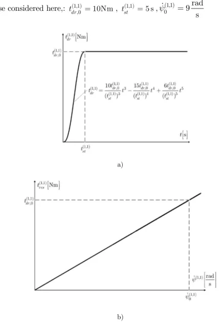
The assumed time courses of the value of the driving torque tdr(1,1) and the resistance torque (1,1)
res
t are presented in Figs. 10a and b, respectively. The following parameters were taken into
ac-count in the case considered here,: (1,1)
,0 10Nm dr
t = , tst(1,1)=5 s, (1,1)0 9rad s
y =
a)
b)
Figure 10: Time course of: a) driving torque, b) resistance torque.
It is assumed that the analysis time is 15s. A constant integration step equal to
10 s
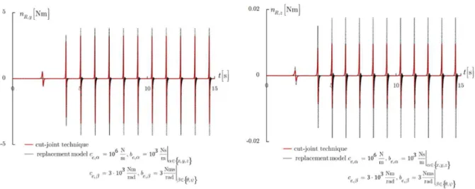
-4 is as-sumed.A comparison of the numerical results of the courses of components of joints forces fS , fR and
Figure 11: Courses of components of joint forces fS, fR and torque nR.
As can be observed, sufficient compliance results are obtained even at relatively low values of stiffness and damping coefficients and a large value of the integration step size.
Numerical tests carried out with different integration steps did not confirm the necessity of us-ing a stabilization method of constraint equations. The Euclidean norm determined for the integra-tion step equal to
10 s
-4 has an insignificant value (less than10 m
-6 ).6 CONCLUSIONS
The general model of a flexible connection of links is presented in the paper. The connection is done by means of spring-damping elements. It was derived the formulas for the energy of the spring de-formation, the Rayleigh dissipation function and their derivatives convenient to introduce them in Lagrange's equations of the second order. The formalism of homogeneous transformations was used to derive these formulas. The general model presented here can be used to formulate the replace-ment model of any joint.
The models of the spherical and revolute joint are presented as an example of the general mod-el. The results for the replacement models were compared by using the cut-joint technique. Good compatibility can be observed of the results obtained here.
In the author’s opinion, the use of replacement models can be efficient when the flexibility and clearances are taken into account.
References
Adamiec-Wójcik I., Maczyński A., Wojciech S., (2008) Application of homogeneous transformations in modeling of the offshore systems, The Transport and Communication Press, Warsaw (in Polish)
Augustynek K., (2010) Dynamics analysis of the spatial mechanisms with flexible links, PhD thesis, Radom Universi-ty, Radom (in Polish)
Blajer, W., (1998) The methods for dynamics of the multibody systems, Radom University Press, Radom (in Polish) Craig J.J., (1989) Introduction to robotics. Mechanics and control, Addison-Wesley Publishing Company, Inc. Denavit J., Hartenberg R.S., (1955) A kinematic notation for lower-pair mechanisms based on matrices, ASME Journal of Applied Mechanics, June
Farid M., Lukasiewicz S. A., (2000) Dynamic modeling of spatial manipulators with flexible links and joints, Com-puters and Structures 75, 419-437
Frączek J., (2002) Modeling of the spatial mechanisms using the methods for multibody system, Warsaw University of Technology Press, No. 196, Warsaw (in Polish)
Ganiev R.F., Kononenko V.O., (1976) Vibration of rigid bodies, Nauka, Moscow (in Russian)
Hanzaki R. A., Saha K. S.,·Rao P.V.M., (2009), An improved dynamic modeling of a multibody system with spheri-cal joints, Multibody System Dynamics, 21, 325–345
Harris C.M., Piersol A.G., (2010) Harries’ shock and vibration handbook, 6th edition, McGraw Hill
Haug E.J., (1989) Computer aided kinematics and dynamics of mechanical systems, Vol. 1: Basic methods, Allyn and Bacon
Jurevič E.I., (1984) Dynamics of robots, Nauka, Moscow (in Russian)
Nergut D., Ottarsson G., Rampalli R., Sajdak A., (2006) On an implementation of the Hilber-Hughes-Taylor method in the context of index 3 differential-algebraic equations of multibody dynamics, DET2005-85096
Schiehlen W., Rükgauer A., Schirle Th., (2000) Force Coupling versus differential algebraic description of con-strained multibody systems, Multibody System Dynamics, 4, 317-340
Szczotka M., (2004) Modeling of the motion of the vehicles with taking into account different transmission systems, PhD thesis, Bielsko-Biala, (in Polish)
Urbaś A., (2011) Dynamic analysis and control of the working machines with flexibly supported base, PhD thesis, Bielsko-Biala (in Polish)
Urbaś A., Szczotka M., Wojciech S., (2011) The influence of flexibility of the support on dynamic behavior of a crane, International Journal of Bifurcation and Chaos, 21(10), 2963-2974
Wang J., Gosselin C.M., Cheng L., (2002) Modeling and simulation of robotic systems with closed kinematic chains using the virtual spring approach, Multibody System Dynamics, 7, 145-170