Eigenvalue based inverse model of beam for structural
modifi-cation and diagnostics. Part II: Examples of using
Abstract
In the work, in order to solve the inverse problem, i.e. the problem of finding values of the additional quantities (mass, elasticity), the beam inverse model was proposed. Analysis of this model allows finding such a value of additional mass (elasticity) as a function of its localization so that the free vi-bration frequency changes to desirable value. The criteria for choice of the “proper” pair (mass – its position), including the criterion allowing changing the position of the vibration node of the second mode of the free vibrations, were given. Analysis of the influence of uncertainties in the determina-tion of the addidetermina-tional quantity value and its posidetermina-tion on the desired free vibration frequency was carried out, too. The proposed beam inverse model can be employing to iden-tification of the beam cracks. In such a case, the input quan-tity is free vibration frequency measured on the damaged object. Each determined free-vibration frequency allows de-termining the flexibility curve for the spring modeling crack as a function of its position. The searched parameters of the crack (its depth and position) are indicated by the com-mon point of two arbitrary curves. Accuracy of crack pa-rameters determination depends on accuracy (uncertainty) of frequency measurement. Only some regions containing the searched crack parameters can be obtained in such a situation.
Keywords
inverse model, structural modification, diagnostics, general-ized functions.
Leszek Majkut∗
Department of Mechanics and Vibroacous-tics, Faculty of Mechanical Engineering and Robotics, AGH University of Science and Tech-nology, 30-059 Krakow, al. Mickiewicza 30 – Poland
Received 21 Jun 2010; In revised form 16 Nov 2010
∗Author email: [email protected]
1 INTRODUCTION
In the part devoted to diagnostics, the work concerns identification of the place and the depth of the crack modeled as the elastic joint.
The common feature for both problems is that the material parameters in each of the discussed cases change only in one point (the point mass, the support in one point, the crack described as the joint). These systems, after determination of the value of additional element and its position, should have a given natural vibration frequency (required one for the object - in modification, and determined one on the object - in diagnostics).
The typical approach to the optimization problem for the system vibration is carrying out a series of modifications of the numerical or analytical model to obtain the required eigen-frequencies [1, 3]. Another approach is based on determination the proper receptance in the point where the additional element is added [9, 10].
Structural modification can be also defined as the inverse problem [2, 3]. The inverse engineering refers to the problems where the desired response (for example eigenvalue) of the system in known (diagnostics) or decided (modification) but the physical system is unknown [4]. These problems are difficult because a unique solution is rarely possible.
Generally speaking, all methods of the inverse problem solution, described above, are based on the single- or multiple-analysis of the direct problem. In this paper, a different novel beam model, called the inverse model of a beam, is proposed. Thanks to such an approach, the problems related to the measurement noise, which is inevitable in direct problem analysis are avoided.
2 DESCRIPTION OF VIBRATIONS OF A BEAM WITH POINT CHANGE OF
MATE-RIAL PROPERTIES
As it was mentioned in the introduction, the material parameters of the system, such as mass (additional mass) or elasticity (elastic support and crack modeled as elastic joint), in each of the problems discussed in the work change only in one point. Generalized functions were used for description of vibrations of such discrete-continuous systems.
Using generalized functions allow writing of the equations for the beam vibration ampli-tudes in the form of one equation, without necessity of dividing into subsystems. This, in its turn, allows building the inverse model.
Because the beam material parameters in each discussed problem change only in one point, the equations describing vibration amplitudes have similar forms.
Beam with additional mass
X(x)=Pcoshλx+Qsinhλx+Rcosλx+Ssinλx+ (1)
+λma
2ρF ⋅X(xa)⋅[sinhλ(x−xa)−sinλ(x−xa)]⋅H(x, xa)
Beam with internal elastic support
X(x)=Pcoshλx+Qsinhλx+Rcosλx+Ssinλx+ (2)
+ k
s
2⋅EI⋅λ3⋅X(xs)⋅[sinhλ(x−xs)−sinλ(x−xs)]⋅H(x, xs)
where: ks – support elasticity coefficient,xs – location of the support.
Beam with a crack
X(x) = Pcoshλx+Qsinhλx+Rcosλx+Ssinλx+ (3)
+ c
b
2λ⋅X
′′(x
c)⋅[sinhλ(x−xc)+sinλ(x−xc)]⋅H(x, xc)
where: cb – flexibility of the joint (crack model) [5], xc – crack location
In all equations: λ4=ω2⋅ρF/EI; EI – bending stiffness, ρ – material density, F -
cross-section area,ω – natural frequency of the beam.
Integral constants P,Q, R, S depends on the boundary conditions the initial - boundary problem under consideration.
3 INVERSE MODEL OF A BEAM
Construction of inverse model of beam will be shown using structural modification, consisting in coupling point mass to the system, as an example.
The equations describing the boundary conditions constitute the system of 4 algebraic homogeneous equations, to which one can add, as the fifth equation, the equation connecting the beam vibration amplitude in the pointx=xa with the constants of integration.
In this way, the homogeneous system of 5 algebraic equations is obtained, where the un-knowns are: the constants of integrationP,Q,R,S and the beam vibration amplitude in the point where the mass is addedX(xa).
This system can be written in the matrix form M⋅C=0:
⎡⎢ ⎢⎢ ⎢⎢ ⎢⎢ ⎢⎢ ⎢⎣
four equations which 0
describes the boundary conditions 0
of the beam without a35
an additional element a45
coshλxa sinhλxa cosλxa sinλxa −1
⎤⎥ ⎥⎥ ⎥⎥ ⎥⎥ ⎥⎥ ⎥⎦ ⎡⎢ ⎢⎢ ⎢⎢ ⎢⎢ ⎢⎢ ⎢⎣ P Q S R X(xa)
⎤⎥ ⎥⎥ ⎥⎥ ⎥⎥ ⎥⎥ ⎥⎦ = ⎡⎢ ⎢⎢ ⎢⎢ ⎢⎢ ⎢⎢ ⎢⎣ 0 0 0 0 0 ⎤⎥ ⎥⎥ ⎥⎥ ⎥⎥ ⎥⎥ ⎥⎦ (4)
The coefficients a35, a45 depend on the forms of the equations describing the boundary
conditions at the right end of the beam (x = l). These are the coefficients at the constant X(xa)in the equation (1) and its derivatives.
The similar equation (4) is obtained in the case of structural modification of a beam through adding an elastic support. However, the difference is that in the last rowxa should be replaced
In the case of crack diagnostics, the coefficients in the fifth row result from the equation connecting the second derivative of vibration amplitudeX′′(x), determined in the pointx
=xc
to the constants of integration [6],
λ2⋅[Pcoshλxc+Qsinhλxc−Rcosλxc−Ssinλxc]−X′′(xc)=0
and the coefficients a35,a45 results from the form of equation (3) and its derivatives.
Solution of the eigenvalue problem, formulated in this way, consists in searching for solution of the function of two variables (ma and xa) written in the form of determinant equation:
detM =0. To solve this equation, developing of the inverse model that allows to transform
the equations of the form F1(ma, xa)=0 to the form ma=g1(xa), was proposed.
In order to determine the inverse model, the following algorithm of calculations, easy to computer implementation, was proposed:
1o One should build a new matrix (marked asA) that comes from the main matrix of the initial - boundary problem (eq. (4)) through replacement of the quantity ma (ks or cb)
with the number 1
2o One should build the second matrix (marked asB) that comes from the matrixAthrough crossing the last row and the last column off. So, the matrix B is a matrix describing the eigenvalue problem for a beam without an additional element.
3o After defining of the matrixes A and B, the equation detM =0 can be written in the
form:
ma⋅(detA+detB)−detB=0
or ks⋅(detA+detB)−detB=0
or cb⋅(detA+detB)−detB=0
4o
After some transformation, it is possible to determine the additionalma (ks orcb) value
for eachxa(xs, xc) ∈ (0, l), with the help of the relationship:
ma(ks, cb)=detB/(detA+detB) (5)
The equation (5) is useful for determination of such a value of mass (elasticity or flexibility) as a function of its position so that the system has the free vibration frequency, which is desired in the modification problem or measured on the object.
4 EXAMPLES OF USING THE INVERSE MODEL
In this section of the work, examples of using of the proposed model will be shown.
support and its coefficient of elasticity, that the system after modification achieves the required first natural frequency. The criteria for choosing the “proper” pair ma, xa (ks, xs) were given
and influence of their uncertainties on the result of modification is shown.
In the second part, the proposed algorithm was used to diagnose (to identify) the cracks on the basis of the measured free vibration frequencies. To determine flexibility of the element being the crack model and its position, analysis of the inverse model for two different free vibration frequencies (the first and second one) is necessary. Function of flexibility cb changes
vs. position of crackxc was obtained for each of them. Influence of the uncertainty in the free
vibration frequency measurement on the result of identification was shown, too.
5 STRUCTURAL MODIFICATION
The calculations were carried out for the beam with geometrical dimensions: height h=0.025
[m], width b=h, length l=1.6 [m] and material constants: density ρ=7860 [kg/m3
], Young modulus: E=2.1⋅1011 [Pa].
5.1 A simply supported beam - decreasing of the free vibration frequencies
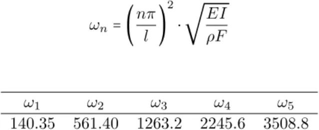
The boundary conditions for a simply supported beam are described by the equations: X(0)=
0, X′′(0)
=0, X(l)=0 andX′′(l)=0 and free vibration frequencies can be determined from
the relationship:
ωn=(
nπ l )
2
⋅
√
EI ρF
are listed in Table 1:
ω1 ω2 ω3 ω4 ω5
140.35 561.40 1263.2 2245.6 3508.8
Table 1 Five first natural frequencies of the beam before modification
It is assumed that after modification the first natural frequency have to equal to ω1=100
[1/sec].
According to the proposed algorithm the needed matrixes takes form:
A=
⎡⎢ ⎢⎢ ⎢⎢ ⎢⎢ ⎢⎢ ⎢⎣
coshλ0 sinhλ0 cosλ0 sinλ0 0
coshλ0 sinhλ0 −cosλ0 −sinλ0 0
coshλl sinhλl cosλl sinλl a35
coshλl sinhλl −cosλl −sinλl a45
coshλxa sinhλxa cosλxa sinλxa −1
⎤⎥ ⎥⎥ ⎥⎥ ⎥⎥ ⎥⎥ ⎥⎦
(6)
a35=
λ
2ρF ⋅[sinhλ(l−xa)−sinλ(l−xa)]
a45=
λ
2ρF ⋅[sinhλ(l−xa)+sinλ(l−xa)]
B=
⎡⎢ ⎢⎢ ⎢⎢ ⎢⎢ ⎣
coshλ0 sinhλ0 cosλ0 sinλ0 coshλ0 sinhλ0 −cosλ0 −sinλ0
coshλl sinhλl cosλl sinλl
coshλl sinhλl −cosλl −sinλl
⎤⎥ ⎥⎥ ⎥⎥ ⎥⎥ ⎦
(7)
where: λ4
=ρF/EI⋅(100)2
For the assumed frequency ω1, the curve ma=f(xa), representing the value of additional
mass vs. its position, was determined from the equation:
ma=detB/(detA+detB)
This curve is shown in Fig. 1.
0 0.2 0.4 0.6 0.8 1 1.2 1.4 1.6
0 10 20 30 40 50 60 70 80 90
xa ma
Figure 1 The value of additional massmavs. its positionxa
For each pair (ma, xa) on the curve showed in Fig.1 the first free vibration frequency is
equal to the desired value (ω1= 100 1/sec). Author proposes to choose the additional mass
and its position according to one of the four criteria:
1. the choice of the minimal mass;
2. the arbitrary choice of mass and determination its position;
4. such a choice of mass and corresponding position so that the vibration node of the second form of the free vibrations (mode) is placed in the desired cross-section.
The criterion of minimal mass is the most obvious criterion for choice of mass and its position. In the analyzed case, the additional mass with the value of ma = 3.78 [kg] should
be added to the beam in the cross-section with the coordinate xa = 0.8 [m]. To check the
computational model, also the calculations for the system with the additional mass were carried out with the use of the Finite Element Method.
The free vibration frequencies, determined for this mass, coming from the analytical inverse model and from the FEM, are listed in Tab. 2.
Table 2 Five first natural frequencies of the system after modification - with minimal mass ω1 ω2 ω3 ω4 ω5
102.40 574.24 1043.2 2288.6 3069.8
Using criteria No 2 and No 3 is quite obvious. They consist in arbitrary choice of the additional mass and determination of its position from Fig. 1 - criterion No 2. The criterion No 3 concerns the case when adding the mass is possible only in the given section - the mass values can be determined from Fig. 1.
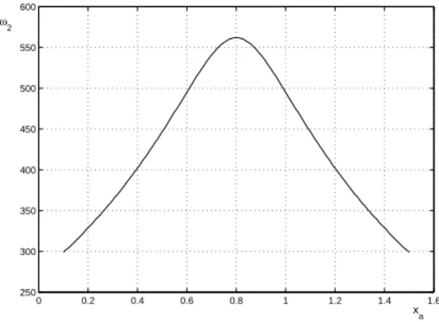
Choice of the pair (ma, xa) determinates the value of the second frequency of free vibration
and the position of vibration node of the second mode of the beam.
Graph of this frequency changes vs. position (for the corresponding value of additional mass) is shown in Fig. 2.
0 0.2 0.4 0.6 0.8 1 1.2 1.4 1.6
250 300 350 400 450 500 550 600 ω2
x
a
Figure 2 Second natural frequency as a function of the addition mass location
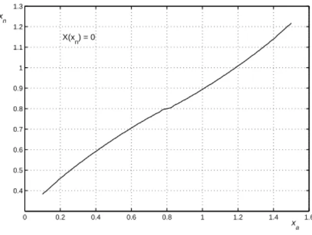
0 0.2 0.4 0.6 0.8 1 1.2 1.4 1.6 0.4
0.5 0.6 0.7 0.8 0.9 1 1.1 1.2 1.3
x
a
x
n
X(x
n) = 0
Figure 3 Position of the second eigenmode node as a function of the additional mass location
If, in the discussed case, not only the given value of the first frequency ω1 is desired, but
the vibration node of the second mode has to be in the section with coordinate xn = 1 [m],
then one should choose the additional mass position, according these criteria and on the basis on the characteristic shown on Fig. 3, as xd =1.26[m]. Next, the additional mass with the
value ofma=6.05 [kg] is selected on the basis on the characteristic shown on Fig. 1
To check the correctness of the model, the calculations (for the determined values) with the help of the FEM were carried out. Frequencies, determined in the analysis, are listed in Table 3.
Table 3 Five first natural frequencies of the system ω1 ω2 ω3 ω4 ω5
102.4 409.5 1100.6 2213.3 3537.1
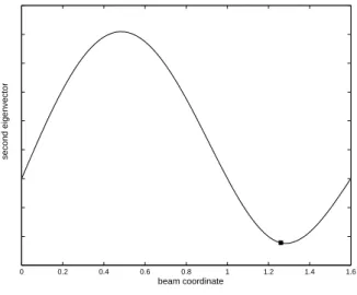
The second mode of the free vibrations, determined from the FEM analysis, is shown in Fig. 4. The square marks the additional mass position.
Of course, the node position does not depend on the mass value. This allows to determinate of such its position so that the vibration node of the second form of the free vibrations occurs in a given section, first, and next to select such a value of mass ma so that the desired first
frequency is achieved.
Taking into account free vibration frequencies of the system after modification, listed in Tab. 2 and Tab. 3, one can see that selection of mass with the accuracy 0.01 kg causes that the first free-vibration frequency differs from the desired value by about 2%.
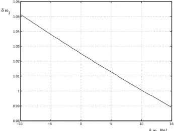
Influence of the uncertainties of mass and its position, correspondingly, determination on the free vibration frequency is shown in Fig. 5.
0 0.2 0.4 0.6 0.8 1 1.2 1.4 1.6
beam coordinate
second eigenvector
Figure 4 Second eigenmode of beam
i.e. such a value for which the curve in Fig. 5a achieves the value 1. This is mass that should be added to the beam in the section with coordinatex=0.8[m] to cause that the first free-vibration frequency of the system after modification is equal to the desired frequency, i.e.
ω1=100[1/sec].
5.2 Cantilever beam - increasing of free vibration frequencies
For cantilever beam boundary conditions are described by equations: X(0) = 0, X′(0)=0, X′′(l)
= 0 i X′′′(l) = 0. Natural frequencies for beam with data as in previous example in
Table 4 are listed:
Table 4 Five first natural frequencies of the cantilever beam ω1 ω2 ω3 ω4 ω5
50.0 313.4 877.4 1719.3 2842.1
It is assumed that after modification the first natural frequency has to equal toω1 = 100 [1/s].
In order to find the value of elastic support coefficient the proposed algorithm is used. The matrixes from proposed algorithm have the forms:
A=
⎡⎢ ⎢⎢ ⎢⎢ ⎢⎢ ⎢⎢ ⎢⎣
coshλ0 sinhλ0 cosλ0 sinλ0 0
sinhλ0 coshλ0 −sinλ0 cosλ0 0
coshλl sinhλl −cosλl −sinλl a35
sinhλl coshλl sinλl −cosλl a45
coshλxs sinhλxs cosλxs sinλxs −1
⎤⎥ ⎥⎥ ⎥⎥ ⎥⎥ ⎥⎥ ⎥⎦
(8)
−10 −5 0 5 10 15 0.98
0.99 1 1.01 1.02 1.03 1.04 1.05 1.06
δ ma [%] δ ω1
(a) Influence of uncertainties of mass value determination
0.7 0.72 0.74 0.76 0.78 0.8 0.82 0.84 0.86 0.88 0.9 1
1.002 1.004 1.006 1.008 1.01
xa [m] δ ω1
(b) Influence of uncertainties of mass position determina-tion
Figure 5 Influence of uncertainties of mass value and its position determination on natural frequency
a35=−
1
2EIλ3 ⋅[sinhλ(l−xs)+sinλ(l−xs)]
a45=−
1
B= ⎡⎢ ⎢⎢ ⎢⎢ ⎢⎢ ⎣
coshλ0 sinhλ0 cosλ0 sinλ0 sinhλ0 coshλ0 −sinλ0 cosλ0
coshλl sinhλl −cosλl −sinλl
sinhλl coshλl sinλl −cosλl
⎤⎥ ⎥⎥ ⎥⎥ ⎥⎥ ⎦
(9)
where: λ4
=ρF/EI⋅(100)2
Matrix B comes from the matrix A through crossing the last row and the last column
off. So, the matrix B is a matrix describing the eigenvalue problem for a beam without an additional element.
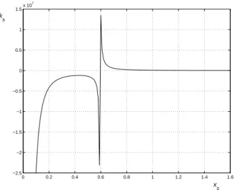
From equation:
ks=detB/(detA+detB)
the curve representing the value of support elasticity vs. support position is determined. This curve is shown in Fig. 6
0 0.2 0.4 0.6 0.8 1 1.2 1.4 1.6
−2.5 −2 −1.5 −1 −0.5 0 0.5 1 1.5x 10
7
ks
xs
Figure 6 Support elasticityksas a function of support locationxs
Similar like in case of additional mass, for each pair (ks, xs) on the curve showed in Fig.6
the first free vibration frequency is equal to the desired value i.e. (ω1=100 rad/sec).
Choice of the value of support elasticity and its position can be made according to one of the criteria:
1. the choice (if possible) of the rigid support (ks→∞);
2. supporting the beam with a system with positive coefficient of elasticity
• the arbitrary choice of elasticity (from the possible values) and determination of the
• the arbitrary choice of the support position and determination of corresponding
elasticity;
3. supporting the beam with a system with negative coefficient of elasticity
• the arbitrary choice of elasticity (from the possible values) and determination of the
support position;
• the arbitrary choice of the support position and determination of corresponding
elasticity;
The easiest task for technical realization seems to be supporting the beam with the rigid support. The beam should be supported in the section where the coefficient ks →∞. In the
analyzed case, this is the section with coordinate xs=0.6[m].
To check correctness of the proposed inverse model algorithm, the free vibration frequencies for a beam with a rigid internal support were determined using Finite Elements Method. The results are presented in Tab. 5.
Table 5 Five first natural frequencies of the beam with internal right support ω1 ω2 ω3 ω4 ω5
103.24 687.35 1728.9 2286.99 4087.53
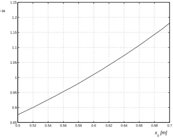
Influence of the uncertainties of rigid support position on the first (modified) free vibration frequency is shown in Fig.7.
0.5 0.52 0.54 0.56 0.58 0.6 0.62 0.64 0.66 0.68 0.7 0.85
0.9 0.95 1 1.05 1.1 1.15 1.2 1.25
xs [m] δ ω
Figure 7 The change of first natural frequency as a function of support location
special system with negative coefficient of elasticity. More information about the systems with negative coefficient of elasticity can be found in [8].
With the assumption that the beam can be supported in the section with coordinatex=1m, the coefficient of elasticity amount toks=68.6 ⋅ 103[N/m].
The free vibration frequencies of the so supported beam, determined with the use of FEM, are listed in Tab.6.
Table 6 Five first natural frequencies of the beam after modification ω1 ω2 ω3 ω4 ω5
103.62 336.61 902.25 1752.56 2892.07
Influence of the uncertainties in the determined elasticity and support coordinate values on the difference between the desired and determined free frequency value, correspondingly, is shown in Fig. 8.
5.3 Cracks diagnostics
The calculations were carried out for the beam with data: lengthl=0.1m, heighth=0.0016m, width b = h, densityρ = 7960 kg/m3
, Young’s modulus E=2.1⋅1011 Pa and Poisson ratio ν = 0.3 [11]
5.3.1 Simply supported beam
In case of simply supported beam, boundary conditions are described by equationsX(0) = 0, X′′(0)
= 0, X(l) = 0 and X′′(l) = 0.
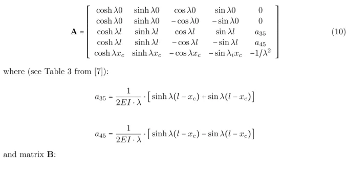
Matrix A from proposed above algorithm has form:
A=
⎡⎢ ⎢⎢ ⎢⎢ ⎢⎢ ⎢⎢ ⎢⎣
coshλ0 sinhλ0 cosλ0 sinλ0 0
coshλ0 sinhλ0 −cosλ0 −sinλ0 0
coshλl sinhλl cosλl sinλl a35
coshλl sinhλl −cosλl −sinλl a45
coshλxc sinhλxc −cosλxc −sinλixc −1/λ2
⎤⎥ ⎥⎥ ⎥⎥ ⎥⎥ ⎥⎥ ⎥⎦
(10)
where (see Table 3 from [7]):
a35=
1
2EI⋅λ⋅[sinhλ(l−x
c)+sinλ(l−xc)]
a45=
1
2EI⋅λ⋅[sinhλ(l−x
c)−sinλ(l−xc)]
0.9 0.95 1 1.05 1.1 0.96
0.98 1 1.02 1.04
δ ω
δ ks
(a) Influence of elasticity determination
0.9 0.95 1 1.05 1.1
0.85 0.9 0.95 1 1.05 1.1
δ ω
xs
(b) Influence of support location
Figure 8 Influence of the uncertainties in the determined elasticity and support coordinate on first natural frequency of the beam
B=
⎡⎢ ⎢⎢ ⎢⎢ ⎢⎢ ⎣
coshλ0 sinhλ0 cosλ0 sinλ0 coshλ0 sinhλ0 −cosλ0 −sinλ0
coshλl sinhλl cosλl sinλl
coshλl sinhλl −cosλl −sinλl
⎤⎥ ⎥⎥ ⎥⎥ ⎥⎥ ⎦
(11)
This matrix has identical form lake main matrix for boundary problem of beam without crack.
cb=
detB
detA+detB (12)
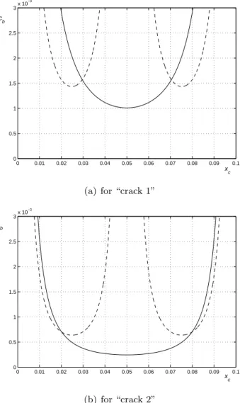
Function of one variable is obtained in this way for every free vibration frequency (the inverse model in ambiguous). Thus, one needs at least two free vibration frequencies. The crossing point of the cb vs. xc curves for two different free-vibration frequencies determines
the searched crack parameters.
In figure 9a and 9b curves cb=f(xc) for two first natural frequency of simply supported
beam with two different cracks (data from [11]) are showed.
0 0.01 0.02 0.03 0.04 0.05 0.06 0.07 0.08 0.09 0.1 0
0.5 1 1.5 2 2.5
3x 10
−3
x c c
b
(a) for “crack 1”
0 0.01 0.02 0.03 0.04 0.05 0.06 0.07 0.08 0.09 0.1 0
0.5 1 1.5 2 2.5
3x 10
−3
x c c
b
(b) for “crack 2”
Figure 9 Curves flexibilitycg as function of crack locationxp
In fig. 9 continuous line marked curve, which is obtained for frequency f1 and dashed line
which side of beam centre is crack one should carry out with other methods.
Comparison of crack parameters identified and modeled in FEM for cases: “crack 1” and “crack 2” are showed in Tab. 7.
Table 7 Identification of crack
crack FEM model natural frequencies [Hz] identification error
“1” xc=70mm f1=370.31 f2=1475.36 xc=70.4 0.6%
a=0.3⋅h a=0.303⋅h 1.0%
“2” xc=80mm f1=371.93 f2=1481.52 xc=80.9 1.25%
a=0.2⋅h a=0.205⋅h 2.5%
Graphs of flexibilitycbas a function of crack positionxcfor free vibration frequencies, with
the measurement uncertainties taken into account, are shown in Fig.10. The errors δ1 and δ2
were determined from comparison of the free vibration frequencies of the beam without crack modeled by FEM ω0i−F EM and the frequencies obtained for the analytical model ω0i−A:
δi=∣ω0i−M ES−ω0i−A∣/ω0i−A
Graphs of the searched curves for four frequencies ω1±δ1 and ω2±δ2 for the case “crack
2” in the vicinity of crack position xc=80mm are shown in Fig. 10.
0.0722 0.074 0.076 0.078 0.08 0.082 0.084 4
6 8 10 12 14 16x 10
−4
c
b
x
c
Figure 10 Flexibilityc
bas a function ofxcfor frequencies “determined” with an error
Solid lines mark the curves determined for ω1±δ1, while the dotted ones – the curves
determined forω2±δ2. The identified values of crack position and its depth are situated in the
common part of the interiors of the regions bounded with the curves determined by solid lines and by dotted lines. This region defines position of the crack in the interval xc∈(75−83)mm
and its depth in the intervala∈(0.15−0.26)⋅h (the modeled parameters arexc=80mm and
5.3.2 Cantilever beam
In case of cantilever beam main matrixA has a form:
A= ⎡⎢ ⎢⎢ ⎢⎢ ⎢⎢ ⎢⎢ ⎢⎢ ⎢⎢ ⎢⎢ ⎢⎢ ⎢⎣
1 0 1 0 0
0 1 0 1 0
coshλil sinhλil −cosλil −sinλil a35
sinhλil coshλil sinλil −cosλil a45
coshλixc sinhλixc −cosλixc −sinλixc −1/λ2i
⎤⎥ ⎥⎥ ⎥⎥ ⎥⎥ ⎥⎥ ⎥⎥ ⎥⎥ ⎥⎥ ⎥⎥ ⎥⎦ where:
a35=
1 2λi ⋅
EI⋅[sinhλi(l−xc)−sinλi(l−xc)];
a35=
1 2λi
⋅EI⋅[coshλi(l−xc)−cosλi(l−xc)]
And matrix B:
B= ⎡⎢ ⎢⎢ ⎢⎢ ⎢⎢ ⎢⎢ ⎢⎢ ⎢⎢ ⎢⎢ ⎢⎣
1 0 1 0
0 1 0 1
coshλil sinhλil −cosλil −sinλil
sinhλil coshλil sinλil −cosλil
⎤⎥ ⎥⎥ ⎥⎥ ⎥⎥ ⎥⎥ ⎥⎥ ⎥⎥ ⎥⎥ ⎥⎦
This matrix have identical form lake main matrix for boundary problem of beam without crack.
Natural frequencies of cantilever beam, necessary to identification came from FEM analyses. Geometrical and material parameters of beam are the same as in previous example. Author has examined 6 different variants of crack parameters. Identification results of are showed in Table 8
Graphs of the searched curves for four frequencies ω1±δ1 and ω2±δ2 for the case “crack
4” in the vicinity of crack position xc = 80mm are shown in Fig.11. Errors δ1 and δ2 was
determined as in previous example.
Solid lines mark the curves determined for ω1±δ1, while the dotted ones - the curves
determined forω2±δ2. The identified values of crack position and its depth are situated in the
Table 8 Identification of crack
crack FEM model natural frequencies [Hz] identification error
“1” xc=10 f1=132.41 f2=834.07 xc=8.94 10.6%
a=0.2⋅h a=0.189⋅h 5.5%
“2” xc=10 f1=131.07 f2=830.57 xc=8.91 10.9%
a=0.3⋅h a=0.274⋅h 8.7%
“3” xc=30 f1=133.04 f2=835.45 xc=32.2 7.3%
a=0.2⋅h a=0.208⋅h 4.0%
“4” xc=30 f1=132.44 f2=834.20 xc=31.6 5.3%
a=0.3⋅h a=0.283⋅h 5.7%
“5” xc=50 f1=133.40 f2=832.32 xc=49.3 1.4%
a=0.2⋅h a=0.189⋅h 5.5%
“6” xc=50 f1=133.32 f2=827.33 xc=53.6 7.2%
a=0.3⋅h a=0.264⋅h 12.0%
0.0260 0.028 0.03 0.032 0.034 0.036 0.038 0.04 0.042 0.044 0.5
1 1.5 2 2.5 3 3.5 4 4.5
5x 10
−3
c
b
x
c
Figure 11 Flexibilitycbas a function ofxpfor frequencies “determined” with an error
and its depth in the intervala∈(0.22−0.378)⋅h (the modeled parameters arexc=30mm and
a=0.3⋅h).
6 SUMMARY AND CONCLUSIONS
In the work, the problems of the beam structural modification through coupling the additional point mass or elastic support, as well as the problem of diagnostics of the beam cracks, were discussed.
support in one point, crack described as joint). This allows describing vibrations of such system with the use of generalized functions, thanks to what the mathematical description of vibrations in each problem has the same form.
In order to solve the inverse problem, i.e. the problem of finding values of the additional quantities (mass, elasticity), the beam inverse model was proposed. Analysis of this model allows finding such a value of additional mass (elasticity) as a function of its localization so that the free vibration frequency changes to desirable value, when such mass is coupled to the beam. The criteria for choice of the “proper” pair (mass - its position), including the criterion allowing changing the position of the vibration node of the second form of the free vibrations (or of arbitrary another one) (retaining the desired value of the first free vibration frequency), were given.
Analysis of the influence of uncertainties in the determination of the additional quantity value and its position on the desired free vibration frequency was carried out, too. With 10% errors in determination of this quantity and its position assumed, the errors of the desired frequency did not exceed 5%.
The proposed beam inverse model can be employed to identify of the beam cracks. In such a case, however, the input quantity is free vibration frequency measured on the damaged object.
Each determined free-vibration frequency allows determining the flexibility curve for the spring modeling crack as a function of its position. For each pair of parameters (cb, xc) lying
on the curve, the free vibration frequency is equal to the frequency measured. The searched parameters of the crack lay in the point that is common for two arbitrary curves.
Accuracy of crack parameters (its depth and position) determination depends on accuracy (uncertainty) of frequency measurement. Only some regions containing the searched crack parameters can be obtained in such a situation. In extreme cases, these regions can contain the whole length of the beam. The identification errors can be decreased by increasing number of the determined free-vibration frequencies. For instance, for five determined frequencies, ten pairs of curves are obtained and next, after statistical processing, one can determine the searched crack parameters.
References
[1] F. Aryana and H. Bahai. Sensityvity analysis and modification of structural dynamic characteristic using second order approximation. Engineering Structures, 25:1279–1287, 2003.
[2] H. Bahai, K. Farahani, and M.S. Djoudi. Eigenvalue inverse formulation for optimising vibratory behaviour of truss and continuous structures. Computers and Structures, 80:2397–2403, 2002.
[3] M.S. Djoudi, H. Bahai, and I.I. Esat. An inverse eigenvalue formulation for optimising the dynamic behaviour of pin-joined structures. Journal of Sound and Vibration, 253:1039–1050, 2002.
[4] G. Gladwell. Inverse problem in vibration. Kluwer Academic, 2nd edition, 2004.
[5] L. Majkut. Crack modeling in vibroacoustic model based diagnostics. Diagnostyka, 34:15–22, 2005. (in polish).
[6] L. Majkut. Acoustical diagnostics of cracks in beam like structures. Archives of Acoustics, 31:17–28, 2006.
[8] http://www.minusk.com.
[9] J.E. Mottershed, A. Kyprianu, and H. Ouyang. Structural modification. Part 1: rotational receptances. Journal of Sound and Vibration, 284:249–265, 2005.
[10] J.E. Mottershed, M.G. Tehrani, D. Stancioiu, S. James, and H. Shahverdi. Structural modification of a helicopter tailcone.Journal of Sound and Vibration, 298:366–384, 2006.