SRef-ID: 1432-0576/ag/2004-22-1177 © European Geosciences Union 2004
Annales
Geophysicae
Simultaneous HF measurements of E- and F-region Doppler
velocities at large flow angles
R. A. Makarevitch1, F. Honary1, and A. V. Koustov2
1Department of Communication Systems, Lancaster University, Lancaster, LA1 4YR, UK
2Institute of Space and Atmospheric Sciences, University of Saskatchewan, 116 Science Place, Saskatoon, SK, S7N 5E2,
Canada
Received: 3 June 2003 – Revised: 30 October 2003 – Accepted: 5 November 2003 – Published: 2 April 2004
Abstract.Data collected by the CUTLASS Finland HF radar are used to illustrate the significant difference between the cosine component of the plasma convection in the F-region and the Doppler velocity of the E-region coherent echoes observed at large flow angles. We show that the E-region velocity is ∼5 times smaller in magnitude and rotated by ∼30◦ clockwise with respect to convection in the F-region. Also, measurements at flow angles larger than 90◦ exhibit a completely new feature: Doppler velocity increase with the expected aspect angle and spatial anticorrelation with the backscatter power. By considering DMSP drift-meter mea-surements we argue that the difference between F- and E-region velocities cannot be interpreted in terms of the con-vection change with latitude. The observed features in the ve-locity of the E-region echoes can be explained by taking into account the ion drift contribution to the irregularity phase ve-locity as predicted by the linear fluid theory.
Key words. Ionosphere (auroral ionosphere; ionospheric ir-regularities; plasma convection)
1 Introduction
The auroral ionosphere is filled with the magnetic-field-aligned irregularities that can be detected by coherent radars (Fejer and Kelley, 1980; Haldoupis, 1989; Sahr and Fe-jer, 1996; Schlegel, 1996). At the F-region heights (above 130 km) these irregularities are believed to move with the velocity of plasma convection,V0=E×B/B2. Thus, the
ve-locity of irregularity motion in the F-region is a measure of the electric field applied to the ionosphere. At the E-region heights of 100–120 km the irregularity velocity depends on several parameters; among the most important ones are the electric field magnitudeEand the angles that the irregular-ity propagation vectorkmakes with the electron background driftVe0(flow angleθ) and magnetic fieldB (the
comple-mentary off-perpendicular angle is called the aspect angleα).
Correspondence to:R. A. Makarevitch ([email protected])
In the E-region, the electron background driftVe0to a good
approximation equals the convection velocity in the F-region,
Ve0∼=V0, since the electric field does not change
signifi-cantly along the highly conductive magnetic field lines. A number of recent studies successfully exploited the de-scribed above electrical link between the F and E-regions, to study the velocity of the E-region irregularities as a function of the ionospheric electric field. In the UHF band, Foster and Erickson (2000), in a unique subauroral experiment, stud-ied the E-region Doppler velocity detected with the side lobe of the incoherent radar at Millstone Hill (440 MHz) in con-junction with the F-region electric field data from the radar’s main lobe on the same magneticLshell. These authors dis-covered an almost perfect linear relationship between the E-region Doppler velocity and the electric field magnitude. In the VHF band, a comparison between F-region drifts ob-served by the European Incoherent Scatter (EISCAT) radar and the Doppler velocities measured by the Scandinavian Twin Auroral Radar Experiment (STARE) VHF radars (140 MHz) showed that the irregularity phase velocity for di-rections close to Ve0 (θ=0◦−60◦) is significantly smaller
than the projection of Ve0 onto the line-of-sight (l-o-s),
Vlos=Ve0cosθ, while for larger flow anglesθ=60◦–90◦, the
10
20 30
65 70 0
1 2
3 4 5 6
7 8
9 10 11 12 13 14 15
765 km
0 75 150 225 300 375 450 525 600 675 750 -VF, m/s
0 20 40 60 80 100 120 140 160 180 200 -VE
630 km 900 km
1035 km 1215 km
L= 600 L= 650
L= 700 1000 m/s
0 1 2
360 km
270 km
F13
F12
495 km
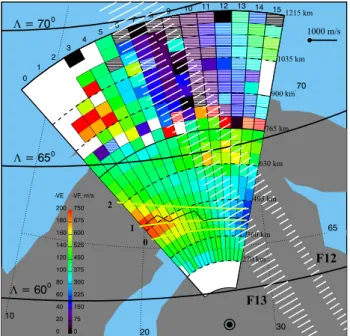
Fig. 1.Field of view plot of the averaged Doppler velocity observed by the CUTLASS Finland radar during the interval 14:40–14:50 UT on 31 March 2000. Each radar cell is color coded according to the color bar shown in the left bottom part of the diagram. The color scheme forr=180−765 km (r=765−1215 km) is indicated by the digits to the left (right) of the color bar. The echoes in cells filled by the horizontal lines have, on average, positive velocities corre-sponding to the color of the line. Also shown are slant range marks (dashed circular curves) and PACE lines of equal magnetic latitudes
3=60◦, 65◦, and 70◦(solid thick curves). Thick yellow curves 0–2 denote the off-perpendicular (aspect) angle lineα=0◦(see text for details). Thin ragged solid black line shows the location of the av-erage power maxima along each radar beam. Two DMSP passes (F13: 14:43–14:48 UT and F12: 17:05–17:10 UT) with the mea-sured perpendicular ion velocities are indicated by white vectors. The scale for the ion velocities is shown in the top right corner of the diagram.
Simultaneous observations of E-region velocities at HF and F-region plasma drifts are difficult to perform since cur-rently available HF radars are positioned too far equatorward from the incoherent radar locations. In this respect, an inter-esting approach was undertaken by Milan and Lester (1998), who compared the CUTLASS Iceland E-region Doppler ve-locities with the F-region drifts measured by the same radar 100–200 km poleward and eastward of the E-region scatter area. The authors found that the average E-region velocity, at small flow angles was well below the l-o-s component of the F-region velocity though still correlated with it.
In this study we expand the approach of Milan and Lester (1998) with the goal to explore the relationship between the E-region HF Doppler velocity and the plasma drift in the F-region at large flow angles. Earlier studies by Makarevitch et al. (2002a, b) and Milan et al. (2003) have indicated that the cosine law might not be appropriate at HF even at large flow angles, but the results were not well substantiated in the sense
that no reliable convection measurements were available. In this study we use F-region convection measurements by the CUTLASS Finland HF radar supported by the Defence Me-teorological Satellite Program (DMSP) data on the ion drift velocities in the upper F-region and compare them with the E-region Doppler velocity measurements.
2 Observations
The CUTLASS Finland HF radar (62.3◦N, 26.6◦E), to-gether with the Iceland HF radar, forms the easternmost part of the Super Dual Auroral Radar Network (SuperDARN) system of paired coherent HF radars and is designed to mon-itor the large-scale convection patterns at F-region heights in the high-latitude ionosphere (Greenwald et al., 1995). The radar is agile in frequency (8–20 MHz) and measures the Doppler velocity, backscatter power and width of iono-spheric echoes in 45-km steps (180–3500 km) for each of the 16 radar beam positions separated by 3.24◦in azimuth. Beam 0 (15) of the radar corresponds to the westernmost (eastern-most) direction.
We concentrate in this study on a four-hour interval be-tween 13:30 and 17:30 UT on 31 March 2000. During this event, from 13:30 UT to 16:30 UT, the radar observed a sta-ble band of E-region echoes at slant rangesr=350–750 km. After 16:30 UT the echoes became weaker, the band nar-rowed (r=400–600 km) and eventually disappeared. During almost entire period (13:40–17:10 UT), the radar observed simultaneously F-region echoes at farther rangesr>750 km. Co-existence of the E- and F-region echoes, even in spatially separated areas, provided an opportunity for velocity com-parisons in the E- and F-regions, because DMSP measure-ments during the period under study did not indicate sig-nificant latitudinal variation of the convection intensity, as shown below.
Throughout the period the IMF was very stable and south-ward, Bz=−3 nT; By=−5 nT; the Kp index was also
sta-ble and around 3. The level of ionospheric absorption and magnetic perturbations as measured by the IRIS imaging ri-ometer at Kilpisjarvi (69.1◦N, 20.8◦E) and magnetometers of the IMAGE and SAMNET networks of high-resolution fluxgate magnetometers within the radar near FoV, was low, 0.1–0.2 dB and 100–250 nT, respectively, and exhibited lit-tle variation with time, indicating that the ionosphere was in a quite stable state. Under the above conditions one would expect that the convection pattern consists of 2 global cells with the stable L-shell-aligned flow in the afternoon sec-tor of the magnetosphere (MLT∼=UT+2 for the radar FoV). Indeed, the SuperDARN global convection maps (not pre-sented here) based on the Ruohoniemi and Baker (1998) technique demonstrate the high degree ofL-shell alignment of the flow for the interval under study and latitudes of inter-est.
indicated in Fig. 1 by black curves. In addition, Fig. 1 presents ion drift data for two DMSP passes over the radar near FoV during the interval under study. The vector length at each point of the path corresponds to the measured ion ve-locity perpendicular to the path. The scale for the ion veve-locity is indicated in the top right corner of the diagram. Data from an DMSP altitude of 810 km were projected to the E-region height of 110 km along the magnetic field line. The Doppler velocity averaged over a 10-min interval, 14:40–14:50 UT (corresponding to the first pass of DMSP), is indicated by the color according to the scheme given in the left bottom part of the diagram as a color bar. The velocity scale for ranges 180–765 km (765–1215 km) is indicated by the digits to the left (right) of the color bar. Cells filled with horizontal lines correspond to the positive velocities. The slant range marks of 270, 360, 495, 630, 765, 900, 1035, and 1215 km are indicated by the dashed circular lines. We also show, by yellow curve 0, the line of perfect aspect angle at 110-km altitude (α=0), assuming that the radar rays undergo refrac-tion based on typical ionospheric profiles, as described by the model (Bilitza, 2001) and using a simple geometric op-tics approach (Uspensky et al., 1994). Curves 1 and 2 rep-resent the zero aspect angle for the electron density reduced by 25% and 50%, respectively. Finally, the thin ragged solid black line close to the yellow curve 1 shows the location of the power maxima along each radar beam.
An important feature of the F-region echoes detected at farther ranges (r=765−1215 km) is their negative velocities up to−750 m/s in the western part of the FoV and positive velocities up to +500 m/s in the eastern part of the FoV. The change in the Doppler velocity sign occurs at beams 9–10, corresponding to the direction nearly perpendicular to magnetic L shells, which is indicative of the L -shell-aligned nature of the flow at far ranges. At closer ranges (r=180−765 km), where E-region echoes were detected, no reversal of the velocity sign is observed. The E-region ve-locity magnitude is maximized for beam 0 (red area with
V=200 m/s). It gradually decreases to 50 m/s (blue area) with the beam number increase being still negative for beam 15. The range location of the power maxima (the black ragged line in Fig. 1) follows closely the aspect angle curve 1. Since it is widely accepted that the echo power should be at maximum for the range of perfect aspect angle (Fejer and Kelley, 1980; Haldoupis, 1989; Sahr and Fejer, 1996), from hereafter we take the curve 1 from Fig. 1 as a model for the aspect angle within the radar FoV.
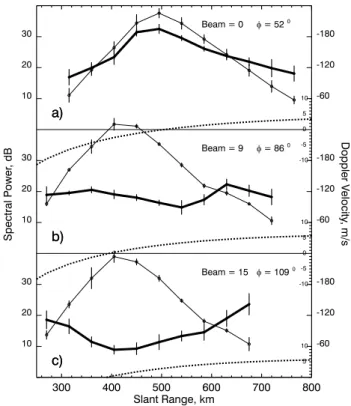
Curiously enough, in Fig. 1 at beams 13–15 the velocity magnitude is smaller atr=360−495 km, close to the range of the perfect aspect angle, as opposed to the velocity mag-nitudes at beams 0–5, where it is clearly at maximum at
r∼=495 km. To make this point clearer, we present the data of Fig. 1 using a different format. The solid thick (thin) curve in Fig. 2 shows the averaged (for the 14:40–14:50 UT interval) Doppler velocity (backscatter power) slant range profiles for beams 0, 9, and 15. For slant ranges 270–765 km the aver-agedL-shell angleφ, defined as the angle between the radar look direction and theL-shell direction in the western
sec-300 400 500 600 700 800
Slant Range, km
DopplerV
elocity
,m/s
SpectralP
ower
,dB
c)
c) 5
10
Beam = 15 f= 1090
10 20 30
-60 -120 -180 b)
b) 5
10
0
-10 -5
Beam = 9 f= 860
10 20 30
-60 -120 -180 a)
a) 5
10
0
-10 -5
Beam = 0 f= 520
10 20 30
-60 -120 -180
Fig. 2.Slant range profiles of echo power (thin solid line), Doppler velocity (thick solid line), and aspect angle (dotted line), for CUT-LASS beams 0, 9, and 15 for 31 March 2000, 14:40–14:50 UT. Scale for aspect angle is indicated on the right vertical axis by small ticks with zero aspect corresponding to horizontal lines at the bottom of each panel. The averaged for slant ranges 270–765 km
L-shell angleφfor each beam is shown in the right top corner of each panel.
tor (assumed direction of the plasma flow), is given in the right top corner of each panel. The scale for the backscatter power (Doppler velocity) is shown on the left (right) vertical axis. Also shown by a dotted line is the model aspect angle
αas a function of slant range for each beam. The scale for aspect angle in degrees is given by small ticks±10,±5,0 on the right axis. One can notice that for each radar look-direction the average echo power has a clear maximum at a range r0 corresponding closely to the range with perfect
aspect angle,α(r0)=0. The velocity magnitude profile for
beam 0 shows quite a similar slant range variation with max-imum atr0. However, in beam 15 there is no maximum of
velocity atr0, but distinct minimum. At intermediate beam
9 the velocity change with slant range is not strong, with weakly-pronounced local minimum and maximum at 540 and 630 km, respectively (both not atr0).
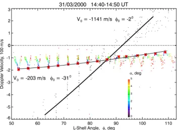
To explore this effect in more detail we present the same data using a different approach developed by Makarevitch et al. (2002b). Figure 3 shows the Doppler velocity versus
31/03/2000 14:40-14:50 UT
50 60 70 80 90 100 110
L-Shell Angle,f, deg -6
-5 -4 -3 -2 -1 0 1 2 3
0
DopplerV
elocity
,100m/s
0 1 2 3 4 5
a, deg
V0= -1141 m/s f0= -2 0
V0= -203 m/s f0= -31 0
Fig. 3. Scatter plot of the Doppler velocity versusL-shell angle
φ for 31 March 2000, 14:40–14:50 UT. The points correspond-ing to E-region scatter are color coded in aspect angleα, as in-dicated in the bottom right part of the diagram. The red crosses are maxima/minima of the averaged velocity along radar beams, as described in the text. The F-region velocities are shown by black points. The solid thin (thick) line represents the best fit,
V0cos(φ+φ0), to red crosses (all black points).
aspect angle is shown at the bottom right part of the diagram. One can notice right away that F- and E-region echoes ex-hibit strikingly different velocity variations with theL-shell angle. The F-region echoes are steadily increasing in veloc-ity from negative to positive values withL-shell angle; the reversal of the velocity sign occurs atφ∼=90◦. The E-region echoes are also progressively less negative withφincrease, but no reversal in velocity sign occurs.
One of the most remarkable features of the E-region points is the presence of V-like structures. For example, the Doppler velocity first increases in magnitude for φ=51◦−53◦ and then decreases forφ=53◦−56◦with the smaller aspect angle points at the bottom of V-structure. We interpret this feature as associated with the aspect angle attenuation of the phase velocity (Makarevitch et al., 2002b). Each V-structure is in fact the data from one of the radar beams. As the range and
L-shell angle changes along the beam, so does the aspect an-gle, reaching at some range minimum where the phase veloc-ity is expected to have maximum. The V-structures in Fig. 3 are thus just another form of the Fig. 2a presentation. For high-number beams, for example, beam 15, the inverse-V-or3-structures are seen instead, with the good aspect angle points at the top of the3-structures, which is rather unex-pected but in agreement with the presentation of Fig. 2c (we return to the interpretation of this feature in Sect. 3). The V-or3-structures are not recognizable in the middle part of the diagram because theL-shell angle does not change much for the central beams. Only points at the bottom (top) of V- (3-) structures marked by the red crosses should be considered when comparingL-shell angle dependencies in the E- and F-regions, since all other points are significantly affected by the aspect angle attenuation. To facilitate such a comparison we
31/03/2000 13:40-17:10 UT
1340 1400 1420 1440 1500 1520 1540 1600 1620 1640 1700 Universal Time
-12 -10 -8 -6 -4 -2 0
FittedV
elocityV
0
,100m/s
-50 -40 -30 -20 -10 0 10
FittedL
-ShellAngle
f
0,deg
Fig. 4. Time variation of the fitted velocityV0(blue) andL-shell angleφ0(red) during the considered period. The scale for the
fit-ted velocity (L-shell angle) is shown on the left (right) axis. Thin (thick) line represents the results of fitting for E- (F-) region. Verti-cal thin (thick) black lines show the span (minimum to maximum) of the DMSP measurements of the ion drift in the latitudes corre-sponding to E- (F-) region for the two passes over the FoV shown in Fig. 1.
fitted two cosine law functions of the formV0cos(φ+φ0)
to the E-region data (considering only red crosses) and F-region data (all black dots), shown in Fig. 3 by the thin and thick line, respectively. The fitted parameters, velocity V0
andL-shell angle φ0, signify the flow velocity and
devia-tion of the flow from theL-shell direction, respectively. One should note here that in the above cosine model the fitted velocityV0is assumed to be negative, simply to reflect
pre-dominantly negative Doppler velocities in our observations, so that a negative flow velocityV0atφ=0 implies westward
(away from the radar) convecting plasma.
One can notice that in the F-region the flow is indeed highly L-shell-aligned, φ0=−2◦. It is not true, however,
for the E-region; the L-shell angle of the velocity reversal is shifted about 31◦ to the east from the perpendicular di-rectionφ=90◦, so that the azimuthal difference between di-rections of the flow in the F and E-regions is quite large, −2◦−(−31◦)=29◦, and so is the ratio between fitted veloci-ties 1141/203∼=5.5.
In Fig. 4 we further investigate the relationship between the E-region velocity and the F-region plasma drift by show-ing the fitted velocitiesV0(blue) andL-shell anglesφ0(red)
in the E (thin line) and F-regions (thick line) as a function of time for 10-min intervals during the entire period of inter-est, 13:40–17:10 UT. Also shown are the spans (minimum to maximum) of the DMSP ion drifts for the two passes over the radar FoV. Again, thick (thin) line represents measurements for the latitudes that correspond to the F- (E-) scatter region. One can estimate that the obtained ratio of∼5 is very typical for the entire period under study.
3 Discussion
the F- and E-region scatter areas were separated spatially by 300–400 km in our observations (Fig. 1), it is possible that it is the electric field (that mainly determines the Doppler velocity) at latitudes of the E-region observations that was smaller in magnitude and rotated by some angle with respect to that at latitudes of the F-region observations. However, the DMSP measurements of the F-region ion drifts presented in Fig. 1 do not support this scenario, at least in terms of the convection magnitude. One can see that the DMSP ion veloc-ity does not change much in a broad range of latitudes. There is perhaps a 20% reduction in the ion drift at latitudes of the E-region observations, but one cannot expect the decrease in the velocity magnitude of several times. It is impossible to say whether this reduction was due to slight convection ro-tation or a simple decrease in the magnitude. Because the DMSP drift (one component of the ion drift vector) does not change much from one point to another, we believe that no significant changes in the direction of the total ion drift vec-tor were taking place. Thus, the convection magnitude at ranges of the E-region observations is comparable to the one measured at the ranges of F-region scatter, Figs. 1 and 4. In support of our conclusion, we would like to stress the fact that our convection estimates from the CUTLASS data are in good agreement with DMSP ion drifts at ranges of F-region observations, Fig. 4. The CUTLASS/DMSP comparisons for two passes give us confidence that the convection estimates for the ranges of E-region observations and other periods are also reliable.
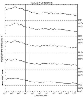
The region of interest was also monitored by several sta-tions of the IMAGE magnetometer network located within the CUTLASS near FoV. The IMAGE magnetometers mea-sure the north (X), east (Y), and vertical (Z) components of magnetic field perturbations with 10-s resolution. Figure 5 is the magnetogram of the IMAGE X-component (1X) for five IMAGE stations located along the CUTLASS beam 8. On the right axis we indicated the station three-letter abbre-viations and geographic latitudes and longitudes. One can notice that the 1X variation with time is very similar for all five stations and that it is more or less stable, especially during the last two-thirds of the period under study. The
1X time variation also resembles the F-region flow inten-sity variation from Fig. 4, which was gradually decreasing towards the end of the period. The1X magnitude some-what increases with latitude; thus1X∼150 nT (300 nT) at the most equatorward (poleward) station OUJ (SOR) during a 10-min interval, 14:40–14:50 UT, the data from which were featured in Figs. 1–3. This∼2-fold increase with latitude in the level of magnetic perturbation could, in principle, imply the corresponding doubling of the electric field intensity at farther ranges of the CUTLASS FoV, which is somewhat a greater increase than that in the DMSP data, but still well below a factor of 5 for the typical ratio between F- and E-region velocities observed. One should also keep in mind that the magnetic perturbations do not necessarily represent the “true” electric field variation, since the electrojet current intensity is also controlled by the plasma density distribution in the E-region.
1620 1640 1700 SOR
IMAGE X Component
70.50N
22.20E
MAS
69.50N
23.70 E
MUO
68.00N
23.50E
PEL
66.90N
24.10E
OUJ
64.50 N
27.20E
MagneticP
erturbations,nT
1340 1400 1420 1440 1500 1520 1540 1600 1620 1640 1700 Universal Time
500nT
Fig. 5. The X-components of the IMAGE magnetometer network on 31 March 2000, 13:40–17:10 UT, for five stations close to the region of interest in 1-min resolution. The station geographic coor-dinates and three-letter station abbreviations are shown on the right. Two vertical lines denote 10-min interval 14:40–14:50 UT, the data from which were presented in Figs. 1–3.
One can conclude that significant reduction (perhaps up to 5 times) of the E-region velocity, as compared to the F-region plasma drift, is a real effect associated either with the plasma physics of decameter irregularity generation or with the specifics of the backscatter signal formation at HF. A similar conclusion has been made by Koustov et al. (2002), who found that E-region HF velocities can be comparable with the VHF STARE velocities which were observed at large aspect angles and thus, were strongly reduced as com-pared to the plasma convection. Milan and Lester (1998) and Foster and Erickson (2000) reported only a factor of 2 for the ratio between F- and E-region velocities, but these observations were performed along the flow. The velocity difference was interpreted in these two studies in terms of the ion acoustic saturation for the Doppler velocity of type 1 irregularities (Nielsen and Schlegel, 1983, 1985; Robinson, 1986, 1993; Nielsen et al., 2002; St.-Maurice et al., 2003). In the present experiment, however, the observations were performed across the flow. For these directions, type 2 irreg-ularities are expected to be seen and thus a new explanation is needed.
50 60 70 80 90 100 110 L-Shell Angle, f, deg
-6 -5 -4 -3 -2 -1 0 1 2 3
0
PhaseV
elocity
,100m/s
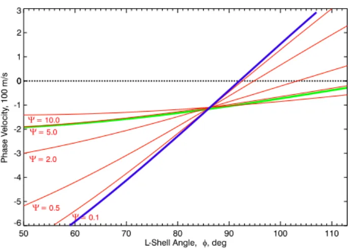
Y= 0.5 Y= 2.0 Y= 5.0 Y= 10.0
Y= 0.1
Fig. 6. Phase velocity versusL-shell angle. By the blue (green) line we show the fitted curve for F (E) region from Fig. 3. The predictions of the linear fluid theory calculated by assuming the ion drift Vi0 that is ten times smaller and rotated by 90◦ with
respect to the electron driftVe0 (which is estimated from the F-region velocity measurements, blue curve) and for anisotropy fac-tors9=0.1,0.5,2.0,5.0, and 10.0 are shown by the red curves.
depressed below it. The reason for this effect is not entirely clear, and we consider here two possibilities.
Makarevitch et al. (2002b) and Milan et al. (2003) pro-posed that low-velocity HF echoes are coming from the bot-tom of the unstable E-region, where the Doppler velocity is smaller because of increased collisions with neutrals. Let us comment on how this hypothesis helps in understanding the data presented in this study.
According to the linear fluid theory of electrojet irregu-larities (e.g. Fejer and Kelley, 1980), the phase velocity at a direction of wave propagation vectorkˆ≡k/ kis given by
V = ˆk·Ve0+9Vi0
1+9 , (1)
where the anisotropy factor 9 (Sahr and Fejer, 1996) is a function of aspect angleα, collision frequencies of ions and electrons with neutrals (νi,νe) and ion and electron
gyrofre-quencies (i, e):
9= νeνi
ei
(cos2α+
2
e
ν2
e
sin2α). (2)
The expressions for both electron and ion background drift velocity (Vα0, α=e, i) can be readily obtained from
the zeroth order momentum equations (e.g. Schlegel and St.-Maurice, 1981):
Vα0=
1 1+(να/ α)2
E×B
B2 +
να
α E
B
. (3)
In the E-region (say, below 120 km),νe≪e, νi≫i, and Ve0∼=
E×B
B2 , Vi0∼=
i
νi E
B, (4)
which means that the ion drift velocity is much smaller than that of electrons and rotated with respect to it by∼90◦.
We note that Eq. (1) predicts proportionality between the irregularity velocity and the electron plasma drift, since the first term dominates in a broad range of flow angles with the exception of observations close to the perpendicular-ity to Ve0. An increase in collision frequencies νe, νi
re-sults in the corresponding increase in the anisotropy fac-tor 9 and decrease in the irregularity phase velocity, be-cause of the 1+9 factor in the denominator. The calcu-lations based on the formulas for collision frequencies by Schunk and Walker (1973) and Schunk and Nagy (1978) give
νi∼1.5·104s−1,νe∼105s−1and hence, an anisotropy factor
of9(α=0)=νiνe/(ii)∼1 at an altitude of 95 km. Thus,
we can estimate that this purely collisional depression of the Doppler velocity in the lower E-region (below 95 km) can be as large as 2 times, which can partially explain our observa-tions.
However, this is still less than the reported factor 5. We think that another effect might be involved, namely the effect of echo reception from a range of altitudes with quite different aspect angles, as described recently by Uspensky et al. (2003). According to the model of Uspen-sky et al. (1994, 2003), auroral backscatter is always non-orthogonal since the purely non-orthogonal component, coming from just one height, constitutes only a fraction of all echo power. This means that observations at any spot of the iono-sphere can be characterized by some finite effective aspect angle. An increase in effective aspect angleαresults in the corresponding increase in the anisotropy factor9, Eq. (2), and decrease in the irregularity phase velocity. Estimates for the STARE radars showed that the effective aspect an-gle can be in the range of 0.8◦–1.0◦(Uspensky et al., 2003). If one adopts effective aspect angles comparable to the ones expected for STARE, one can explain additional velocity at-tenuation by a factor of 2–3.
Another consequence of the large anisotropy factor 9
is an increase in the ion motion Vi0 contribution to the
phase velocity and rotation of the direction of maximum phase velocity away from the electron flowVe0. The
lat-ter effect, reported by Uspensky et al. (2003) as the 10◦– 20◦azimuthal difference between F- and E-region velocity vectors seems to find some confirmation in the data of the present study. Indeed, Fig. 4 shows that while the F-region flow was more or less L-shell aligned (|φ0|<8◦), the
E-region flow was not, with the typical azimuthal difference between the flows larger than 15◦ (except of the last 30 min). Figure 6 shows the result of phase velocity calcu-lations based on Eqs. (1)–(3) for different anisotropy fac-tors 9 (red lines). For these calculations we assumed that the ion drift is ten times smaller and rotated by 90◦ clock-wise with respect to the electron drift, which is typical for the central part of the E-region (105–110 km),νi∼=1800 s−1
andVi0/Ve0=i/νi∼=1/10. The electron drift was estimated
agrees well with the fitted E-region velocity curve, suggest-ing that the anisotropy factor was indeed quite large. If so, one might wonder why exactly the anisotropy factor was so large. As we argued, the enhanced collision frequencies at the bottom of the E-region coupled with the effectively non-orthogonal scatter can be a reason, but in this scenario the ion drift would be too small (of the order of 1/100Ve0only)
to cause any significant shift in the E-region velocity rever-sal direction from 90◦of the flow angle (e.g. similar to those in Fig. 6). This is why in the reasoning above we assumed that the E-region echoes originated mainly from the electro-jet center.
An important new result of this study is that for large flow angle observations (φ>90◦), the E-region velocities were at minimum at a range r0 where the echo power was at
maximum and where the model aspect angle was around zero (Fig. 2c and right part of Fig. 3, where instead of V-structures,3-structures were observed). This velocity de-crease nearr0is very unlikely to be caused by the decrease
in the electric field intensity at these ranges, since the DMSP convection component is quite stable over this area, Fig. 1. To some extent, this result reminds us of observations of Makarevitch et al. (2002a), who reported the absence of the aspect angle attenuation for the Doppler velocity at large
L-shell anglesφ∼=90◦. Makarevitch et al. (2002a) explained their result in terms of the ion drift contribution to the irreg-ularity phase velocity at large flow angles. We believe that a similar explanation can be applied to the present observa-tions, as outlined below.
Equation (1) can be rewritten in terms of the flow angle [θ≡cos−1(k·Ve0/kVe0] as
V∼=cosθ+9i/νisinθ
1+9 Ve0, (5)
or
V∼=
cosθ−i/νisinθ
1+9 +i/νisinθ
Ve0. (6)
One should note here that Eq. (6) is more appropriate for discussion of the aspect angle effects, since only the first term is dependent upon9and hence, upon the aspect angleα.
The simplest formulation of the linear fluid theory that takes into account only the electron motions predicts that the velocity should change withθ as Ve0cosθ/(1+9)and fall
off to zero with the aspect angleαincrease. If the ion mo-tions are included into calculamo-tions, the situation changes. In this case the phase velocity at large flow and aspect angles will be determined mostly by the ion drift l-o-s component or the second term in Eq. (6), since the first term is reduced drastically because of the enhanced anisotropy factor9 at large aspect angles.
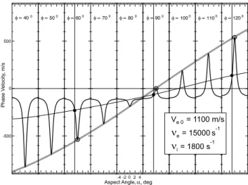
We illustrated this point in Fig. 7 which shows the results of the phase velocity calculations based on Eqs. (1)–(3). The phase velocity is shown in Fig. 7 as a function of the as-pect angle for various flow angles. As before, the typical (for the central part of the E-region) collision frequencies
νi=1800 s−1, νe=15 000 s−1 were assumed, as well as the
f= 400
-500 0 500
f= 500 f= 600 f= 700 f= 800
-4 -2 0 2 4 Aspect Angle,a,deg
f= 900 f= 1000 f= 1100 f= 1200
PhaseV
elocity
,m/s
V = 1100 m/s
= 15000 s
= 1800 s e 0
n n
e
i
-1
-1
Fig. 7.Phase velocity versus aspect angleαfor variousL-shell an-glesφassuming exactlyL-shell aligned electron flow (θ=φ)Ve0=
1100 m/s and collision frequencies typical for the center of electro-jet region. The large grey (black) circles show the phase velocity atα=0◦(α= −1◦). The grey thick (black thin) line represents the flow angle variation of the phase velocity for minimum achievable aspect angle of 0◦(−1◦).
exactL-shell aligned electron flow,Ve0=1100 m/s. For each
panel of Fig. 7, theL-shell angle is constant (we indicated this angle at the top, for example, φ=40◦ for the leftmost panel), while the aspect angle is changing from−5◦to +5◦. Thus, each panel models radar observations in one beam po-sition.
Let us first have a look at the left part of the diagram (φ=40◦−70◦). The phase velocity magnitude maximizes at zero aspect angle and decreases with the aspect angle in-crease. The velocity at zero aspect angle is approximately equal to the l-o-s component of the electron drift velocity, and we connected points with perfect aspect angle (shown by grey circles) with the grey thick line, which is essentially a simple “cosine law” curveVe0cosθ, similar to the fitted
F-region cosine curves in Figs. 3 and 6.
At large aspect angles, however, velocity is not zero but some finite value, which is determined by the second ion term in Eq. (6). For our observations, the latter can be easily estimated from Eq. (4); the electron drift is∼1100 m/s and hence, the ion Pedersen drift is∼110 m/s and directed north-ward (along the polenorth-ward electric field in the afternoon sec-tor) that is away from the radar, providing a negative offset of ∼110 m/s in the E-region velocity, consistent with our obser-vations. Importantly, the phase velocity calculations show that for certain flow angles (as for φ=90◦ in Fig. 7), the phase velocity is less in magnitude at perfect aspect angle than at larger ones. This is simply because at these direc-tions the ion modirec-tions become more significant at large as-pect angles than the electron motions. This effect can explain the reported minimum in the high-number beam velocities at ranges nearr0that correspond to the power maximum and to
One can also notice that although the velocity decrease with the aspect angle is seen in Fig. 7 forφ=90◦, the range of theL-shell angles with the3-structures in Fig. 3 is much wider and extends from φ∼=85◦ to 113◦. Another discrep-ancy between Figs. 3 and 7 is that the maximum Doppler velocities recorded were much smaller in magnitude than, for example,−500 m/s that should be observed nearφ=60◦. Following Uspensky et al. (2003), we argued that this reduc-tion can be related to the HF backscatter signal collecreduc-tion from the range of heights with the different finite aspect an-gles, which is equivalent to assigning some effective nonzero aspect angle to a specific range.
We can now estimate the effect of the aspect angle “finite-ness” on the flow angle dependence using the presentation of Fig. 7. We indicated by vertical lines the aspect angle of−1◦, by black dots the theoretical velocities which correspond to this aspect angle atφ=60◦, 90◦, and 120◦, and connected these points by the thin black line. The phase velocity is greatly reduced, especially for directions away fromφ=90◦. For example, forφ=60◦, it changes from∼500 to 200 m/s. Another interesting feature is that the black curve intersects the zero velocity line to the right from the grey curve, mean-ing that the phase velocity should be reversed at flow angles of more than 90◦, consistent with our measurements. On the other hand, in our observations the E-region velocity re-versal was not seen anywhere in the radar FoV, even at the easternmost beam 15 (φ∼110◦), while according to Fig. 7 this reversal should occur somewhere between 90◦and 110◦. One should note here, however, that in the reasoning above we used a minimum aspect angle of−1◦, consistent with an estimate for the STARE radar (144 MHz) obtained by Us-pensky et al. (2003), who adopted an aspect sensitivity of 10 dB per 1◦of aspect angle. Haldoupis (1989), by consider-ing the publications on the aspect sensitivity at various radar frequencies, concluded that the 50-MHz E-region echoes are perhaps less aspect sensitive than those at 150 and 400 MHz, with the typical values in the range 1–3 dB/◦. Thus, if one assumes a slower rate of the power decrease with the aspect angle for observations at lower HF frequencies, say, 2 dB/◦ reported recently by Makarevitch et al. (2002a), one can ar-gue that the effective aspect angle at HF should be larger and hence, one can reach better agreement between observations and theory.
On a more critical note, from Eq. (5) the flow angle cor-responding to a maximum of the phase velocity (or, in other words, the deviation of the flow from theE×Bdirection) is given by tanθmax=9i/νi and hence for fixed collision
fre-quencies/altitude should not depend upon the flow intensity
Ve0. Experimentally, Fig. 4 shows that this deviation tends
to decrease in magnitude with a drift magnitude decrease, suggesting that perhaps other (than Pedersen motion of ions) factors can contribute to the total ion drift vector, for exam-ple, the neutral wind. The detailed discussion of this issue is, however, beyond the scope of the present paper. We would like only to point out that even a simple ion Pedersen drift interpretation explains reasonably well most of the Doppler velocity features observed in this study (small magnitudes,
deviation from theE×Bdirection, and the spatial anticorre-lation with the backscatter power).
4 Summary and conclusion
A comparison of the F- and E-region HF Doppler velocities observed by the CUTLASS Finland radar shows that the E-region velocities are typically several times smaller and do not exhibit a change in their sign (within the radar FoV), as opposed to the F-region velocities. The E-region veloc-ity variation with L-shell angle φ can be described by a shifted cosine functionV0cos(φ+φ0), with the typical
val-ues ofV0= −200 m/s,φ0=−30◦. For the high-number radar
beams, the Doppler velocity is minimized at slant ranges that correspond to the power maxima and minimum aspect angle, as determined from the model. The observed difference be-tween F- and E-region HF Doppler velocities, as well as the velocity magnitude increase with the aspect angle atφ>90◦, cannot be explained by the electric field magnitude and direc-tion variadirec-tion with latitude, but most likely is a result of the non-orthogonality of backscatter coupled with the ion mo-tion contribumo-tion to the E-region irregularity phase velocity significant at large flow and aspect angles.
Acknowledgements. The CUTLASS radars are funded by PPARC, the Finnish Meteorological Institute, and the Swedish Institute for Space Physics. The IMAGE magnetometer data are collected as a Finnish-German-Norwegian-Polish-Russian-Swedish project. The IRIS riometer and the SAMNET magnetometers are funded by PPARC. We are very grateful to F. J. Rich of AFRL and V. O. Pa-pitashvili of University of Michigan for providing the DMSP drift-meter data. We would like to thank the ACE Science Center and N. F. Ness for providing the ACE magnetic field data. R. A. M. gratefully acknowledges funding from PPARC. This work was also supported by NSERC (Canada) grant to A. V. K.
Topical Editor M. Lester thanks S. Milan and another referee for their help in evaluating this paper.
References
Baker, K. B. and Wing, S.: A new magnetic coordinate system for conjugate studies at high latitudes, J. Geophys. Res., 94, 9139– 9143, 1989.
Bilitza, D.: International reference ionosphere 2000, Radio Sci., 36, 261–275, 2001.
Davies, J. A., Lester, M., Milan, S. E., and Yeoman, T. K.: A com-parison of velocity measurements from the CUTLASS Finland radar and the EISCAT UHF system, Ann. Geophysicae, 17, 892– 902, 1999.
Fejer, B. G. and Kelley, M. C.: Ionospheric irregularities, Rev. Geo-phys., 18, 401–454, 1980.
Foster, J. C. and Erickson, P. J.: Simultaneous measurements of E-region coherent backscatter and electric field amplitude at F-region heights with the Millstone Hill UHF radar, Geophys. Res. Lett., 27, 3177–3180, 2000.
H.: DARN/SuperDARN: A global view of the dynamics of high-latitude convection, Space Sci. Rev., 71, 761–796, 1995. Haldoupis, C.: A review on radio studies of auroral E-region
iono-spheric irregularities, Ann. Geophysicae, 7, 239–258, 1989. Koustov, A. V., Danskin, D. W., Uspensky, M. V., Ogawa, T.,
Jan-hunen, P., Nishitani, N., Nozawa, S., Lester, M., and Milan, S.: Velocities of auroral coherent echoes at 12 and 144 MHz, Ann. Geophysicae, 20, 1647–1661, 2002.
Makarevitch, R. A., Koustov, A. V., Sofko, G. J., Andre, D., and Ogawa, T.: Multifrequency measurements of HF Doppler velocity in the auroral E-region, J. Geophys. Res., 107(8), doi:10.1029/2001JA000268, 2002a.
Makarevitch, R. A., Koustov, A. V., Igarashi, K., Sato, N., Ogawa, T., Ohtaka, K., Yamagishi, H., and Yukimatu, A. S.: Comparison of flow angle variations of E-region echo characteristics at VHF and HF, Adv. Polar Upper Atmos. Res., 16, 59–83, 2002b. Milan, S. E. and Lester, M.: Simultaneous observations at
differ-ent altitudes of ionospheric backscatter in the eastward electrojet, Ann. Geophysicae, 16, 55–68, 1998.
Milan, S. E., Lester, M., and Sato, N.: Multi-frequency observations of E-region HF radar aurora, Ann. Geophysicae, 21, 761–777, 2003.
Nielsen, E. and Schlegel, K.: A first comparison of STARE and EISCAT electron drift velocity measurements, J. Geophys. Res., 88, 5745–5750, 1983.
Nielsen, E., and Schlegel, K.: Coherent radar doppler measure-ments and their relationship to the ionospheric electron drift ve-locity, J. Geophys. Res., 90, 3498–3504, 1985.
Nielsen, E., del Pozo, C. F., and Williams, P. J. S.: VHF coherent radar signals from the E-region ionosphere and the relationship to electron drift velocity and ion acoustic velocity, J. Geophys. Res., 107(1), doi:10.1029/2001JA900111, 2002.
Robinson, T. R.: Towards a self-consistent nonlinear theory of radar aurora backscatter, J. Atmos. Terr. Phys., 48, 417–422, 1986.
Robinson, T.: Simulation of convection flow estimation error in VHF bistatic auroral radar systems, J. Atmos. Terr. Phys., 11, 1033–1050, 1993.
Ruohoniemi, J. M., and Baker, K. B.: Large-scale imaging of high-latitude convection with super dual auroral radar network HF radar observations, J. Geophys. Res., 103, 20 797–20 811, 1998. Sahr, J. and Fejer, B. G.: Auroral electrojet plasma irregularity theory and experiment: A critical review of present understand-ing and future directions, J. Geophys. Res., 101, 26 893–26 909, 1996.
Schlegel, K.: Coherent backscatter from ionospheric E-region plasma irregularities, J. Atmos. Terr. Phys., 58, 933–941, 1996. Schlegel, K. and St.-Maurice, J.-P.: Anomalous heating of the polar
E-region by unstable plasma waves, 1. Observations, J. Geophys. Res., 86, 1447–1452, 1981.
Schunk, R. W. and Nagy, A. F.: Electron temperatures in the F-region of the ionosphere: Theory and observations, Rev. Geo-phys. Space Phys., 16, 355–399, 1978.
Schunk, R. W. and Walker, J. C. G.: Theoretical ion densities in the lower ionosphere, Planet. Space Sci., 21, 1875–1896, 1973. St.-Maurice, J.-P., Choudhary, R. K., Ecklund, W. L., and Tsunoda,
R. T.: Fast type-I waves in the equatorial electrojet: Evidence for nonisothermal ion-acoustic speeds in the lower E-region, J. Geophys. Res., 108(5), doi:10.1029/2002JA009648, 2003. Uspensky, M. V., Kustov, A. V., Sofko, G. J., Koehler, J. A., Villain,
J.-P., Hanuise, C., Ruohoniemi, J. M., and Williams, P. J. S.: Ionospheric refraction effects in slant range profiles of auroral HF coherent echoes, Radio Sci., 29, 503–517, 1994.