Article
Printed in Brazil - ©2016 Sociedade Brasileira de Química 0103 - 5053 $6.00+0.00
*e-mail: [email protected]
Estuary Adjacent to a Megalopolis as Potential Disrupter of Carbon and Nutrient
Budgets in the Coastal Ocean
Letícia Lazzari,*,a Angela L. R. Wagener,a Cássia O. Farias,b Aída P. Baêta,a Cristiane R.
Mauad,a Alexandre M. Fernandes,b Rodolfo Paranhosc and Renato S. Carreiraa
aDepartamento de Química, Pontifícia Universidade Católica do Rio de Janeiro,
22453-900 Rio de Janeiro-RJ, Brazil
bFaculdade de Oceanografia, Universidade do Estado do Rio de Janeiro,
20550-900 Rio de Janeiro-RJ, Brazil
cInstituto de Biologia, Universidade Federal do Rio de Janeiro,
21941-617 Rio de Janeiro-RJ, Brazil
The goals were to estimate nutrients and carbon flow rates between Guanabara Bay and the adjacent coastal waters, to characterize the provenance of the exported/imported organic matter. Samples were collected from different depths over 25 h in two seasons at the bay entrance. Measurements included physicochemical parameters, nutrients, chlorophylls, dissolved organic carbon (DOC), particulate organic carbon (POC), particulate nitrogen (PN), carbon (d13C) and nitrogen (d15N) isotopic composition, sterols in suspended particulate matter (SPM) and bacterioplankton. Most variables showed higher values in ebb tide events. The flow rates calculated on daily basis and estimated on annual basis revealed the exportation to the continental shelf of 1.27 × 10⁴ kmol year-1 dissolved inorganic nitrogen (DIN), 9.52 × 10² kmol year-1 dissolved inorganic phosphorus (DIP), 2.65 × 10⁴ t year-1 DOC, 1.96 × 10⁴ t year-1 POC, and 2.96 × 10⁴ t year-1 PN. The estimates show the bay contributes with 0.01% of the total global carbon influx to the ocean.
Keywords: organic carbon, nutrients, flow rates, sterols, carbon and nitrogen isotopes
Introduction
Coastal environments play an important role in the biogeochemical cycles and budgets of carbon and nutrients on a global scale.1 The changes of these cycles and budgets result in high rates of primary and secondary production, and also increase the flux and transformation rates of organic matter (OM) along the river/estuary/coastal-sea continuum.2-5
The cycle of OM in coastal systems, as in estuaries and bays, is highly dynamic and complex. In part, this results from the constant change in the relative contribution and distribution of OM from autochthonous and allochthonous sources, which is modulated by variations in freshwater regime and tidal forcing.6-9 Turbulent mixing of fresh- and sea-water can also generate sudden changes in temperature, salinity, turbidity, pH and bioactive element concentrations in time scale of seconds to months.7
Superimposed to the aforementioned natural factors, in many urbanized areas raw or only partially treated sewage is released directly into adjacent aquatic systems. The introduction of these nutrient rich effluents into water bodies with restricted water circulation can cause eutrophication.10,11 It is also the cause of less evident problems including high economic losses,11 changes in the ecological structure12 and decreased levels of dissolved oxygen (DO).13,14 In addition to alterations directly affecting the receiving body, the nutrient load may be transported to inner and mid shelf areas, in the dissolved and particulate forms, and thereby changing the carbon balance and fixation rates in the marine system.15 It has been considered, for instance, that nutrient and carbon exports originating from areas contaminated by sewage may be directly related to ocean acidification processes, and associated with climatic changes.1,15,16
addressed qualitative aspects, whereas a quantitative approach including, for instance, the influence of material transferred along the estuarine gradient is less frequently observed.21-23
Selman et al.24 provide strong evidences of the growing
global impact of eutrophication, identifying 415 eutrophic and hypoxic coastal systems around the globe, including the coastal region of Rio de Janeiro and other areas in the south-southeastern coast of Brazil.
The warm and nutrient poor waters of the Brazil current dominate a large portion of the Brazilian inner and mid shelf. In the mid shelf area off Rio de Janeiro, on the other hand, the upwelling of South Atlantic central waters (SACW) is a strong seasonal phenomenon that creates areas of enhanced primary production. Besides the fertilization by upwelling, the region receives nutrient and OM inputs from the eutrophic Guanabara Bay (GB), whose hydrographic basin houses nearly 12 × 106 inhabitants.25 GB is considered to be one of the most polluted coastal systems in Brazil, where the foremost contamination derives from untreated domestic effluents.26-28
The high eutrophication of GB results in enhanced local rates of primary production, reaching values of 0.17 mol C m-2 day-1.29 The annual input of 3.2 × 10¹⁰ mol P and 6.2 × 10¹⁰ mol N, mostly originated from untreated sewage discharge, has been estimated by Wagener.28 A fraction of the highly available nutrients and OM derives from industrial activities producing about 150 tons of effluents per day.27,30
In the present study, GB was taken as a model system to investigate the potential impact of highly eutrophic environments on the nutrient and carbon global balance in coastal zone and to estimate its relevance as a source of these materials to the inner continental shelf.
For this purpose, physicochemical and biogeochemical properties of the water column were studied over tidal cycles in the dry and wet seasons providing also information on the origin of particulate organic carbon (POC) through the use of elemental (C and N) and isotopic (d13C and d15N) composition. Sterols were also considered as additional indicators of the sources of OM in the studied region.
Experimental
Study area
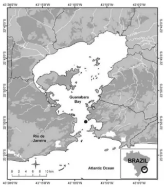
Guanabara Bay (Figure 1), one of the largest bays in the Brazilian coast, is circumscribed by the metropolitan area of Rio de Janeiro (22o40’-23o00’ S, 43o00’-43o20’ W) serving as estuary for more than 45 rivers and streams, of which only six are responsible for 85% of total annual freshwater discharge.
The surface area of the bay is approximately 384 km2 and the average volume of water is around 1.87 × 10⁹ m3. The average depths in the shallowest area are of 3 m, and in the central portions water depth ranges from 30 to 40 m.31-33
The influx of fresh water to GB is not sufficient to modify the flow pattern of the water in the bay because the ratio of fresh water runoff to tidal prism for a period of 24 h is less than 5%.33 However, riverine inputs are important for determining some patterns and water mass exchanges. The effects of riverine contribution on the receiving system depend on the use and occupation of the drainage basin. In systems adjacent to highly industrialized areas, such as GB, in addition to nutrient inputs, environmental conditions are significantly altered due to releases of trace metals, hydrocarbons, other potentially toxic substances and OM.33,34
The tidal influence is very important in the bay especially due to the intensity of the current velocities, which range from 80 to 150 cm s-1 at the bay mouth decreasing to 30-50 cm s-1 in the inner areas. The average tidal amplitude is of 0.7 m, varying from 1.1 m in spring tide to 0.3 m in neap tide.35 Salinity varies in the range of 29.5 ± 4.8 and reported average surface water temperature is 24.2 ± 2.6 oC.33
Sampling
A sampling station (Figure 1) was strategically positioned as to allow the observation of tidal influence and
exchange of materials between the bay and the open coastal area. Two sampling campaigns (the dry season sampling (C1) was in June 2011, and the wet season campaign (C2) occurred in November 2011) were performed, and the total monthly precipitation for C1 was 32.7 mm and for C2 it was 93.3 mm. Both samplings occurred in spring tide due to the higher amplitude variation (3.4 m for both) between low and high tides. Water samples were taken at each 2 h from three different depths: surface (S, < 1 m), mid-depth (M, 5 m) and close to the bottom (F, 25 m). Sampling was conducted aboard the parcel ship and the local depth varied from 28 to 30 m.
Salinity, temperature and depth were monitored through a conductive, temperature and depth (CTD) system (SBE, model 19 plus V2 SEACAT; frequency 4 Hz) to obtain a full water profile characterization. The data were processed on MatLab (R2008a) using only the data collected when the instrument was submerged and the average calculation for each 0.5 m of depth. The pressure inversions data were removed and also all the unrealistic values were removed based on the thermohaline index for the local water mass. The temperature and salinity data were filtered in order to remove peaks that exceeded values 3 times the standard deviation around the mean. An acoustic doppler current profiler (ADPC) WorkHorse 600 KHz was installed to obtain current data. Current components were corrected for magnetic decline and a small rotation of 22o W in relation to the geographic North. DO was measured with Alfakit AT 150 oximeter (range 0.01 to 20.00 mg L-1) and the pH was measured with Thermo Scientific Orion 3-Star (range –2 to 19.999), both in situ.
Water samples for organic compounds (sterols), elemental and isotopic compositions (C and N) of the suspended particulate matter were collected at each depth by using an amber glass bottle that was inserted closed into the water column. Bottles containing samples were kept under ice until filtration in the lab. For nutrients and chlorophyll determinations 4L Go-Flo bottles were used for sampling and samples were stored in 1.5 L polyethylene bottles under refrigeration. Samples for bacterioplankton counting (Bact) were stabilized with p-formaldehyde
immediately after sampling and thereafter kept in liquid N2. Samples for ammonium (NH4+) determination were stored in 50 mL glass tubes with screw cap after fixation
in situ as described in Grasshoff et al.36
For separation of the particulate matter samples were filtered in the lab. Those intended for sterol determination were filtered in Macherey-Nagel 142 mm diameter, 0.7 µm porosity glass filters. Samples for POC, particulate nitrogen (PN), d13C and d15N were filtered in Macherey-Nagel 47 mm, 0.7 µm glass filters. For chlorophyll determination,
filtration through cellulose acetate filters was applied before filter immersion in 90% acetone-water solution following Parsons.37 The filtrate was stored at –20 oC in polyethylene bottles for dissolved inorganic nutrient analyses.
Analytical procedures
Nutrients (nitrate (NO3–), nitrite (NO2–), ammonium (NH4+), inorganic dissolved phosphorus (Pinorg)) were determined following the methods described by Grasshoff et al.36 Chlorophylls (Chl-a, Chl-b and Chl-c)
were determined using the method of Parsons37 and equations given by Jeffrey and Humphrey.38 A DMS 100 UV-Vis spectrophotometer (Intralab, PerkinElmer) was used and all variables were determined in duplicate. The analytical variability was < 2%. Quality control included calibration curves with r > 0.99. Blanks were treated as samples for zero calibration in the spectrophotometer. Limits of detection (LOD) for nutrient determinations were the lowest concentration detected with precision 0.01 µmol L-1 for NO
3– and NO2–; 0.1 µmol L-1 for NH4+; and 0.02 µmol L-1 for Pinorg. Bact was analyzed by flow cytometry.39,40
Dissolved organic carbon (DOC) was determined in a Shimadzu total organic carbon (TOC)-VCPN analyzer (samples determined in duplicate). The LOD was equal to 3 × standard deviation (SD) of 10 blanks / slope of the calibration curve = 0.35 mg L-1 and limit of quantification (LOQ) = 3.33 × LOD was 1.15 mg L-1.
d13C and d15N of the particulate organic matter was determined in a Thermo Scientific Flash EA 1112 Delta V Plus isotope-ratio mass spectrometer (IRMS). For reference gases calibration and determination of LOD and LOQ the standard reference material U. S. Geological Survey (USGS) 40 (L-glutamic acid) purchased
from the International Atomic Energy Agency (IAEA) (–26.389 ± 0.042‰ Vienna Pee Dee Belemnite (VPDB) for d13C and –4.5 ± 0.1‰ air N
2 for d15N) was used. Reported values are the mean of triplicate determinations and those considered as valid measurements were generating pulses > 500 mV for carbon and > 800 mV for nitrogen.
Extraction of sterols was based on the U. S. Environmental Protection Agency (EPA) 3540C method.41 Filters containing the suspended particulate matter (SPM) were freeze dried and weighed before addition of the surrogate standard (5α-androstan-3β-ol) and Soxhlet extracted with 250 mL of dichloromethane over 24 h. Following extract concentration in a rotary evaporator, solvent was exchanged to hexane before fractionation in a glass column (7 g alumina, 2% deactivated silica gel and 1 g Na2SO4) to isolate aliphatic (F1) and aromatic hydrocarbons (F2) not considered in the present work. Only the fraction of interest, containing the sterols (F3), was then cleaned up using dichloromethane:methanol (9:1). To F3, evaporated to dryness under N2 flow, 250 µL of acetonitrile and 100 µL of bis(trimethylsilyl)trifluoroacetamide (BSTFA) were added for derivatization under 80 oC for 1 h. Lastly, the extracts were dried and the final volume adjusted to 1 mL with dichloromethane after addition of cholestane (2500 ng) as internal standard.
Sterols were determined in a Finnigan Focus DSQ gas chromatography-mass spectrometry (GC-MS) system operated in the electron ionization (EI, 70 eV) and full scan (m/z 50-550) modes. A DB-5 type column (5%
methyl-phenyl siloxane, 30 m × 0.32 mm × 0.25 µm film) was used. Quantification in the GC-MS was performed using a calibration curve (100 to 5,000 ng mL-1) with commercial standards [cholest-5-en-3β-ol (27∆5), 5α -22-cholestan-3β-ol (27∆0), 24-methylcholest-5-en-3β-ol (28∆5), 24-ethylcholesta-5,22-dien-3β-ol (29∆5,22) and 24-ethylcholest-5-en-3β-ol (29∆5)] and considering the peak areas of key ions (m/z 129 and 215 for unsaturated
and saturated sterols, respectively; m/z 370 for coprostanol
(5β-cholestan-3β-ol) and m/z 368, 394 or 396 for sterols
with double bond in C22). Similar response factors for key ions were assumed for structurally related compounds for which standards were not commercially available. GC-MS compound assignments were based on the full scan mass spectra obtained from the available standards (see above) or by comparison with mass spectra found in the literature
for the other compounds. Cholestane (5α-cholestane,
m/z 217) was used as quantification internal standard
and androstanol (5α-androstan-3β-ol) was the surrogate standard quantified by the m/z 333. LOD (LOD = 3 × SD
of 10 blanks / slope of the calibration curve) and LOQ (first point of the calibration curve > 3.33 × LOD) were 0.01 and 100 ng mL-1, respectively.
Statistical data evaluation
The software Statistica 11 was used for data evaluation through Pearson correlation test, Kruskal-Wallis test, and principal component analysis. Further information is given in Results and Discussion. All discussions referring to differences or similarities are based on the results of the statistical analysis using p < 0.05 for decision.
Results and Discussion
Characterization of the water column and physicochemical properties
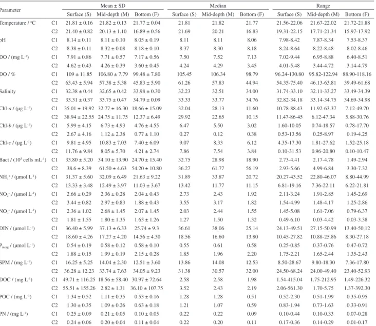
The average values, standard deviations and range for all physicochemical and geochemical parameters are given in Table 1.
The temperature (T) and salinity (Sa) diagram revealed distinct water column stratification especially in C2 (Figure 2).
In C1, temperatures were around 22 oC at all depths and the salinity varied slightly in the range of 32 to 34.5, with lower values in the surface. These values indicate that coastal waters, which are characterized by Sa < 33, dominated most samples collected in C1 at all depths. In C2, there was a linear correlation between T and S, marked by predominance of cold (T < 18 oC) and saline waters (Sa > 34.5) at the bottom and in mid-depth. These properties indicate the influence of SACW identified in the bottom by temperatures below 20 oC and salinities in the range of 34.6 to 36.2.42 The plot of salinity against temperature for C1 and C2 can be seen in Supplementary Information Figure S1. The current intensity and direction is shown in Figure 3.
The pH values were higher in the surface due to interaction between respiration, production and water-atmosphere exchange processes. The consumption of CO2 by photosynthesis causes an increase in pH, while the production of CO2 during respiration leads to a decrease in pH. In general pH was more elevated in C2 (p < 0.05),
Table 1. Means, standard deviations (SD), medians and ranges for all physicochemical and geochemical parameters in surface, mid-depth, and bottom layers in C1 and C2
Parameter Mean ± SD Median Range
Surface (S) Mid-depth (M) Bottom (F) Surface (S) Mid-depth (M) Bottom (F) Surface (S) Mid-depth (M) Bottom (F) Temperature / oC C1 21.81 ± 0.16 21.82 ± 0.13 21.77 ± 0.04 21.81 21.82 21.77 21.56-22.06 21.67-22.02 21.72-21.88
C2 21.40 ± 0.82 20.13 ± 1.10 16.89 ± 0.56 21.69 20.21 16.83 19.31-22.15 17.71-21.34 15.97-17.92
pH C1 8.14 ± 0.11 8.11 ± 0.10 8.05 ± 0.19 8.11 8.11 8.06 7.98-8.42 7.87-8.34 7.53-8.37
C2 8.38 ± 0.11 8.32 ± 0.08 8.18 ± 0.10 8.37 8.30 8.18 8.24-8.64 8.22-8.48 8.02-8.46
DO / (mg L-1) C1 7.91 ± 0.86 7.71 ± 0.57 7.17 ± 0.56 7.50 7.52 7.13 7.02-9.44 6.95-8.88 6.40-8.51
C2 4.62 ± 0.43 4.26 ± 0.39 3.60 ± 0.45 4.24 4.29 3.45 4.01-5.48 3.44-4.72 3.14-4.79
DO / % C1 109 ± 11.85 106.80 ± 7.79 99.48 ± 7.80 105.45 106.34 98.79 96.24-130.80 95.82-122.94 88.90-118.16 C2 63.43 ± 5.94 57.38 ± 5.38 45.83 ± 5.90 61.26 57.83 44.94 54.35-75.40 46.13-63.81 39.49-61.68 Salinity C1 32.38 ± 0.44 32.65 ± 0.42 33.98 ± 0.30 32.23 32.51 34.00 31.74-33.10 32.11-33.27 33.49-34.39 C2 33.31 ± 0.37 33.75 ± 0.47 34.79 ± 0.09 33.33 33.77 34.76 32.82-34.18 33.14-34.75 34.69-34.98 Chl-a / (µg L-1) C1 35.01 ± 19.92 32.77 ± 16.30 18.66 ± 15.09 32.04 28.13 11.60 10.78-88.43 11.92-63.37 7.12-49.70
C2 38.94 ± 22.55 24.75 ± 11.75 12.37 ± 6.49 29.92 22.65 10.15 11.47-86-45 6.12-47.34 5.88-30.76 Chl-b / (µg L-1) C1 5.99 ± 4.15 6.73 ± 4.93 4.76 ± 4.55 6.47 5.50 3.02 1.60-10.05 0.74-18.57 0.78-17.70
C2 2.67 ± 4.16 1.12 ± 2.38 0.77 ± 1.10 0.27 0.12 0.38 0.53-13.56 0.25-8.97 0.19-4.25
Chl-c / (µg L-1) C1 9.81 ± 4.95 10.83 ± 7.03 7.40 ± 6.09 9.07 8.33 6.12 4.35-17.30 1.81-27.62 1.52-25.18
C2 11.76 ± 9.84 8.05 ± 5.70 4.21 ± 2.74 7.86 7.54 3.84 0.10-31.53 0.96-20.80 0.10-10.47
Bact / (105 cells mL-1) C1 33.80 ± 5.20 34.10 ± 13.90 24.70 ± 15.40 32.75 28.98 18.90 2.73-4.41 2.17-4.78 1.49-2.94
C2 38.6 ± 8.39 61.50 ± 4.63 54.20 ± 10.80 36.27 61.77 56.19 2.93-5.66 4.99-6.84 3.30-7.32 NH4+ / (µmol L-1) C1 31.37 ± 5.60 32.09 ± 6.49 21.63 ± 9.22 31.89 33.87 20.72 20.27-43.52 22.80-46.07 8.80-44.99
C2 13.33 ± 3.48 12.49 ± 3.97 11.03 ± 3.67 13.42 11.77 11.15 6.81-19.16 7.36-22.11 6.22-21.81 NO2– / (µmol L-1) C1 2.66 ± 0.29 2.36 ± 0.28 2.04 ± 0.43 2.73 2.43 1.92 2.11-3.24 1.91-2.85 1.45-2.69
C2 3.44 ± 0.82 2.97 ± 0.83 1.88 ± 0.43 3.55 3.17 1.82 1.54-4.99 1.48-4.17 1.25-2.86
NO3– / (µmol L-1) C1 2.36 ± 1.02 2.68 ± 1.45 2.07 ± 1.45 2.03 2.44 1.55 1.45-5.08 1.61-7.06 0.79-6.37
C2 1.81 ± 1.55 1.80 ± 1.35 1.63 ± 1.26 1.27 1.50 1.32 0.49-6.10 0.03-4.42 0.03-3.38
DIN / (µmol L-1) C1 36.40 ± 5.99 37.13 ± 6.33 25.74 ± 9.3 36.61 38.06 25.14 24.13-49.51 27.15-50.99 13.40-50.12
C2 18.60 ± 4.26 17.27 ± 4.20 14.56 ± 4.30 18.56 16.60 13.80 10.45-27.82 10.88-25.86 8.30-27.18 Pinorg / (µmol L-1) C1 0.54 ± 0.19 0.58 ± 0.12 0.58 ± 0.10 0.55 0.61 0.58 0.25-0.85 0.37-0.76 0.47-0.72
C2 1.88 ± 0.15 1.99 ± 0.19 2.15 ± 0.28 1.85 1.96 2.20 1.75-2.21 1.65-2.44 1.35-2.43
SPM / (mg L-1) C1 16.25 ± 5.25 14.04 ± 2.30 12.51 ± 3.60 13.86 14.08 12.53 8.50-28.67 9.80-18.30 7.36-17.80
C2 36.28 ± 12.23 33.74 ± 7.63 34.05 ± 9.23 31.38 30.57 32.00 24.50-68.24 24.00-49.40 23.40-52.93 DOC / (mg L-1) C1 49.71 ± 116.25 18.56 ± 58.40 30.97 ± 72.64 2.58 2.58 1.98 1.54-415.04 1.75-212.95 1.49-226.32
C2 55.51 ± 155.26 2.82 ± 1.31 36.10 ± 107.75 3.52 2.43 2.19 2.06-561.30 1.70-5.75 1.37-392.30
POC / (mg L-1) C1 1.34 ± 0.52 1.11 ± 0.35 0.53 ± 0.16 1.28 1.28 0.51 0.52-2.30 0.51-1.99 0.35-0.95
C2 1.30 ± 0.35 1.09 ± 0.26 0.63 ± 0.18 1.21 1.07 0.59 0.83-1.94 0.73-1.63 0.33-0.91
PN / (mg L-1) C1 0.25 ± 0.09 0.21 ± 0.05 0.10 ± 0.05 0.22 0.22 0.09 0.10-0.44 0.10-0.33 0.07-0.28
C2 0.24 ± 0.06 0.20 ± 0.04 0.11 ± 0.04 0.22 0.20 0.11 0.17-0.36 0.14-0.29 0.01-0.17
SD: standard deviation; C1: dry season campaign; C2: wet season campaign; DO: dissolved oxygen; Chl-a, Chl-b, Chl-c: chlorophylls a, b and c; Bact: bacterioplankton; DIN: dissolved inorganic nitrogen; Pinorg: inorganic phosphorus; SPM: suspended particulate matter; DOC: dissolved organic carbon; POC: particulate organic carbon; PN: particulate
nitrogen.
Chl-a (r = 0.635; p < 0.01), of DO and bacteria counting
(r = 0.550; p < 0.01), as well as of Chl-a and bacteria
counting (r = 0.423; p < 0.01) only in C2 may be taken as an
indication of respiration activity (bacteria and other grazing) exceeding primary production in the entire water column including the photic zone.44 This may occur subsequent to the incidence of an algae bloom. Algae blooms have been frequently observed in the outer bay region as well as in the adjacent coastal region.44 DO and pH are correlated in the linear data fits (C1: DO = –17.98 + 3.15 pH, r = 0.603,
p < 0.05; C2: DO = –27.21 + 3.78 pH, r = 0.807, p < 0.05)
demonstrating dominance of biochemical process45 as
124%; bottom: 73%) to those found in C1. The lower DO levels in C2 compared to the 13 years average reveal occasions of eutrophic conditions aggravation in the outer region of the bay specially during the wet period.
The intensification of eutrophic conditions in areas of the bay with higher circulation is confirmed by the nutrient concentrations which were up to three times higher than those reported previously for the same area.33,47 This should be expected due to the combined effect of a submarine outfall installation in 2003 downstream of the sampling station and the population growth in recent years.25 NH
4+ was the most abundant nitrogen species, which showed strong seasonal variations with higher concentrations in C1
(p < 0.05). In both samplings concentrations of ammonium
were more elevated at mid-depth during ebb tide proving that OM degradation in the water column just below the euphotic zone is very intense as observed by Wagener28 and that the inner areas of the bay are important source of NH4+ derived from sewage release. Nitrite showed low seasonal variation being more elevated in surface waters in C2, while for C1 higher nitrate concentration occurred during flood tide (Figure 4) and higher concentration of NH4+ occurred in the ebb tide (Figure 4). Higher nitrate concentrations (3.7 µmol L-1) were reported in the past by Rebello et al.29 for surface waters and by Kjerfve et al.33for bottom waters (average for 13 years: 4.5 ± 3.4 µmol L-1). Such change is an additional indicator of a tendency towards further decay of the system with increasing NH4+.
Pinorg predominated in C2 especially at the bottom and variations in both samplings occurred without tide dependence. Higher concentrations in C2 bottom waters reveal the input from the SACW but a contribution from the sediments cannot be discarded in both C1 and C2.33,48
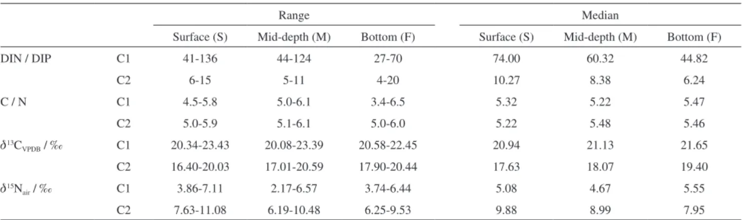
The ratio dissolved inorganic nitrogen (DIN) / dissolved inorganic phosphorus (DIP) was calculated considering all DIN species and the results are given in Table 2. By using the Redfield ratio N / P (16:1) it is possible to estimate that P is the limiting nutrient in C1 and also that the remobilization of P from sediments is substantial as the sharp DIN / DIP decrease from surface to bottom waters, especially in C1, and the trend to higher concentrations in the bottom suggest. In C2 N / P values were often below 16 indicating a strong relative P consumption.49
SPM was higher in C2 (p < 0.05) (see Table 1) possibly
due to the intense continental runoff during the rainy season. Kalas et al.50found in the sampling region values for SPM
in the range reported here.
The intense primary production in the bay is represented by the high Chl-a concentrations during the samplings,
with concentrations reaching more than 80 µg L-1 (Table 1). According to the Organisation for Economic Cooperation and Development (OECD),51 Chl-a concentrations above 25 µg L-1 are typical of eutrophic systems. The presence of higher values in C1 may be ascribed to the lower SPM found in the dry season since, as observed by Rebello et al.,29 primary production in the bay is limited by the water transparency. Chl-c is also a significant component of the
photosynthesized pigments and such observation concurs with the reported abundance of dinoflagellates in the bay.52,53
Heterotrophic bacteria are important for the structure and dynamics of food chains, as well as for the biogeochemical cycles, being responsible for the inter-conversion of DOC and POC in the carbon cycle.54 Bacterioplankton Figure 2. CTD full water profile characterization in C1 and C2 samplings.
CW: Coastal water; SACW: South Atlantic central waters.
abundance was similar in C1 and C2 as indicated by the Kruskal-Wallis test (Table 1) although variations with tide were very intense as indicative of the heterogeneity of the system. Maximum abundance was present at mid-depth, below the photic zone, as expected due to the fast recycling of organic matter typically occurring in the bay down in the water column.55 In C2 bacterioplankton abundance was
significantly correlated to NH4+ (r = 0.764, p = 0.001) and to POC (r = 0.500, p = 0.001). A low correlation is observed
with respect to d13C (r = 0.398, p = 0.01, s = 1.83). These associations during periods of water stratification when vertical transport is hindered as in C2 prove the intensity of bacterial activity at mid-depth resulting in residual organic material enriched in 13C and liberation of NH
4+. Figure 4. NO3– and NH4+ variation during 25 h tide in C1 and C2.
Table 2. Ranges and medians for DIN / DIP ratio, C / N ratio, d13C
VPDB (‰) and d15Nair (‰) at the surface, mid-water and bottom in C1 and C2
Range Median
Surface (S) Mid-depth (M) Bottom (F) Surface (S) Mid-depth (M) Bottom (F)
DIN / DIP C1 41-136 44-124 27-70 74.00 60.32 44.82
C2 6-15 5-11 4-20 10.27 8.38 6.24
C / N C1 4.5-5.8 5.0-6.1 3.4-6.5 5.32 5.22 5.47
C2 5.0-5.9 5.1-6.1 5.0-6.0 5.22 5.48 5.46
d13C
VPDB / ‰ C1 20.34-23.43 20.08-23.39 20.58-22.45 20.94 21.13 21.65
C2 16.40-20.03 17.01-20.59 17.90-20.44 17.63 18.07 19.40
d15N
air / ‰ C1 3.86-7.11 2.17-6.57 3.74-6.44 5.08 4.67 5.55
C2 7.63-11.08 6.19-10.48 6.25-9.53 9.88 8.99 7.95
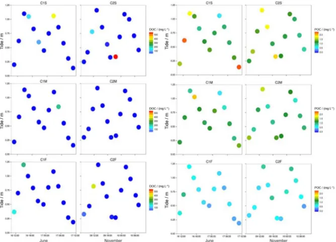
DOC was on average higher at the surface. The very elevated concentrations sporadically present (up to 400 mg C L-1) demonstrate the time variability of the system due to the influence of diffuse sources of sewage around the bay and to the sewage outfall located downstream of the sampling site (Figure 5).
Guenther et al.44 reports DOC values for the outer bay
area similar to those found in the present work except for the extremely high concentrations (overall DOC average and standard deviation after removing the extremes: 2.19 ± 0.48 mg L-1, n = 34 out of 39 samples in C1; 2.39 ± 0.68 mg L-1, n = 31 out of 39 samples in C2). Also, similar values are reported for the Pearl River in China.56 In polluted European estuaries, as the Sheldt estuary in Belgium and the Thames estuary in England, average concentrations are in the range of 5.8 to 6.8 mg C L-1 while in less altered estuaries, such as those of Gironde in France and of Douro in Portugal, DOC concentrations are from 2.5 to 3.1 mg C L-1.57
The data for Guanabara Bay fits well in the latter range in spite of being highly polluted. This can be understood on the basis of the fast degradation of organic matter under high temperatures and microbial activity, and the intensity of water exchange. According to Kjerfve et al.33the time for renewal
of 50% of the water volume (ca. 109 m3) in Guanabara Bay is only 11.4 days and this would explain the better water conditions in the most water-circulated areas, such as those near the bay mouth where the sampling point is located.
POC was more elevated at the surface during daytime in both samplings but in C1 the variations with depth were more prominent (Figure 5). The overall average POC concentration was of 1.00 ± 0.50 mg L-1 in C1 and 1.01 ± 0.39 mg L-1 in C2. In both samplings, DOC correlates significantly with POC if extreme DOC values are removed. The linear correlation parameters in C1 are: s = 0.41, r = 0.680, p < 0.05; in C2: s = 0.79, r = 0.715, p < 0.05.
POC and PN are very strongly correlated even if the entire data collection is considered (r = 0.997; p < 0.05). A
linear slope of 5.1 indicates predominance of autochthone organic matter in both campaigns.50 The C / N ratio of 4.4 (range 3.4 to 6.2; Table 2) indicates marine phytoplankton (C / N between 4 and 10)51 and bacterioplankton (C / N ca. 5) predominance.58,59
Carbon and nitrogen stable isotopes
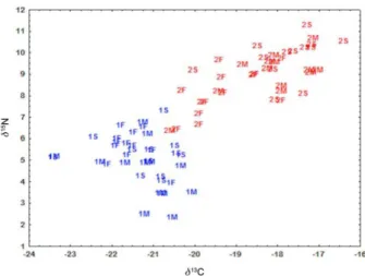
The plot of d13C vs.d15N (Figure 6) highlights the different properties of the system in the two samplings
and the significant linear correlation between the two isotopic ratios. C1 shows lower values for both d13C and d15N predominantly in the range of phytoplankton origin, however, the terrestrial influence was greater than in C2. C2 shows high values for both d13C and d15N indicating marine influence.
SPM, d13C and d15N also demonstrated a strong phytoplankton contribution to the organic matter pool (Table 2). In C1 the average for d13C was –21.35 ± 1.75‰ with only two values appearing below –23‰. These isotopic shifts are typically reported for autochthone OM (–19 to –25‰), according to Meyers.60 The presence of sewage-derived organic carbon, whose d13C is approximately –24‰,34 cannot be discarded; however, as observed by Carreira and Wagener,61 under the high regional temperatures the turnover rate of sewage OM and release of nutrients occur largely before reaching the marine environment. Kalas et al.50 reported d13C of
–21.30 to –15.10‰ for particulate organic matter in GB, similarly to the range found here in C1. In C2, the average for d13C shifted to –18.41 ± 1.11‰ and OM enriched in 13C (d13C = –16.40‰) was present. Such enrichment may
result from fast fixation rates and utilization of enriched dissolved inorganic carbon (DIC) produced during intense phytoplankton activity. Cifuentes et al.62 reported for periods of elevated primary production and during algae blooms carbon isotopic shift in the range of –18 to –12‰. The presence of POC enriched in 13C and other indications of phytoplankton predominance in C2 suggest utilization of dissolved carbon enriched in 13C and seem to reinforce the possible occurrence of an algae bloom just prior to the sampling. The significant correlation between the POC, made up mainly of autochthonous OM, and d13C (r = 0.632;
p < 0.05, s = 1.80) only in C2 may also be considered an
indication of 13C enrichment and primary fixation rates association.
C1 and C2 average values for d15N were 4.92 ± 1.13 and 8.79 ± 1.20‰, reaching a maximum of 7.11 and 11.08‰, respectively. In the marine environment, the predominant nitrogen incorporation mechanism includes nitrate reduction that generates nitrogen isotopic shifts between –2 and 4‰.63 According to Fogel and Cifuentes,64 d15N between 7 and 11‰ occurs principally when nitrate is the limiting nutrient, since in periods of elevated primary production phytoplankton consumes the available nitrate leading to enrichment in the heavier nitrogen isotope in the dissolved form.65 In coastal areas the contribution of dissolved nitrogen derived from anthropogenic activities (d15N of 7 to 30‰) has strong influence on the d15N of the SPM. Also, sediment trap studies have shown that microbial degradation of phytoplankton leads to increase in 15N in the residual OM.66,67 The 15N enriched OM in C2, as compared to C1, may result from the algae bloom occurring before the sampling day. The lower nitrate concentration and OM d15N close to 9-10‰ in C2 surface waters may derive, in addition, from nitrate consumption by dinoflagellates, the presence of which is confirmed by elevated Chl-c
concentrations. Low values of d15N in the range of –3 to 1‰, typical of N2 fixation,64 were not observed here. This is expected due to the abundance of dissolved nitrogen species in both samplings.
A factor analysis (FA) with varimax rotation was carried out with and without data normalization. As described in Massone et al.,68 the standard normalization is intrinsic to principal components analysis (PCA) as long as it is based on correlation matrix. The variables were grouped in four factors totalizing of 73% of variance. Salinity and temperature were very distinct in the two samplings and therefore were not used in the FA to avoid obscuring the differentiation of chemical properties. In the first factor (F1, 32% of the variance) are all variables that discriminate the two samplings: Pinorg, DO, SPM, d13C, d15N, NH4+ and pH. Samples with higher concentration of Pinorg, SPM, d13C, d15N and pH were positively correlated in F1, while those negatively correlated in F1 showed lower values of DO and NH4+. In the second factor (F2, 21% of variance) PN and POC are strongly correlated, which separates the samples according to the sampling depth. A third factor (F3, 12% of variance) includes DOC and POC and distinguishes the few samples appearing with unusually high concentration. The three chlorophylls are strongly correlated in F4 (8% of variance) and were not efficient in separating groups of samples, possibly due to the influence of depth and tidal variations. Figure 7 shows the graphical representation for the cases.
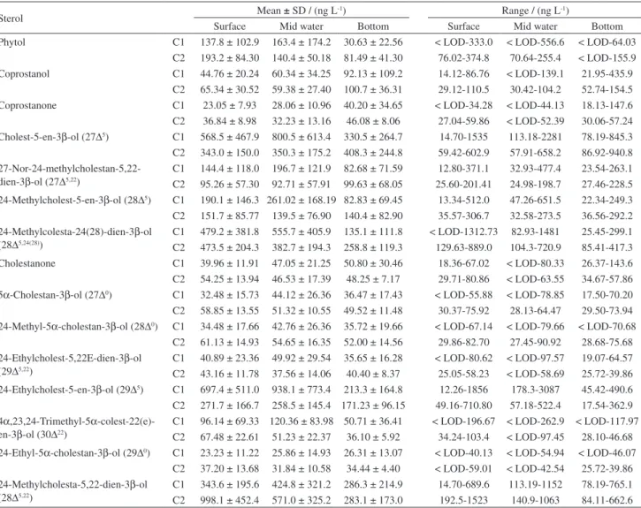
Sterols
Table 3 shows the results obtained for phytol and 15 sterols identified in the SPM. The average concentration of total sterols for C1 was 2,728 ± 2,058 ng L-1, which was slightly higher than the average value measured in C2, of 2,381 ± 1,006 ng L-1. Only 4 out of the 15 identified compounds made up the majority of the total sterols found in the present study. Cholest-5-en-3β-ol (cholesterol or 27∆5) was one of the most abundant sterols, representing, on average, 20.8 ± 24.2 and 15.5 ± 18.8% of the total sterols in C1 and C2, respectively. There was no clear evidence of 27∆5 concentration gradient with depth: the highest average value was at the mid-depth in C1 (800.5 ± 613.4 ng L-1) and in bottom water in C2 (408.3 ± 244.9 ng L-1). 27∆5 has been usually observed in natural waters at high concentrations due to its widespread occurrence in planktonic organisms and other animals.69 It is also found in raw sewage,70 and thus in contaminated coastal waters, such as in GB,26 the input of domestic effluents can be a relevant additional source of this sterol.
The sterol 24-methylcholesta-5,22-dien-3β-ol (28∆5,22) was also abundant, averaging 12.8 ± 12.2% of the total sterols in C1 and up to 26.3 ± 44.2% in C2. In fact, in C2 the 28∆5,22 exhibited the highest concentration amongst all sterols, with 998.2 ± 452.4 ng L-1 at the surface, 571.0 ± 325.2 ng L-1 at mid-depth and 283.16 ± 173.01 ng L-1 at the bottom. 28∆5,22 is produced by diatoms, dinoflagellates and prymnesiophytes.69-72 Another sterol associated with diatoms, such as Thalassiosira and Skeletonema,73,74 is 24-methylcolesta-24(28)-dien-3β-ol (28∆5,24(28)). In the present study, 28∆5,24(28) accounted for 14.4 ± 17.9% of the total sterols in C1, similarly to 28∆5,22; however, in the second sampling, 28∆5,24(28) accounted only for 9.9 ± 14.3% of the total sterol; it is a lower contribution as compared to 28∆5,22.
Another important sterol was 24-ethylcholest-5-en-3β -ol (29∆5), which represented 22.6 ± 29.7 and 9.9 ± 14.3% of the total sterols in C1 and C2, respectively. This sterol is generally considered typical of vascular (generally land) plants but is also present in some species of microalgae (prymnesiophytes) and it is possibly produced by cyanobacteria.50,69,70,75,76
Other phytosterols, such as 24-methylcholest-5-en-3β -ol (28D5) and 27-nor-24-methylcholestan-5,22-dien-3β-ol (27D5,22), accounted on the average for 5-6% of the total sterols. On the other hand, 4α,23,24-trimethyl-5α -colest-22(e)-en-3β-ol (30D22) made a remarkably low contribution (3.3 ± 3.4 and 22 ± 2.2% in C1 and C2, respectively) to the total sterols. 30∆22 is considered a consistent marker for dinoflagellates, although can also be found in some species of diatoms.77,78 Kalas et al.50reported the absence of 30∆22 in the SPM at the entrance of Guanabara Bay. Such feature is consistent with the occurrence of dinoflagellates especially in the northern part of the bay.79
The saturated sterols 5α-cholestan-3β-ol (27D0), 24-methyl-5α-cholestan-3β-ol (28D0) and 24-ethyl-5α -cholestan-3β-ol (29D0) were on the average below 2% of the total sterols in both samplings. The fecal sterol coprostanol contributed with 2.4 ± 3.3 and 3.1 ± 3.5% of the total sterols in C1 and C2, respectively. Similar values were also found for coprostanone, a fecal ketone.
Sterols as source assignments of OM
Sterols and phytol were used as a complimentary tool, in addition to bulk properties and isotopic composition of POC (as previously discussed), for source assignments of OM in the studied site. As these compounds have multiple and, in some cases, non-specific sources80 the sources assignment of OM using sterols was attained after a specific FA. The factor analysis applied to the entire sterol data set after normalization was not efficient in discriminating sampling campaigns and samples. Normalized data from C1 and C2 were then analyzed separately.
In both samplings, two factors accounted for 65-67% of the total variance (Figure 8). In Figure 8, the bi-dimensional plot of factor loadings (i.e., variables) shows similar groups of sterols (with some exceptions). For example, the major phytosterols discussed above (27∆5, 28∆5,22, 28∆5,24(28) and 29∆5) appear negatively correlated in factor 1 in C1 (except 28∆5,22) whereas in C2 they are positively correlated in this factor. Similar pattern was observed for coprostanol and for other less abundant sterols.
It is interesting to note in Figure 8 that in spite of 27∆5 being positioned distant from the other most abundant phytosterols, it appears always correlated with 27∆5,22 and Figure 7. Factor analysis including Pinorg, DO, SPM, d13C, d15N, NH4+,
28∆5. Such grouping is not easy to explain; it might well reveal the occurrence of grazing, as 27∆5 is more abundant in zooplankton and/or fecal pellets.79 Anyway, there are few samples (scores represented in Figures 8c and 8d) associated with this group. The grouping of 29∆5 with the phytosterols in both samplings suggest an autochthonous origin for this sterol in the present study.
Whereas the FA aided to evaluating the origin of some sterols, the most relevant outcome of the analysis was obtained from the scores (Figures 8a and 8b). Most of the surface and mid-depth samples are positioned in the same quadrant as the main phytosterols (excluding 27∆5). Although observed for some C1 samples (Figure 8c), this feature is strikingly evident for C2 surface samples (Figure 8d) and is in agreement with a post-bloom scenario in C2 as indicated by the physicochemical and isotopic data.
Finally, another important outcome of the FA scores is the position of the bottom samples, which are in most
of the cases in the quadrant where coprostanol dominates. This suggests the presence of sewage particles. The ratio 5β / (5β + 5α) sterol proposed by Grimalt et al.81was calculated in order to check out the sewage contamination using coprostanol. The threshold value of 0.6 proposed by Carreira et al.26 was considered for indicating sewage
contamination. Figure 9 shows that in almost all bottom samples the ratio is > 0.6. The higher incidence of sewage-derived OM in bottom samples can be explained by the nearby discharge of the sewage outfall and the presence of settling aggregated particles; the sample highlighted with a red circle in Figure 9 showed the highest coprostanol concentration and the highest 5β / (5β + 5α) ratio.
Flow rates
Flow rates were calculated based on water mass transport data obtained from the current intensity and
Table 3. Means, SD and range for the 15 determined sterols in C1 and C2 samples
Sterol Mean ± SD / (ng L
-1) Range / (ng L-1)
Surface Mid water Bottom Surface Mid water Bottom
Phytol C1 137.8 ± 102.9 163.4 ± 174.2 30.63 ± 22.56 < LOD-333.0 < LOD-556.6 < LOD-64.03 C2 193.2 ± 84.30 140.4 ± 50.18 81.49 ± 41.30 76.02-374.8 70.64-255.4 < LOD-155.9 Coprostanol C1 44.76 ± 20.24 60.34 ± 34.25 92.13 ± 109.2 14.12-86.76 < LOD-139.1 21.95-435.9
C2 65.34 ± 30.52 59.38 ± 27.40 100.7 ± 36.31 29.12-110.5 30.42-104.2 52.74-154.5 Coprostanone C1 23.05 ± 7.93 28.06 ± 10.96 40.20 ± 34.65 < LOD-34.28 < LOD-44.13 18.13-147.6 C2 36.84 ± 8.98 32.23 ± 13.16 46.08 ± 8.06 27.04-59.86 < LOD-52.39 30.06-57.24 Cholest-5-en-3β-ol (27∆5) C1 568.5 ± 467.9 800.5 ± 613.4 330.5 ± 264.7 14.70-1535 113.18-2281 78.19-845.3 C2 343.0 ± 150.0 350.3 ± 175.2 408.3 ± 244.8 59.42-602.9 57.91-658.2 86.92-940.8
27-Nor-24-methylcholestan-5,22-dien-3β-ol (27∆5,22)
C1 144.4 ± 118.0 196.7 ± 121.9 82.68 ± 71.59 12.80-371.1 32.93-477.4 23.54-263.1 C2 95.26 ± 57.30 92.71 ± 57.91 99.63 ± 68.05 25.60-201.41 24.98-198.7 27.46-228.5 24-Methylcholest-5-en-3β-ol (28∆5) C1 190.1 ± 146.3 261.02 ± 168.19 82.83 ± 69.45 13.34-512.0 47.26-651.5 22.34-249.3 C2 151.7 ± 85.77 139.5 ± 76.90 140.4 ± 82.90 35.57-306.7 32.58-273.5 36.56-292.2 24-Methylcolesta-24(28)-dien-3β-ol
(28∆5,24(28))
C1 479.2 ± 381.8 555.7 ± 405.9 135.1 ± 111.8 < LOD-1312.73 82.93-1481 25.45-299.1 C2 473.5 ± 204.3 382.7 ± 194.3 258.8 ± 119.3 129.63-889.0 104.3-720.9 85.41-417.3 Cholestanone C1 39.96 ± 11.91 47.05 ± 21.25 50.80 ± 30.46 18.36-67.02 < LOD-80.33 26.37-143.6 C2 54.25 ± 13.94 46.53 ± 17.39 48.25 ± 7.17 29.71-80.86 < LOD-63.55 34.67-57.86 5α-Cholestan-3β-ol (27∆0) C1 32.48 ± 15.73 44.12 ± 26.36 36.47 ± 17.43 < LOD-55.88 < LOD-78.85 17.50-70.20 C2 58.85 ± 13.55 51.32 ± 10.55 49.52 ± 11.48 30.37-75.92 28.13-64.47 29.50-73.94 24-Methyl-5α-cholestan-3β-ol (28∆0) C1 34.48 ± 17.66 42.76 ± 26.36 35.72 ± 19.66 < LOD-67.14 < LOD-79.66 < LOD-70.68
C2 61.13 ± 14.93 54.65 ± 16.35 52.00 ± 14.56 29.86-82.70 27.45-90.92 28.68-75.68 24-Ethylcholest-5,22E-dien-3β-ol
(29∆5,22)
C1 40.89 ± 23.36 49.92 ± 29.54 35.65 ± 16.28 < LOD-80.62 < LOD-97.57 19.07-64.57 C2 43.16 ± 11.78 37.56 ± 14.06 40.40 ± 8.37 25.05-58.23 < LOD-58.69 25.72-39.86 24-Ethylcholest-5-en-3β-ol (29∆5) C1 697.4 ± 511.0 938.1 ± 773.4 213.3 ± 164.8 12.26-1856 178.3-3087 45.42-490.6 C2 271.7 ± 166.7 258.5 ± 145.4 171.23 ± 96.15 49.16-710.80 57.18-522.4 17.54-362.9 4α,23,24-Trimethyl-5α
-colest-22(e)-en-3β-ol (30∆22)
C1 96.14 ± 69.33 120.36 ± 83.98 50.71 ± 36.41 < LOD-196.67 < LOD-262.9 < LOD-117.97 C2 67.48 ± 22.61 51.23 ± 22.37 36.10 ± 5.92 34.24-103.4 < LOD-97.45 28.10-46.68 24-Ethyl-5α-cholestan-3β-ol (29∆0) C1 23.23 ± 11.22 25.86 ± 14.93 26.31 ± 13.07 < LOD-40.13 < LOD-54.94 < LOD-46.07
C2 37.20 ± 13.68 31.84 ± 10.58 34.44 ± 4.40 < LOD-59.01 < LOD-42.54 25.72-39.86 24-Methylcholesta-5,22-dien-3β-ol
(28∆5,22)
direction measurements. Physical data were integrated for the surface-mid-depth and mid-depth-bottom sectors and then multiplied by the mean concentration of each chemical variable in the same sectors, as follows:82
F = Σ((T(s-m)i × M(s-m)i) + (T(m-f)i × M(m-f)i)) (1)
where: T = transport, M = mean concentration, s-m = integration of surface-mid-depth data, m-f = inte-gration of mid-depth-bottom data, and i = sampling.
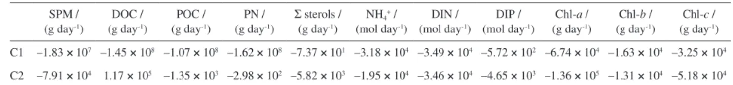
The flow rates calculated on a daily basis are given in Table 4 and indicate net export of materials to the inner shelf in both samplings, except for DOC in C2. Exports of DIN, Chl-b and Chl-c were of the same order in both
campaigns; those of DIP, Chl-a and sterols predominated
in C2 while SPM, DOC, POC and PN were more important in C1. DOC importation in C2 may derive from the inflow during high tide of organic carbon associated with the suggested algae bloom event prior to the sampling day and also from influence of the sewage outfall located closer to the bay mouth with respect to the sampling station. The widespread delivery of untreated sewage into the bay causes variability in chemical properties of the system and difficulties of source identification.
As the two samplings were performed in distinct conditions typically found during the dry and wet period,
Figure 8. Factor analysis including sterols in surface (S, in red), mid-depth (M, in blue) and bottom (F, in black) samples; (a) and (c) stand for C1 and (b) and (d) stand for C2 sampling.
obtained data on daily basis can be used for estimating the magnitude of the exchanges on an annual basis as necessary for comparison with literature data. The export rates to the inner continental shelf so far estimated are: 1.27 × 10⁴ kmol year-1 DIN; 9.52 × 10² kmol year-1 DIP; 2.65 × 10¹⁰ g year-1 DOC; 1.96 × 10¹⁰ g year-1 POC; and 2.96 × 10¹⁰ g year-1 PN.
Souza et al.83 report the following integrated flow rates for 24 rivers in the northeast and southeast coast of Brazil: average DIN ca. 3.0 × 10² kmol day-1 and DIP = 4.4 and 37 kmol day-1 in the months of September and December 2000, respectively. These flow rates are approximate since they were calculated based on published data (National Water Agency). Figueiredo et al.84evaluated the outputs of C and N from the Paraiba do Sul River (hydrographic basin: 22,000 km2, average drainage: 900 m3 s-1) to the Atlantic Ocean and found 48 × 109 g year-1 particulate carbon (PC), 83 × 109 g year-1 DOC and 8 × 10⁸ g year-1 PN. The data of the present work reveal that on a regional scale GB contributes with about 10% of the dissolved N and P that enters into the continental shelf through river inputs of the Northeast and Southeast Brazil. If compared to the Paraiba do Sul River estimates, GB contributes with an export of DOC of the same order of magnitude and with 24 times higher PN output.
The international program Land-Ocean Interactions in the Coastal Zone (LOICZ) produced numerous studies targeting nutrient flow rates to the oceans in coastal areas. Table 5 shows the results for nutrient flow rates from several systems in the Baltic Sea.85
Dupra86 estimated flow rates in the range of 102 to 106 kmol year-1 DIN and 102 to 105 kmol year-1 DIP for 30 ecosystems in the Southeast Asia region. Wepener,87 by using the LOICZ model, found the following average flow rates for the Nhlabane, Thukela and Mvote Estuaries, respectively: 0.076, 15, and 0.634 kmol day-1 for DIP and 1.7, 399, and 0.015 kmol day-1 for DIN. Arndt et al.,88 using mechanistic model, estimated for the Scheldt Estuary, Belgium, a DIN flow rate of the order of 105 kmol year-1. The GB exports of DIN and DIP are of the order of one thousandth of the outputs into the Baltic Sea, and are in the center of the flow rate range reported for the South Asia Sea. He et al.6 estimated a mangrove-derived POC flux of
5.3 × 10⁵ to 1.0 × 10⁶ kg year-1 POC from the Shark River into the Gulf of Mexico.
Meybeck89 estimated the following global nutrient transport to the oceans using data from the 1970s: 13 × 106 kmol year-1 (natural load) DIP; 26 × 106 kmol year-1 (natural + anthropic loads) DIP; 320 × 106 kmol year-1 (natural load) DIN; and 480 × 106 kmol year-1 (natural + anthropic loads) DIN. The comparison of these loads with the reported for the 1990s by Smith et al.90 of 21 × 106 kmol year-1 (natural load) DIP; 74 × 106 kmol year-1 (natural + anthropic loads) DIP; 400 × 106 kmol year-1 (natural load) DIN; and 1,350 × 106 kmol year-1 (natural + anthropic loads) DIN shows an increase of up to 3 times in the global nutrient anthropic load over the period of the 20 years so far considered. More recently, Liu et al.91 estimated the net global organic carbon input from rivers into the oceans as 0.4 Pg C year-1.
The estimated global nutrient loads from rivers are of 0.32-0.64 Tmol N year-1 for DIN and 13-27 Gmol P year-1 for DIP. The contribution of GB on a global scale may be estimated using these flow rates and turns out to be of 1.2 × 10⁻²% for organic carbon, 2.6 × 10⁻³% DIN and 4.7 × 10⁻³% DIP.
Conclusions
The present results show that GB comprises one of the most relevant systems in the southeastern Brazilian coast as
Table 4. Flow rates for SPM, DOC, POC, PN, Σ sterols, NH4+, DIN, DIP, Chl-a, Chl-b, Chl-c obtained on a daily basis for C1 and C2 samplings. Negative values represent transport from Guanabara Bay to the continental shelf
SPM / (g day-1)
DOC / (g day-1)
POC / (g day-1)
PN / (g day-1)
Σ sterols / (g day-1)
NH4+ / (mol day-1)
DIN / (mol day-1)
DIP / (mol day-1)
Chl-a / (g day-1)
Chl-b / (g day-1)
Chl-c / (g day-1)
C1 –1.83 × 10⁷ –1.45 × 10⁸ –1.07 × 10⁸ –1.62 × 10⁸ –7.37 × 101 –3.18 × 10⁴ –3.49 × 10⁴ –5.72 × 10² –6.74 × 10⁴ –1.63 × 10⁴ –3.25 × 10⁴
C2 –7.91 × 10⁴ 1.17 × 10⁵ –1.35 × 10³ –2.98 × 10² –5.82 × 10³ –1.95 × 10⁴ –3.46 × 10⁴ –4.65 × 10³ –1.36 × 10⁵ –1.31 × 10⁴ –5.18 × 10⁴
SPM: suspended particulate matter; DOC: dissolved organic carbon; POC: particulate organic carbon; PN: particulate nitrogen; DIN: dissolved inorganic nitrogen; DIP: dissolved inorganic phosphorus; Chl-a, Chl-b, Chl-c: chlorophylls a, b and c; C1: dry season campaign; C2: wet season campaign.
Table 5. Flow rates for DIN and DIP of some ecosystems of the Baltic Sea
Ecosystem DIN / (kmol year-1) DIP / (kmol year-1)
Lulealven 6.5 × 10⁴ 1.2 × 10³
Neva 4.3 × 10⁶ 1.2 × 10⁵
Gulf of Riga 5.8 × 10⁶ 7.0 × 10⁴
Curonian Lagoon 7.5 × 10⁵ 2.5 × 10⁴
Gulf of Gdansk 3.3 × 10⁶ 1.8 × 10⁵
Sczeczin Lagoon 6.3 × 10⁶ 6.3 × 10⁴
far as the export of organic carbon and nutrient species is concerned. The comparison of the obtained flow rates with regional and global data demonstrates the magnitude of potential impact on the biogeochemistry of the inner shelf. The major source of nutrient and productivity enrichment is sewage input derived from densely populated municipalities in the hydrographic basin.
The use of sterols and stable isotopes as markers of organic matter origin successfully indicated the system variability due to interaction with ocean waters, seasonality and tidal oscillations. The study shows that anthropogenic inputs to the bay are rapidly mineralized and used to produce autochthonous material, which is then exported to the inner shelf. Such POC, differently from the natural terrestrial organic carbon, is of high nutritional value and thus may contribute significantly to the ecology of the pelagic and benthic secondary producers in the shelf. Moreover, undesirable effects, such as red tides occurring in the open coastal area off Guanabara Bay and appearance of large bacteria community may result in indirect effects upon the health of the coastal oceans.
The discharge of raw or insufficiently treated sewage directly into estuaries is not unique of Rio de Janeiro but often occurs in developing as well as in developed countries. Therefore, the global impact of these sources on the carbon and nutrient cycles must be better quantified and understood.
Supplementary Information
Supplementary data are available free of charge at http://jbcs.sbq.org.br as PDF file.
Acknowledgments
The authors are grateful to Coordenação de Aperfeiçoamento de Pessoal de Nível Superior (CAPES) and Fundação de Amparo à Pesquisa do Estado do Rio de Janeiro (FAPERJ) for the financial support.
References
1. Bauer, J. E.; Cai, W. J.; Raymond, P. A.; Bianchi, T. S.; Hopkinson, C. S.; Regnier, P. A.; Nature 2013, 504, 61.
2. Baker, A. C.; Glynn, P. W.; Riegl, B.; Estuarine, Coastal Shelf Sci. 2008, 80, 435.
3. Canuel, E. A.; Cammer, S. S.; McIntosh, H. A.; Pondell, C. R.;
Annu. Rev. Earth Planet Sci. 2012, 40, 685.
4. Hobbie, J. E.; Estuarine Science: A Synthetic Approach to Research and Practice; Island Press: Washington, D.C.,
2000.
5. Salomons, W.; Kremer, H. H.; Turner, R. K.; Andreeva, E. N.; Arthurton, R. S.; Behrendt, H.; Burbridge, P.; Chen, C.-T. A.; Crossland, C. J.; Gandrass, J. In Coastal Fluxes in the Anthropocene; Crossland, C. J.; Kremer, H. H.; Lindeboom, H.;
Marshall Crossland, J. I.; Le Tissier, M. D. A., eds.; Springer: Berlin, 2005, ch. 4, p. 145.
6. He, D.; Mead, R. N.; Belicka, L.; Pisani, O.; Jaffé, R.; Org. Geochem. 2014, 75, 129.
7. Hedges, J. I.; Keil, R. G.; Mar. Chem. 1999, 65, 55.
8. Zimmerman, A.; Canuel, E.; Estuarine, Coastal Shelf Sci. 2001, 53, 319.
9. Zimmerman, A. R.; Canuel, E. A.; Mar. Chem. 2000, 69, 117.
10. Borges, A. C.; Sanders, C. J.; Santos, H. L.; Araripe, D. R.; Machado, W.; Patchineelam, S. R.; Mar. Pollut. Bull. 2009, 58,
1750.
11. Smith, V. H.; Schindler, D. W.; Trends Ecol. Evol. 2009, 24,
201.
12. Beukema, J.; Mar. Biol. 1991, 111, 293.
13. Parker, C. A.; O’Reilly, J. E.; Estuaries 1991, 14, 248. 14. Pennock, J. R.; Sharp, J. H.; Schroeder, W. W. In Changes in
Fluxes in Estuaries: Implications From Science to Management; Dyer, K. R.; Orth, R. J., eds.; Olsen & Olsen: Fredensborg, 1994, p. 139.
15. Doney, S. C.; Science 2010, 328, 1512.
16. Cai, W.-J.; Hu, X.; Huang, W.-J.; Murrell, M. C.; Lehrter, J. C.; Lohrenz, S. E.; Chou, W.-C.; Zhai, W.; Hollibaugh, J. T.; Wang, Y.; Nat. Geosci. 2011, 4, 766.
17. Berounsky, V. M.; Nixon, S. W.; Estuarine, Coastal Shelf Sci. 1985, 20, 773.
18. Braga, E. S.; Bonetti, C. V.; Burone, L.; Bonetti Filho, J.; Mar. Pollut. Bull. 2000, 40, 165.
19. Innamorati, M.; Giovanardi, F.; Sci. Total Environ. 1992,
235.
20. Kimor, B.; Sci. Total Environ. 1992, 871.
21. Niencheski, L.; Windom, H.; Sci. Total Environ. 1994, 149, 53. 22. Nixon, S. W.; Pilson, M. E.; The Estuary as a Filter; Academic
Press: Orlando, 1984.
23. Smith, S.; Veeh, H.; Estuarine, Coastal Shelf Sci. 1989, 29, 195.
24. Selman, M.; Greenhalgh, S.; Diaz, R.; Sugg, Z.; World Resources Institute 2008, 284, 1.
25. http://www.comitebaiadeguanabara.org.br accessed in February 2016.
26. Carreira, R. S.; Wagener, A. L.; Readman, J. W.; Estuarine, Coastal Shelf Sci. 2004, 60, 587.
27. Gonzalez, A. M.; Paranhos, R.; Andrade, L.; Valentin, J. L.;
Braz. Arch. Biol. Technol. 2000, 43, 493.
28. Wagener, A. L. R.; Quim. Nova 1995, 18, 534.
29. Rebello, A. L.; Ponciano, C.; Melges, L.; An. Acad. Bras. Cienc. 1988, 60, 419.
Farjalla, V. F.; Esteves, F. A., eds.; PPGE-UFRJ: Rio de Janeiro, 2001, p. 117.
31. Amador, E. S.; Baía de Guanabara e Ecossistemas Periféricos: Homem e Natureza; Reproarte Gráfica e Editora: Rio de Janeiro,
1997.
32. Japanese International Cooperation Agency (JICA); The study
on Recuperation of the Guanabara Bay Ecosystem;
JICA-Fundação Estadual de Engenharia de Meio Ambiente: Tokyo-Rio de Janeiro, 1994.
33. Kjerfve, B.; Ribeiro, C. H. A.; Dias, G. T. M.; Filippo, A. M.; Quaresma, V. S.; Cont. Shelf Res. 1997, 17, 1609.
34. Carreira, R. S.; Wagener, A. L.; Readman, J. W.; Fileman, T. W.; Macko, S. A.; Veiga, A.; Mar. Chem. 2002, 79, 207.
35. Diretoria de Hidrografia e Navegação (DHN); Cartas de Correntes de Maré: Baía de Guanabara, 1ª ed.; DHN: Niterói, 1974.
36. Grasshoff, K.; Kremling, K.; Ehrhardt, M.; Methods of Seawater Analysis; John Wiley & Sons: Bremen, 2009.
37. Parsons, T.; A Manual of Chemical and Biological Methods for Seawater Analysis; Pergamon Press: Oxford, 1984.
38. Jeffrey, S. W.; Humphrey, G. F.; Biochem. Physiol. Pflanz. 1975,
167, 191
39. Andrade, L.; Gonzalez, A.; Araujo, F.; Paranhos, R.;
J. Microbiol. Methods 2003, 55, 841.
40. Gasol, J. M.; Del Giorgio, P. A.; Sci. Mar. 2000, 64, 197. 41. http://www.epa.gov/osw/hazard/testmethods/sw846/
pdfs/3540c.pdf acessed in February 2016.
42. da Silveira, I. C. A.; Schmidt, A. C. K.; Campos, E. J. D.; de Godoi, S. S.; Ikeda, Y.; Rev. Bras. Oceanogr. 2000, 48, 171. 43. Ríos, A. F.; Resplandy, L.; García-Ibáñez, M. I.; Fajar, N.
M.; Velo, A.; Padin, X. A.; Wanninkhof, R.; Steinfeldt, R.; Rosón, G.; Pérez, F. F.; Proc. Natl. Acad. Sci. U. S. A.2015, 112, 9950.
44. Guenther, M.; Lima, I.; Mugrabe, G.; Tenenbaum, D. R.; Gonzalez-Rodriguez, E.; Valentin, J. L.; Braz. J. Oceanogr. 2012, 60, 405.
45. Frieder, C.; Nam, S.; Martz, T.; Levin, L.; Biogeosciences 2012,
9, 3917.
46. Fundação Estadual de Engenharia do Meio Ambiente (FEEMA);
Qualidade da Água da Baía da Guanabara - 1990 a 1997;
FEEMA: Rio de Janeiro, 1998.
47. Guenther, M.; Paranhos, R.; Rezende, C. E.; Gonzalez-Rodriguez, E.; Valentin, J. L.; Aquat. Microb. Ecol. 2008, 50, 123.
48. Moser, G. A. O.; Takanohashi, R. A.; Braz, M. C.; Lima, D. T.; Kirsten, F. V.; Guerra, J. V.; Fernandes, A. M.; Polley, R. C. G.;
Hydrobiologia2014, 728.
49. Redfield, A. C.; Ketchum, B. H.; Richards, F. A. In The Sea,
vol. 2; Hill, M. N., ed.; Intersci. Publ.: New York,1963, ch. 2. 50. Kalas, F. A.; Carreira, R. S.; Macko, S. A.; Wagener, A. L.;
Cont. Shelf Res. 2009, 29, 2293.
51. Organisation for Economic Cooperation and Development (OECD); Eutrophication of Waters, Monitoring assessment and control, Final Report; OECD: Paris, 1982.
52. Schwamborn, R.; Bonecker, S.; Galvão, I.; Silva, T.; Neumann-Leitão, S.; J. Plankton Res. 2004, 26, 983.
53. Villac, M. C.; Tenenbaum, D. R.; Biota Neotrop. 2010, 10, 271.
54. Azam, F.; Science1998, 280, 694.
55. Wagener, D. L. R; Bough, C.; de Figueiredo, L. M.; Carreira, R.; Wagener, K.; Chem. Ecol. 1992, 6, 19.
56. Chen, Z.; Li, Y.; Pan, J.; Cont. Shelf Res. 2004, 24, 1845.
57. Abril, G.; Estuarine, Coastal Shelf Sci. 2002, 54, 241. 58. Findlay, S.; Pace, M. L.; Lints, D.; Cole, J. J.; Caraco, N. F.;
Peierls, B.; Limnol. Oceanogr. 1991, 36, 268.
59. Goldman, J. C.; Caron, D. A.; Dennett, M. R.; Limnol. Oceanogr. 1987, 32, 1239.
60. Meyers, P. A.; Chem. Geol. 1994, 114, 289.
61. Carreira, R. S.; Wagener, A. D. L.; Mar. Pollut. Bull. 1998, 36, 818.
62. Cifuentes, L.; Coffin, R.; Solorzano, L.; Cardenas, W.; Espinoza, J.; Twilley, R.; Estuarine, Coastal Shelf Sci. 1996, 43, 781.
63. Summons, R. E. In Organic Geochemistry. Principles and Applications; Engel, M. H.; Macko, S., eds.; Springer: New York, 1993, ch. 1, p. 3.
64. Fogel, M. L.; Cifuentes, L. A. In Organic Geochemistry. Principles and Applications; Engel, M. H.; Macko, S., eds.;
Springer: New York, 1993, ch. 3, p. 73.
65. Meyers, P. A.; Tenser, G. E.; Lebo, M. E.; Reuter, J. E.; Limnol. Oceanogr. 1998, 43, 160.
66. Sachs, J. P.; Repeta, D. J.; Goericke, R.; Geochim. Cosmochim. Acta 1999, 63, 1431.
67. Schäfer, P.; Ittekkot, V.; Naturwissenschaften 1993, 80, 511.
68. Massone, C. G.; Wagener, A. L. R.; Abreu, H. M.; Veiga, A.;
Mar. Pollut. Bull. 2013, 73, 345.
69. Volkman, J. K.; Org. Geochem. 1986, 9, 83.
70. Leeming, R.; Ball, A.; Ashbolt, N.; Nichols, P.; Water Res. 1996, 30, 2893.
71. Duan, Y.; Org. Geochem. 2000, 31, 159.
72. Mudge, S.; Lintern, D. G.; Estuarine, Coastal Shelf Sci. 1999,
48, 27.
73. Barrett, S. M.; Volkman, J. K.; Dunstan, G. A.; LeRoi, J. M.;
J. Phycol. 1995, 31, 360.
74. Bianchi, T. S.; Canuel, E. A.; Chemical Biomarkers in Aquatic Ecosystems; Princeton University Press: Princeton, 2011.
75. Mudge, S. M.; Norris, C. E.; Mar. Chem. 1997, 57, 61. 76. Yoshinaga, M. Y.; Sumida, P. Y.; Wakeham, S. G.; Org.
Geochem. 2008, 39, 1385.
77. Robinson, N.; Eglinton, G.; Brassell, S.; Cranwell, P.; Nature 1984, 308, 439.
79. Santos, V. S.; Villac, M. C.; Tenenbaum, D. R.; Paranhos, R.;
Braz. J. Oceanogr. 2007, 55, 133.
80. Jeng, W.-L.; Huh, C.-A.; Appl. Geochem. 2001, 16, 95. 81. Grimalt, J. O.; Fernandez, P.; Bayona, J. M.; Albaiges, J.;
Environ. Sci. Technol. 1990, 24, 357.
82. Hites, R. A.; Elements of Environmental Chemistry;
Wiley-Interscience: Hoboken, 2007.
83. Souza, W.; Knoppers, B.; Balzer, W.; Leipe, T.; Geochim. Bras. 2003, 17, 130.
84. Figueiredo, R. O.; Ovalle, Á. R. C.; Rezende, C. E.; Martinelli, L. A.; Rev. Ambiente Agua 2011, 6, 7.
85. Wulff, F.; Rahm, L.; Hallin, A.-K.; Sandberg, J.; A Systems Analysis of the Baltic Sea; Springer: Berlin, 2001.
86. Dupra, V. C. In Coastal Fluxes in the Antropocene; Crossland,
C. J.; Kremer, H. H.; Lindeboom, H. J; Crossland, J. I. M.; Le Tissier, M. D. A., eds.; Springer-Verlag: Berlin, 2005, ch. 3, p. 95.
87. Wepener, V.; Water SA 2007, 33, 203.
88. Arndt, S.; Lacroix, G.; Gypens, N.; Regnier, P.; Lancelot, C.; J. Marine Syst. 2011, 84, 49.
89. Meybeck, M.; Am. J. Sci. 1982, 282, 401.
90. Smith, S. V.; Swaney, D. P.; Talaue-McManus, L.; Bartley, J. D.; Sandhei, P. T.; McLaughlin, C. J.; Dupra, V. C.; Crossland, C. J.; Buddemeier, R. W.; Maxwell, B. A.; BioScience 2003, 53, 235. 91. Liu, K.-K.; Atkinson, L.; Quinones, R.; Talaue-McManus, L.;
Carbon and Nutrient Fluxes in Continental Margins: A Global
Synthesis; Springer: Berlin, 2010.
Submitted: August 9, 2015