MODELING OF CRACK PROPAGATION IN A PREMOLAR TOOTH USING FINITE ELEMENT METHOD

(1)

(2)

GRADUATE PROGRAM IN STRUCTURAL ENGINEERING

Modeling of Crack Propagation in a Premolar Tooth using Finite

Element Method

Author: Maryam Ramezani

A thesis submitted to the Department of Structural Engineering of Universidade Federal de Minas Gerais (UFMG) in partial fulfillment of the requirements for the degree of Master of Science in Structural Engineering.

Adviser: Prof. Dr.Estevam Barbosa de Las Casas

Co-adviser: Prof. Dr.Osvaldo Luis Manzoli

Examination committee:

Prof. Dr. Estevam Barbosa de Las Casas

DEES – UFMG (Adviser)

Prof. Dr. Osvaldo Luis Manzoli

FEB – UNESP (Co-adviser)

Prof. Dr. Felicio Bruzzi Barros

DEES – UFMG (Internal Examiner)

Profa. Dr. Cláudia Machado de Almeida Mattos UFES (External Examiner)

Belo Horizonte, Brazil

(3)

vii, 46 f.enc.: il.

Orientador: Estevam Barbosa de Las Casas. Coorientador: Osvaldo Luis Manzoli.

Tese (doutorado) Universidade Federal de Minas Gerais, Escola de Engenharia.

Bibliografia: f. 43-46.

1. Engenharia de estruturas - Teses. 2. Biomecânica - Teses. 3. Dentes - Teses. 4. Bicúspides - Teses. 5. Método dos elementos finitos - Teses. I. Las Casas, Estevam Barbosa de. II. Manzoli, Osvaldo Luis. III. Universidade Federal de Minas Gerais. Escola de Engenharia. IV. Título.

(4)

(5)

i

The term cracked tooth syndrome refers to an incomplete fracture of a vital posterior tooth that

involves the dentine and occasionally extends into the pulp. To better understand the characteristics of

the cracked tooth syndrome, a cracked premolar tooth will be studied here by using computational

techniques. The first step for the analysis is the development of a 3D geometric model to serve as the

basis for a finite element analysis. This model, generated from a commercial code, will be exported to

a crack propagation program. By having the 3D model and choosing an appropriate crack propagation

technique that fits the problem, one can define the material properties and loading types and conduct

the crack propagation procedure under various loading conditions. A 2D model is fully studied while

some initial results are extracted for the 3D model. Finally, the numerically obtained results can be

compared with clinical results obtained from the literature.

(6)

ii

RESUMO

O termo síndrome do dente rachado refere-se a uma fratura incompleta de um dente posterior

vital que envolve a dentina e ocasionalmente se estende para a polpa. Para entender melhor as

características da síndrome do dente rachado, um dente pré-molar rachado será estudado aqui usando

técnicas computacionais. O primeiro passo para a análise é o desenvolvimento de um modelo

geométrico 3D para servir como base para uma análise de elementos finitos. Este modelo, gerado a

partir de um código comercial, será exportado para um programa de propagação de fissura. Ao ter o

modelo 3D e escolher uma técnica apropriada de propagação de fissuras que se encaixa no problema,

pode-se definir as propriedades do material e os tipos de carga e realizar o processo de propagação de

fissuras em várias condições de carga. Um modelo 2D é totalmente estudado enquanto alguns

resultados iniciais são extraídos para o modelo 3D. Finalmente, os resultados obtidos numericamente

podem ser comparados com os resultados clínicos obtidos a partir da literatura.

(7)

iii

To my parents and my brother for their kindness and encouragement in all journeys of my life. A very

special thanks to my lovely husband Mohammad, for his unconditional love that always support me to

overcome everything I am facing. I could have never imagined myself where I am at this moment

without their endless support.

I would like to thank my adviser Prof. Dr. Estevam Barbosa de Las Casas for giving me the opportunity

to work with him as an MSc student and guided me to learn too many new things in the field of

biomechanics. I also appreciate the guidance from my co-adviser Prof. Dr. Osvaldo Luis Manzoli for

giving me a chance to work with his code and perform the whole analyses under his support. In

addition, I would like to thank my Master committee members, Profa. Dr. Cláudia Machado de

Almeida Mattos and Prof. Dr. Felicio Bruzzi Barros for their constructive comments to have this final

version of my thesis.

To the members of the MECBIO laboratory in DEEs-UFMG, especially Veronika, and Prof. Osvaldo’s

group members, specifically Eduardo. I wish you all the best in your future. I also gratefully

acknowledge the fully and partially financial supports from the Brazilian research agencies CAPES

(Coordination for the Improvement of Higher Education Personnel), CNPq (National Council for

Scientific and Technological Developments) and FAPEMIG (Research Support Foundation of the

(8)

(9)

v

LIST OF FIGURES

Figure 1.1. Different types of cracked teeth (Internet, 2016) ... 1

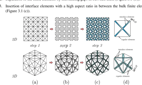
Figure 3.1. 2D and 3D mesh fragmentation process: (a) generation of the standard FE mesh to be fragmented; (b) separation of the finite elements (with an exaggerated scale factor for clarity); (c) insertion of interface elements (depicted in gray); and (d) detail of interface elements between regular elements (Manzoli et al, 2016). ... 12

Figure 3.2. Interface solid finite elements: (a) three-node triangular element and (b) four-node tetrahedron element (Manzoli et al, 2016). ... 13

Figure 3.3. Resulting discrete relation of the tension damage model ... 18

Figure 3.4. Representation of the different parts used in the tooth geometric model ... 18

Figure 3.5. Schematic of the dentin, enamel and restoration ... 19

Figure 3.6. Geometry of the dentin only (left) and enamel and dentin (right) without restoration ... 19

Figure 3.7. Schematic of the restoration area ... 19

Figure 3.8. Possible loading configuration as concentrated loads with different orientations. ... 20

Figure 3.9. Schematic of the meshed model ... 21

Figure 3.10. Displacement distribution, in millimeter. ... 22

Figure 3.11. Von-Mises stress component distribution (in MPa) ... 22

Figure 3.12. First principal stress component distribution (in MPa)... 22

Figure 3.13. Schematic of the boundary conditions, loading, and meshing model ... 23

Figure 3.14. First principal stress component and displacement distributions for 2D model in elastic analysis 24 Figure 4.1. CONROL_DATA input data. ... 25

Figure 4.2. GENERAL_DATA input data. ... 26

Figure 4.3. LOAD and BOUNDARY input data. ... 27

Figure 4.4. STRATEGY input data. ... 27

Figure 4.5. Fracture analysis procedure using the mesh fragmentation technique... 28

Figure 5.1. Schematic of the boundary conditions, loading, and meshing model ... 29

Figure 5.2. Distribution of displacements for lingual loading for 2D model in elastic analysis. ... 30

Figure 5.3. Distribution of displacements for buccal loading for 2D model in elastic analysis. ... 30

Figure 5.4. Distribution of displacements for lingual+buccal loading for 2D model in elastic analysis. ... 31

Figure 5.5. Distribution of principal stresses (in MPa) for lingual loading for 2D model in elastic analysis. .... 31

Figure 5.6. Distribution of principal stresses (in MPa) for buccal loading for 2D model in elastic analysis. .... 32

Figure 5.7. Distribution of principal stresses (in MPa) for lingual+buccal loading for 2D model in elastic analysis, with a different stress limits. ... 32

Figure 5.8. Position of the initial crack ... 33

Figure 5.9. Fracture results for lingual loading case, with different tensile strength values and a softening parameter of 85-408 m-1_{. ... 34}

Figure 5.10. Fracture simulation for buccal loading case, with different tensile strength and softening parameter of 85-408 m-1_{. ... 34}

Figure 5.11. Crack propagation path for lingual loading case, without any pre-existing crack. ... 35

Figure 5.12. Crack propagation path for lingual loading case, with a pre-existing crack. ... 36

Figure 5.13. Crack propagation path for buccal loading case, without any pre-existing crack. ... 36

Figure 5.14. Crack propagation path for buccal loading case, with a pre-existing crack at buccal side. ... 37

Figure 5.15. Crack propagation path for lingual+buccal loading case, for each loading sides, without any pre-existing crack. ... 37

Figure 5.16. Crack propagation path for lingual+buccal loading case, for each loading sides, with a pre-existing crack at lingual side. ... 38

Figure 5.17. Crack propagation path for lingual+buccal loading case, for each loading sides, with a pre-existing crack located at the bottom center of the cavity. ... 38

Figure 5.18. Total displacement distributions (mm) for 3D model in elastic analysis... 39

Figure 5.19. S1 stress distributions (MPa) for 3D model in elastic analysis... 40

(11)

(12)

1

1.1 Cracked Tooth Syndrome

The term cracked tooth syndrome (CTS) refers to an incomplete fracture of a vital posterior tooth

that involves the dentine and occasionally extends into the pulp (Cameron, 1964; Rosen, 1982; Lynch

et al, 2002). The symptoms are very variable, making it a notoriously difficult condition to diagnose.

The term was first introduced by Cameron in 1964 (Cameron, 1964), who noted a correlation between

restoration size and the occurrence of CTS. It was mentioned in the earlier literature of pulpal pain

resulting from incomplete tooth fractures. A more recent attempt to define the nature of this condition

describes it “as a fracture plane of unknown depth and direction passing through tooth structure that may progress to communicate with the pulp and/or periodontal ligament” (Ellis, 2001). The condition

presents mainly in patients aged between 30 years and 50 years (Hiatt, 1973; Snyder, 1976; Ellis et al,

1999). Men and women are equally affected (Türp et al, 1996). Mandibular second molars, followed

by mandibular first molars and maxillary premolars, are the most commonly affected teeth (Rosen,

1982; Braly et al, 1981). Two classic patterns of crack formation exist. The first occurs when the crack

is centrally located; the second is where the crack is more peripherally directed and may result in cuspal

fracture. Pressure applied to the crown of a cracked tooth leads to separation of the tooth components

along the line of the crack and causes pain.

1.2 Literature Survey

Teeth with or without restorations may exhibit CTS problem, but teeth restored with typical silver

alloy restorations are most susceptible. Figure 1.1 shows different types of cracked teeth.

(13)

There are different clinical studies during last decades dedicated to fracture analysis of teeth under

various conditions, from restored to root canal treated tooth. Siso et al. (2007) compared the cusp

fracture resistance of teeth restored with composite resins. They concluded that, for root filled

maxillary premolars, adhesive resin composite restorations increased the fracture resistance of the

buccal cusps. Goldberg et al. (2009) investigated the restoration of endodontically treated teeth and

concluded that a ferrule of 1-2 mm of tooth tissue coronal to the finish line of the crown significantly

improves the fracture resistance of the tooth and is more important than the type of the material of the

core and post.

Symptomatic, incompletely fractured posterior teeth can be a great source of anxiety for both

patient and dental operator. For the latter, there are some challenges associated with deriving the correct

diagnosis with an efficient and time management of cracked tooth syndrome cases. Banerji et al.

(2010a) discussed in detail the background of this syndrome including its epidemiology and diagnosis,

along with various considerations related to the CTS syndrome.

Banerji et al. (2010b) focused on the immediate and intermediate management, and provided a

definition for them, of cracked teeth, and also provided a detailed account of the application of both

direct and indirect restorations and restorative techniques used respectively in the management of teeth

affected by this complex syndrome. They concluded that “direct restorations with cuspal coverage, in

particular bonded composite restorations appear to be the most beneficial when considering prognostic

outcome of teeth restored for the purposes of incomplete posterior tooth fractures” (Banerji et al,

2010b).

A review of the literature to establish what evidence exists regarding the risk factors for cracked

teeth and their prevention, diagnosis, and treatment was made by Lubisich et al. (2010). They found in

the literature that almost all cracks are located in posterior teeth especially in mandibular molar. The

risk factors for a cracked tooth are multifactorial: natural causes (i.e. tooth form, age, and wear patterns)

or iatrogenic causes (i.e., tooth preparation). More controlled clinical studies are needed to determine

which treatment modalities are best suited for specific clinical situations. Recent research has shown

that cracks in teeth with no restorations, as well as fractures in the maxillary molars, appear more

frequently than once thought. Table 1.1 summarizes the data on the proportion of cracked teeth by

tooth type reported from 12 studies. This Table also shows the percentages of maxillary and mandibular

(14)

fractures. Averaging the results of the 12 studies investigated in (Lubisich et al., 2010) shows that once

a tooth is found to have a crack, 48% of cracked teeth are mandibular molars, 28% are maxillary

molars, 16% are maxillary premolars, 6% are mandibular premolars, and about 2% are other teeth.

Table 1.1. Proportion of cracked teeth by tooth type from 12 clinical studies (Lubisich et al., 2010)

Study author Tooth type Incidence rate (%) Total teeth % unrestored

Cameron (1964)

Mandibular molars 54

50 --- Maxillary molars 28

Mandibular premolars 2 Maxillary premolars 16

Other 0

Hiatt (1973)

100 35 Maxillary molars 19

Mandibular premolars 10 Maxillary premolars 1

Other 0

Talim and Gohil (1974)

--- --- Maxillary molars 22.5

Mandibular premolars 7.5 Maxillary premolars 25

Other 0

Cameron (1976)

Mandibular molars 66.7

102 --- Maxillary molars 23.5

Mandibular premolars 0 Maxillary premolars 9.8

Other 0

Abou-Rass (1983)

120 15.8 Maxillary molars 20.8

Mandibular premolars 0 Maxillary premolars 19.2 Other 14.2

Cavel et al. (1985)

(15)

Maxillary premolars 24.6

Other 0

Eakle et al. (1986)

Mandibular premolars 25.24 Maxillary premolars 5.83

Other 0

Lagouvardos et al. (1989)

Mandibular premolars 5 Maxillary premolars 28.5

Other 0

Bader et al. (2001)

Mandibular premolars 6.9 Maxillary premolars 20.4 Other 14.3

Brynjulfsen et al. (2002)

Other 0

Roh et al. (2006)

Other 0

Krell and Rivera (2007)

Other 0

Silva et al. (2012) studied and analyzed the effect of different load application devices on fracture

(16)

the type of load application device influences significantly the behavior of the teeth-restoration

complex during mechanical fracture resistance test.

Las Casas et al. (2014) presented a numerical predictive analysis of crack propagation which may

lead to fracture after root reconstruction. A scalar damage model based on the maximum principal

stress criterion was used to predict crack propagation. The parameters of the constitutive model were

the elastic properties, the tensile strength and the fracture energy of the material. They have concluded

that when weakened roots of endodontically treated teeth are treated with adhesive composite

reconstruction and post/core restoration, the risk of tensile damage to the root walls is higher with

stronger adhesive interfaces. Apparently, localized failures of the interface corresponding to peak stress

areas decrease the risk of damage to the root dentin walls. Lin et al. (2013) presented an investigation

of the failure risk for an endodontically treated restored premolar. They considered different crack

depths along with three different computer-aided design procedures. In addition, the ceramic onlay,

endo-crown, and conventional crown restorations are used to simulate the 3D FE models. The results

indicated that the stress values on the enamel, dentin, and luting cement for endo-crown restorations

exhibited the lowest values relative to the other two restoration methods.

The enamel of human teeth is generally regarded as a brittle material with low fracture toughness.

Consequently, the contributions of this tissue in resisting tooth fracture and the importance of its

complex have been largely overlooked. Experimental analysis of the tooth microstructure was done by

Yahyazadehfar et al. (2013) . Based on their analyses, they concluded that the fracture resistance of

enamel is both inhomogeneous and spatially anisotropic. The cracks initiating at the surface of teeth

may begin extension towards the dentin–enamel junction. They are deflected by the decussated rods

and continue growth about the tooth periphery, transverse to the rods in the outer enamel. This process

helps the dissipation of fracture energy and prevents cracks from propagating towards the dentin and

vital pulp.

Yahyazadehfar et al. (2014) studied the complex microstructures of tooth tissues, their roles in

resisting tooth fracture and the importance of hydration and aging on the fracture resistance of tooth

tissues is discussed. Their results show that both enamel and dentin are primarily extrinsically

toughened and it arises from the development of unbroken ligaments that act to shield the crack through

the development of bridging stresses. Finally, they concluded that the extrinsic toughening plays a

(17)

resistance of these materials is considerably lower under cyclic conditions in comparison to that in

quasi static loading.

Munari et al. (2015) studied and compared the areas of stress concentration in a 3D premolar tooth

model with anisotropic or isotropic enamel using the finite element method. Because tooth structures

are more resistant to compression, damage such as the formation of cracks and fracture of tooth

structure are likely to be caused by tensile stress from the eccentric contacts of unbalanced occlusion.

One of the main conclusion of this study was that the tensile stresses generated by the applications of

axial and oblique loads in isotropic models was larger than those in the anisotropic models, but the

stress distribution was similar.

Study of the behavior of thin interface regions between distinguished components of composite

structural members was conducted by Manzoli et al. (2012) using standard solid finite elements with a

very high aspect ratio. It has been shown that these elements present the same kinematics as the

continuous strong discontinuity approach. They concluded that their new technique helps users to

utilize very thin interfaces in a continuum framework, without the need of mesh refinement in the

interface area. In their numerical examples, the proposed damage constitutive model has shown that

the response of the continuum damage model becomes similar to the response that would be obtained

with a discrete relation.

Manzoli et al. (2016) used a new technique called “mesh fragmentation” for modelling cracks in

quasi-brittle materials based on the use of interface solid finite elements. “A tension damage

constitutive relation between stresses and strains is proposed to describe crack formation and propagation. The constitutive model is integrated using an implicit-explicit integration scheme to avoid convergence drawbacks, commonly found in problems involving discontinuities”. The results show that

the technique is able to predict satisfactorily the behavior of structural members involving different

crack patterns, including multiple cracks, without significant mesh dependency provided that

unstructured meshes are used.

In addition, there are various investigation reporting the loading magnitude for a tooth under

different loading conditions. Here are a summaries on the load values considered in various

investigations: a maximum load of 522 N was proposed in (Lyons et al, 1996; Proeschel et al, 2002)

(18)

N was conducted in (Palamara et al, 2002); a maximum biting force of 453 N was reported in (Litonjua

et al, 2004) based on experimental evaluation technique; a load of 380 N was applied on an implanted

premolar tooth (Hisam et al, 2015); and, a maximum load of 600 N was considered in (Misch, 2015)

applied on premolar tooth.

1.3 Motivation and Objectives

Finite Element Method (FEM) has been widely used for the numerical modeling of structural

problems (Hughes, 2000; Zienkiewicz et al, 2005). With the advent and popularization of

high-performance computers, the FEM is gaining more space in dental related applications over the past two

decades. Furthermore, improving the performance of the finite elements has been, in recent years,

important objects of studies and discussions. The use of computer-based FEM programs was greatly

facilitated with the development of pre- and post-processors rich interactive graphics capabilities,

allowing users with basic knowledge of geometry to easily work with them. On the other hand, there

are phenomena which performs the conventional form of the FEM cannot satisfactorily describe,

raising the development of new strategies for this purpose. Problems subjected to large deformation

and crack propagation, which require several changes in the discretization of the structure (remeshing),

are among those responsible to arise the interest for these new developments. The main focus of early

implementations of Finite Element (FE) models for discontinuity problems was defining meshes

conformed to discontinuity surfaces (Ingraea et al, 1985; Swenson et al, 1988). Not only generating a

mesh compatible with discontinuity surfaces is a challenging task in developing the finite element

models, but computed solutions of such models may also suffer from inaccuracy and

mesh-dependency. Moreover, redefining the mesh to capture the solution is inevitable for evolving

discontinuities. The remeshing becomes cumbersome, time consuming and a computationally

demanding task especially for three-dimensional problems.

Therefore, the mesh fragmentation technique proposed by Manzoli et al. (2016) is considered here

to overcome the associated problems with the finite element modeling.

There is a limited number of publications where the researchers tried to model crack growth in

teeth using the finite element method. Thus, one can obtain a realistic 3D model of a tooth and study

the crack propagation under various conditions. The modeling technique can be chosen from various

(19)

motivation and final goal of this project are “to predict the crack propagation in tooth structure using

a finite element analysis and special crack propagation techniques, as proposed by Manzoli et al. (2016)”.

1.4 Thesis outline

The remainder of the present text is organized as follows:

 Chapter 2: Presents an overview of quasi-brittle fracture mechanics formulations. It explains some basic formulations on linear elastic fracture mechanics and relevant texts

on quasi-brittle materials;

 Chapter 3: Provides the modeling technique and procedure and also some initial results

obtained by ABAQUS®_;

 Chapter 4: Presents the whole analysis methodology in detail, including the whole steps for fracture analysis using the mesh fragmentation technique;

 Chapter 5: Presents the results of fracture analysis of the premolar tooth using the mesh fragmentation technique;

(20)

9

This chapter is devoted to damage and fracture micromechanisms operating in the case when

monotonicallyincreasing forces are applied to engineering materials and components. According to

the amount of plasticdeformationinvolved in these processes, fracture events can be categorized as

brittle,quasi-brittle orductile.

Brittle fracture is typical for ceramic materials, where plastic deformation is strongly limited

across extendedranges of deformation rates and temperatures. In amorphous ceramics, it is simply

because ofa lack of any dislocations and, simultaneously, strong covalent and ionicinteratomic bonds.

Metallic materials or polymers exhibit brittle fracture only under conditions of extremely high

deformation rates, very low temperatures or extreme impurity concentrations at grain boundaries

(Pokluda et al, 2010). In thecase of astrong corrosion assistance, brittle fracture can also occur at very

small loading rates or even at aconstant loading (stress corrosion cracking).

Prior to cracking, quasi-brittle materials like concrete can, for many purposes, be modelled

sufficiently accurately as isotropic, linear-elastic. For instance, in a two-dimensional state of stress:

[ 𝜎𝑥𝑥 𝜎𝑦𝑦 𝜎𝑥𝑦

] = _{1 − 𝜈}𝐸 ₂[1 𝜈𝜈 1 00

0 0 1 2(1 − 𝜈)⁄ ] [ 𝜀𝑥𝑥 𝜀𝑦𝑦 𝛾𝑥𝑦

] (2-1)

where 𝜎_𝑥𝑥, 𝜎_𝑦𝑦, and 𝜎_𝑥𝑦 are normal stresses in x and y directions and shear stress in xy plane, respectively; Eis the Young’s modulus; 𝜈 is the Poisson ratio; and 𝜀_𝑥𝑥, 𝜀_𝑦𝑦, and 𝛾_𝑥𝑦 are strains in x

and y directions, and xy plane. When the major principal tensile stress exceeds the tensile strength or,

in more generally, when the combination of principal stresses violates a tension cut-off criterion, a

crack is initiated perpendicular to the direction of the principal stress. This embodies that in a sampling

point, where the stress, strain and history variables are monitored, the isotropic stress-strain relation is

replaced by an orthotropic law with the𝑛, s-axes the axes of orthotropy, where n is the direction normal

to the crack and s refers to the direction tangential to the crack. In a first attempt the orthotropic relation

can be defined as (Rashid, 1968):

[𝜎𝜎𝑛𝑛𝑠𝑠 𝜎𝑛𝑠

] = [0 0 00 𝐸 0 0 0 0] [

𝜀𝑛𝑛 𝜀𝑠𝑠 𝛾𝑛𝑠

(21)

where the orthotropic stress-strain relation has been set up in the coordinate system that aligns with the

axes of orthotropy. Eq. (2-2) shows that both the normal stiffness and the shear stiffness across the

crack are set equal to zero upon cracking. As a consequence, all effects of lateral contraction/expansion

also disappear.

If, for a plane-stress situation, 𝜎_𝑛𝑠= [𝜎_𝑛𝑛, 𝜎_𝑠𝑠, 𝜎_𝑛𝑠]𝑇 and 𝜀_𝑛𝑠= [𝜀_𝑛𝑛, 𝜀_𝑠𝑠, 𝛾_𝑛𝑠]𝑇 the secant stiffness

matrix 𝐷_𝑛𝑠𝑠 is defined as:

𝐷

𝑛𝑠𝑠 = [

0 0 0 0 𝐸 0

0 0 0] (2-3)

one can write the orthotropic elastic stiffness relation in the n, s-coordinate system as:

𝜎𝑛𝑠=

𝐷

𝑛𝑠𝑠 𝜀𝑛𝑠 (2-4)

Because of ill-conditioning, use of Eq. (2-2) may result in premature convergence difficulties.

Also, physically unrealistic and distorted crack patterns can be obtained, e.g. (Suidan et al, 1973). For

this reason a reduced shear modulus 𝛽𝐺 (0 ≤ 𝛽 ≤ 1) was reinserted in the model:

𝐷

𝑛𝑠𝑠 = [

0 0 0

0 𝐸 0

0 0 𝛽𝐺] (2-5)

where G is the shear modulus. The use of the so-called shear retention factor𝛽 not only reduces

the numerical difficulties, but it also improves the physical reality of fixed crack models, because it

can be thought of as a model representation of aggregate interlock. Most researchers simply adopt a

constant shear retention factor (𝛽 = 0.2 is a commonly adopted value) but sometimes a crack-strain

dependent factor is employed (Kolmar et al, 1984). The latter option is more realistic since the

capability of a crack to transfer shear stresses in mode-II decreases with increasing crack strain.

The fact that the stiffness normal to the crack in Eq. (2-5) is set equal to zero involves a sudden

drop of the tensile stress from the initial tensile strength 𝑓_𝑡 to zero upon crack initiation. Similar to the use of a zero shear retention factor, this may also cause numerical problems. The experimental

observation on quasi-brittle materials, like concrete, has led to the replacement of purely brittle crack

models by tension-softening models, in which a descending branch was introduced to model the

gradually diminishing tensile strength of concrete upon further crack opening. In a smeared context,

one can model this by inserting a normal reduction factor 𝜇 in the secant stiffness matrix:

𝐷

𝑛𝑠𝑠 = [

𝜇𝐸 0 0

0 𝐸 0

(22)

where, similar to the shear reduction factor 𝛽, the normal reduction factor 𝜇 can be a function of the

strain normal to the crack: 𝜇 = 𝜇(𝜀_𝑛𝑛) . A final refinement is given by the addition of Poisson coupling

after crack formation. Then, we arrive at the mode-I crack band formulation of Bazant and Oh (1983)

extended with mode-II shear retention:

𝐷

𝑛𝑠𝑠 = [

𝜇𝐸 1−𝜈2_𝜇

𝜈𝜇𝐸 1−𝜈2_𝜇 0

𝜈𝜇𝐸

1−𝜈2_𝜇 _1−𝜈𝐸2_𝜇 0

0 0 𝛽𝐺]

(2-7)

A typicalmicromechanism of brittle fracture is so-called cleavage,where the atoms aregradually

separated by tearing along the fracture plane in a very fast way(comparable to the speed of sound).

During the last 50 years, the resistance to unstable crack initiation and growth, i.e., the fracture

toughness, became a very efficient measure of brittleness or ductility of materials. In the case of

cleavage, this quantity can be simply understood in a multiscale context.The continuum linear–elastic

fracture mechanics approach were developed by Griffith (1921) and Irwin (1957), brought animportant

relationshipbetween the crack driving force Gfand the stress intensity factor KIas:

𝐺𝑓 =1 − 𝜈 2

𝐸 𝐾𝐼2 (2-8)

The 𝐺_𝑓 is defined also as the energy drop related to unit area of anew surface. This relation holds

for a straight front of an ideally flat crack under conditions of both the remote mode-I loading and the

plane strain. The energy necessary for creation of new fracture surfaces can be supplied from the elastic

energy drop of the cracked solid and/or from the work done by external forces (or the drop in the

(23)

– MODELING TECHNIQUE, PROCEDURE AND

INITIAL ANALYSES

This chapter gives detailed information on the tooth modeling technique and procedure and also

some initial analyses done using commercial code ABAQUS®_{. It contains the geometry information,}

material properties, loading types, boundary conditions, and meshing approach.

3.1 Modeling Technique

The main modeling technique comes from the mesh fragmentation procedure proposed by Manzoli

et al. (2016), so we just review the whole technique based on this reference. The proposed technique,

hereafter called mesh fragmentation technique, is based on the use of interface solid finite elements

with a high aspect ratio (2012), which are inserted in between standard (bulk) finite elements of a finite

element mesh. In this work, these interface elements are responsible for describing the crack formation

and propagation via an appropriate continuum damage model.

Figure 1 illustrates the main steps of the proposed mesh fragmentation technique for 2D and 3D

problems, which can be summarized as follows:

1. Generation of the standard FE mesh to be fragmented (Figure 3.1 (a)).

2. Separation of the finite elements by introducing gaps in between them (Figure 3.1 (b)).

3. Insertion of interface elements with a high aspect ratio in between the bulk finite elements (Figure 3.1 (c)).

Figure 3.1. 2D and 3D mesh fragmentation process: (a) generation of the standard FE mesh to be fragmented; (b) separation of the finite elements (with an exaggerated scale factor for clarity); (c) insertion

(24)

It is important to note in Figure 3.1 (b) that the gaps are in exaggerated scale for illustration. These

gaps are usually very small, with a thickness around 1% of the typical size of the regular elements.

Therefore, based on Manzoli et al. (2016), the assumption of 1% of the typical size of the regular

elements seemed to be a reasonable value, provided that the size of the regular elements has been

chosen to accurately capture the (elastic) stress field prior to the crack formation.

Triangular/tetrahedron finite elements are used for both the standard FE mesh and the interface

elements introduced during the fragmentation process (see Figure 3.1).

With the proposed strategy, cracks can only propagate along the interface elements. For problems

in which the region where cracks are expected is known a priori, the mesh fragmentation technique

may be applied only in the region of interest. This approach is very attractive since the steps mentioned

above are straightforward in implementation, giving place to an additional pre-processing stage. The

mesh fragmentation approach is completed by a continuum tension damage model formulated to

describe the formation and propagation of cracks along the interfaces.

3.1.1 Interface solid finite element

To describe the main features of the interface solid finite elements in 2D and 3D modeling,

standard three-node triangular finite element and four-node tetrahedrons, as illustrated in Figure 3.2,

are considered. The geometry of these elements can be characterized by the position of their nodes

according to a local Cartesian coordinate system (𝑛, 𝑠), defining the unit vector, n, normal to the

element base, and the height, h, given by the distance between node 1 and its projection on the element

base 1'.

Figure 3.2. Interface solid finite elements: (a) three-node triangular element and (b) four-node tetrahedron element (Manzoli et al, 2016).

Following the standard finite element approximations, the strain field of the solid finite element

(25)

𝜺 = 𝐵𝒅 (3-1)

where B is the strain–displacement matrix and d_{is the nodal displacement vector of the element.}

To show the similarity between the kinematics provided by these elements, when h tends to zero,

and that associated to the continuous strong discontinuity approach (CSDA), the strain tensor is divided

into two parts (Manzoli et al, 2012):

𝜺 = 𝜀̃ + 𝜀̂ (3-2)

where 𝜀̂ collects all the components of the strain tensor that depends on h, and 𝜀̃ contains the rest of

the components. Thus, the components that depend on h can be written as:

𝜀̂ =1_ℎ(𝑛 ⊗ [𝑢])𝑠

(3-3)

where (∙)𝑠 corresponds to the symmetric part of (∙), ⊗ denotes a dyadic product, and [𝑢] is a vector

that collects the components of the relative displacement between node 1 and its projection on the

element base 1. The total strain tensor, given by Eq. (3-2), can then be rewritten as:

𝜺 = 𝜀̃ +_ℎ1(𝑛 ⊗ [𝑢])𝑠

⏟

𝜀̂

(3-4)

As can be noted from this decomposition, when h tends to zero, the component 𝜀̃ remains bounded,

while the 𝜀̂ component is no longer bounded. As a consequence, in this situation, the element strains

are related almost exclusively to the relative displacement between node 1 and its projection on the

element base 1'. As described by Manzoli et al. (2012), in the limit situation (ℎ → 0), the relative

displacement [𝑢] becomes the measure of a displacement discontinuity (strong discontinuity), and the

structure of the strain field in Eq.

(3-4)

corresponds to the typical kinematics of the CSDA. Therefore,

based on the same concepts of the CSDA, it can be stated that bounded stress can be obtained from

unbounded strains by means of a continuum constitutive relation. The equivalence between the strain

field of the interface finite elements (when ℎ → 0) and the strong discontinuity kinematics is detailed

by Manzoli et al. (2012).

According to the local Cartesian coordinate system (n, s), depicted in Figure 3.2(a), the nodal coordinates of the 3-node triangular finite element are:

𝑥(1)_{= (ℎ, 𝑏} 2),

𝑥(2)_{= (0,0),}

𝑥(3)_{= (0, 𝑏)}

(3-5)

(26)

𝜀̃ =1_{𝑏 [} 0

1

2 (𝑢𝑛(3)− 𝑢𝑛(2))

1

2 (𝑢𝑛(3)− 𝑢𝑛(2)) (𝑢𝑠(3)− 𝑢𝑠(2))

] (3-6)

and

𝜀̂ =1_{ℎ [}⟦𝑢⟧𝑛 1 2⟦𝑢⟧𝑠

1

2⟦𝑢⟧𝑠 0

] (3-7)

where 𝑢_𝑛(𝑖)and 𝑢_𝑠(𝑖) are the components of the displacement of node i according to the (𝑛, 𝑠) system;

while ⟦𝑢⟧_𝑛= 𝑢_𝑛(1)− 𝑢_𝑛(1′) and ⟦𝑢⟧_𝑠= 𝑢_𝑠(1)− 𝑢_𝑠(1′)are the components of the relative displacement

⟦𝑢⟧. In the same way, the nodal coordinates of the 4-node tetrahedron finite element (see Figure 3.2(b))

according to a local Cartesian coordinate system (𝑛, 𝑠, 𝑡):

𝑥(1)_{= (ℎ, 𝑥}

𝑠(1), 𝑥𝑡(1)),

𝑥(2)_{= (0, 𝑥}

𝑠(2), 𝑥𝑡(2)),

𝑥(3)_{= (0, 𝑥}

𝑠(3), 𝑥𝑡(3)),

𝑥(4)_{= (0, 𝑥}

𝑠(4), 𝑥𝑡(4)).

Thus, the corresponding parts of the strain tensor, given by Eq. (3-4), can be expressed as:

𝜀̃ =_{𝐴 [}1 𝜀̃𝜀̃𝑛𝑛𝑛𝑠 𝜀̃𝜀̃𝑛𝑠𝑠𝑠 𝜀̃𝜀̃𝑛𝑡𝑠𝑡

𝜀̃𝑛𝑡 𝜀̃𝑠𝑡 𝜀̃𝑡𝑡

] (3-8)

and

𝜀̂ =1 ℎ

[

⟦𝑢⟧𝑛 1₂⟦𝑢⟧𝑠 1₂⟦𝑢⟧𝑡

1

2⟦𝑢⟧𝑠 0 0

1

2⟦𝑢⟧𝑡 0 0 ]

(3-9)

where

𝜀̃𝑛𝑛= 0,

𝜀̃𝑠𝑠=1_{2 [(𝑥}𝑡(3)− 𝑥𝑡(2))𝑢𝑠(4)+ (𝑥𝑡(2)− 𝑥𝑡(4))𝑢𝑠(3)+ (𝑥𝑡(4)− 𝑥𝑡(3))𝑢𝑠(2)],

𝜀̃𝑡𝑡= −1_{2 [(𝑥}𝑠(3)− 𝑥𝑠(2))𝑢𝑡(4)+ (𝑥𝑠(2)− 𝑥𝑠(4))𝑢𝑡(3)+ (𝑥𝑠(4)− 𝑥𝑠(3))𝑢𝑡(2)],

𝜀̃𝑛𝑠=1_{4 [(𝑥}𝑡(3)− 𝑥𝑡(2))𝑢𝑛(4)+ (𝑥𝑡(2)− 𝑥𝑡(4))𝑢𝑛(3)+ (𝑥𝑡(4)− 𝑥𝑡(3))𝑢𝑛(2)],

𝜀̃𝑛𝑡= −1_{4 [(𝑥}𝑠(3)− 𝑥𝑠(2))𝑢𝑛(4)+ (𝑥𝑠(2)− 𝑥𝑠(4))𝑢𝑛(3)+ (𝑥𝑠(4)− 𝑥𝑠(3))𝑢𝑛(2)],

𝜀̃𝑠𝑡=1_{4 [(𝑥}𝑡(3)− 𝑥𝑡(2))𝑢𝑡(4)+ (𝑥𝑡(2)− 𝑥𝑡(4))𝑢𝑡(3)+ (𝑥𝑡(4)− 𝑥𝑡(3))𝑢𝑡(2)− (𝑥𝑠(3)

− 𝑥𝑠(2))𝑢𝑠(4)− (𝑥𝑠(2)− 𝑥𝑠(4))𝑢𝑠(3)− (𝑥𝑠(4)− 𝑥𝑠(3))𝑢(2)],

(3-10)

A is the area of the element base with unit vector 𝑛; 𝑢_𝑛(𝑖), 𝑢_𝑠(𝑖) are 𝑢_𝑡(𝑖) the components of the

(27)

and ⟦𝑢⟧_𝑡 = 𝑢_𝑡(1)− 𝑢_𝑡(1′) are the components of the relative displacement ⟦𝑢⟧ between node 1 and the

point corresponding to its projection on the element base 1’ (𝑥(1′) = (0, 𝑥_𝑠(1), 𝑥_𝑡(1))).

3.1.2 Tension damage model

It is known that constitutive models based on the Continuum Damage Mechanics Theory (CDMT)

are appropriate todescribe the material degradation process due to crack propagation (Kachanov, 1986;

Lemaitre, 1992; Cervera et al, 1996; Murakami, 2012;). For this class of models, the mechanical

behavior of a damaged material is usually described by using the notion of the effective stress, together

with the hypothesis of mechanical equivalence between the damage and the undamaged material.

Here, the phenomenon of crack initiation and propagation through the interface solid finite

elements is described by a tension damage model. In the following, the main ingredients of this model

and the integration of the stress–strain relation using an implicit–explicit integration scheme are

detailed. The resulting discrete relation obtained when the interface element height, h, tends to zero is

also presented. The tension damage model is defined by the following constitutive relation:

𝝈 = (1 − 𝑑) ℂ: 𝜺⏟

𝜎̅ (3-11)

where 𝝈 is the nominal stress; 𝑑 ∈ [0,1] is the scalar damage variable; ℂ is the fourth order elastic

tensor; 𝜀 is the strain tensor; and the product ℂ: 𝜺 defines the effective stress tensor 𝝈̅. The damage

criterion defines the elastic domain and is given by:

𝜙 = 𝜎𝑛𝑛− 𝑞(𝑟) ≤ 0 (3-12)

where 𝜎_𝑛𝑛is the component of the stress normal to the base of the element (𝜎_𝑛𝑛= 𝒏. 𝝈. 𝒏), q and r

are the stress and strain like internal variables, respectively, and the function q(r) defines the softening

law, and 𝜙 is the damage criterion parameter.

To maintain the stresses bounded when the height tends to zero (ℎ → 0), all components of the

displacement jump must tend to zero if d = 0 (elastic regime). On the other hand, the damage variable

must tend to 1 in the inelastic regime with ⟦𝑢⟧ ≠ 0. Therefore, in the limit situation of ℎ → 0, the

interface element presents a rigid-damage behavior. Note that, before the stresses reach the damage

criterion all components of the displacement jump are precluded via penalization of 1 ℎ⁄ . This

penalization can be seen in the equation of the discrete constitutive model that emerges from the

continuum constitutive model. Note that the elastic stiffness of the discrete model is given by the

(28)

small values of h. This provides a rigid behavior, precluding the evolution of the displacement jump, before the stresses reach the damage criterion.

If the Poisson’s ratio is null (𝜈 = 0), the discrete relation can be expressed in terms of the Young’s

modulus, E, since:

4𝐺 3⁄ + 𝐾 = 𝐸 and 𝐺 = 𝐸 2⁄ (3-13)

where G is the shear modulus and K is the bulk modulus. For a monotonic increase (in mode-I) of

the normal displacement (⟦𝑢′⟧_𝑛 > 0, ⟦𝑢⟧_𝑠|_𝑡=0 = 0, ⟦𝑢⟧_𝑠 = ⟦𝑢⟧_𝑡 = 0), the evolution of the normal

stress becomes:

𝜎𝑛𝑛(⟦𝑢⟧𝑛) = (1 − 𝑑)1_{ℎ 𝐸}⟦𝑢⟧𝑛= {

1

ℎ 𝐸⟦𝑢⟧𝑛 𝑖𝑓 ⟦𝑢⟧𝑛≤ ⟦𝑢0⟧𝑛

(1 − 𝑑)1_{ℎ 𝐸}⟦𝑢⟧𝑛= 𝑞(𝑟) 𝑖𝑓 ⟦𝑢⟧𝑛> ⟦𝑢0⟧𝑛

(3-14)

with ⟦𝑢₀⟧_𝑛= ℎ 𝑞₀⁄𝐸. Assuming an exponential softening law of the form:

𝑞(𝑟) = 𝑞0𝑒𝒜ℎ(1−𝑟 𝑞⁄ )0 (3-15)

with 𝑞₀= 𝑓_𝑡,where 𝑓_𝑡is the tensile strength of the material and 𝒜 is the softening parameter, the

mode-I fracture energy, 𝐺_𝑓, i.e., the energy dissipated in a complete degradation of the interface element in

mode-I, is given as:

𝐺𝑓= ∫ 𝜎𝑛𝑛(⟦𝑢⟧𝑛)𝑑⟦𝑢⟧𝑛= ∫ 𝜎𝑛𝑛(⟦𝑢⟧𝑛)𝑑⟦𝑢⟧𝑛 ⟦𝑢0⟧𝑛

0 ∞

0

+∫_⟦𝑢∞ 𝜎_𝑛𝑛(⟦𝑢⟧_𝑛)𝑑⟦𝑢⟧_𝑛 0⟧𝑛

𝐺𝑓= (𝑓𝑡2ℎ 2 + 𝑓⁄ 𝑡2⁄𝒜) 𝐸⁄ .

(3-16) (3-17) (3-18)

When h tends to zero, the fracture energy tends to a non-null value given as:

𝐺𝑓= 𝑓𝑡 2

𝒜𝐸 (3-19)

from which one can define the softening parameter in terms of the material properties as:

𝒜 =_𝐺𝑓𝑡2

𝑓𝐸 (3-20)

Figure 3.3 illustrates the typical curve tension versus displacement jump (opening) normal to the

interface element, which is subjected to a uniaxial tension. Note that this discrete response corresponds

(29)

Figure 3.3. Resulting discrete relation of the tension damage model

3.2 Modeling Procedure

A geometric 3D finite element model of a premolar tooth was built. The model also includes a

representation of the mandible bone, which was based on tomography images. Six different materials

were considered: enamel, dentin, periodontal ligament, trabecular bone, cortical bone and resin.

Enamel and dentin are the basic tissues that constitute a sound human tooth. Resin is the restorative

materials. The periodontal ligament, which makes the link of the tooth with the mandible bone, is also

considered in the modeling process. Figure 3.4 illustrates the distribution of these materials in the

geometric domain. In addition, Figure 3.5 andFigure 3.6 are shown the enamel, dentin and restoration

representation in a closer view.

(30)

Figure 3.5. Schematic of the dentin, enamel and restoration

Figure 3.6. Geometry of the dentin only (left) and enamel and dentin (right) without restoration

The shape of the restoration is in accordance with the practical samples, i.e., a real specimen, and

similar to the one used in the work of Hamouda and Shehata (2011), Figure 3.7.

(a)real geometry (Hamouda and Shehata, 2011) (b) model geometry used in this study

(31)

The considered load was 180 N, according to (Cornacchia et al, 2010), divided in twelve point

loads, as shown in Figure 3.8. This load is only used to establish preliminary results for both 2D and

3D models. Also, the lateral external surfaces of the mandible bone were fixed in all directions

(representing clamped boundary conditions), as illustrated in Figure 3.4.

Figure 3.8. Possible loading configuration as concentrated loads with different orientations.

The mechanical properties of each material and tooth tissue are given in Table 3.1. The values for

the listed properties were taken from the literature, and the source chosen as reference directly affects

the obtained results, as there are no unique values given for the tissues.

Table 3.1. Mechanical properties of each tooth parts

Material Young’s modulus (GPa) Poisson’s ratio Tensile strength (MPa) Fracture Energy (J/m2₎

Enamel (Litonjua et al, 2004; Komatsu, 2010) 84.1 0.33 10-24 ---

Dentin (El Mowafy et al, 1986; Kinney et al, 1999; Kahler et al, 2003; Litonjua et al, 2004; Miguez et al, 2004; Mattos et al, 2012)

18.45 0.29 32-103 554-742

Composite Resin (Miguez et al, 2004; Chung et al,

2004; Thomaidis et al, 2013; Filtek website, 2014) 25.0 0.30 87 83

Periodontal Ligament (Misch et al, 1999; Pietrzak

et al, 2002) 0.000031 0.45 3.0 ---

Trabecular Bone (Van Staden et al, 2006; Baker

et al, 2010) 0.0962 0.30 140 ---

Cortical Bone (Reilly et al, 1974; Baker et al,

2010) 11.17 0.45 7.0 ---

Composite resin/Dentin interface (Phrukkanon et

(32)

3.3 Initial Analyses

This section describes an initial elastic analysis for two- and three-dimensional models using the

ABAQUS. The reason to perform the 3D analysis and then 2D analysis is that the tooth model was

first built in 3D, so it was decided to perform the initial 3D analysis first. After that, the 2D model was

created from the 3D model and thorough study were made on the 2D model.

3.3.1 3D Model

C3D4 element type (4-node tetrahedral element with 12 degrees of freedom) is used for all the domain.

Figure 3.9 shows the discretization model.

Figure 3.9. Schematic of the meshed model

Figure 3.10 shows the displacement distribution for premolar tooth in millimeters. The maximum

value occurs at the top of enamel, which was expected, and is around 0.028 mm.

Von-Mises and first principal stress distributions are shown in Figure 3.11 and Figure 3.12,

(33)

(a) enamel and dentin with restoration, mesial view. (b) enamel and dentin with restoration, distal view.

Figure 3.10. Displacement distribution, in millimeter.

Figure 3.11. Von-Mises stress component distribution (in MPa)

Figure 3.12. First principal stress component distribution (in MPa)

3.3.2 2D Model

A two-dimensional plane stress (with an out of plane thickness of 5 mm) model is created from a

section plane along the middle of 3D model. Here, an initial elastic analysis, similar to the 3D model,

(34)

boundary conditions, loading, and mesh schematic for the 2D analysis. Stress and displacement

distributions for this model are shown in Figure 3.14. As it can be seen from this figure, there are some

inconsistencies between 3D and 2D results, such as maximum values for both displacement and stress.

Those inconsistencies come from some out-of-plane loadings in 3D, because that model is not

symmetric along all axes (the symmetrical refers to the shape of tooth geometry, which is not

symmetric along all axes). Therefore, this anti-symmetric geometry can produce bending over one or

two axes when a similar loading is applied in the 3D model. Finally, it can be said that the 2D model

is not a reliable simplification for the actual problem, but it can be used to obtain preliminary results

in a simple model.

(35)

(a) S11 stress (in MPa) (b) Displacement (in mm)

Figure 3.14. First principal stress component and displacement distributions for 2D model in elastic analysis

A mesh sensitivity analysis was made for the 2D results presented here, for element sizes of 0.1

mm, 0.05 mm, and 0.025 mm. The maximum stress S11 for element sizes of 0.1 mm, 0.05 mm, and

0.025 mm were 30 MPa, 42.6 MPa, and 45.3 MPa, respectively. While, the maximum displacements

for element sizes of 0.1 mm, 0.05 mm, and 0.025 mm were 0.0774 mm, 0.0778 mm, and 0.0779,

respectively. As the displacement for these three element sizes were very close, stresses were

considered for mesh sensitivity evaluation. A quick look at the maximum stress values shows that from

element size of 0.05 mm to element size of 0.025 mm, there is only 6% difference. Therefore, the

element size of 0.05 mm can be represented a good mesh discretization and can deliver suitable results.

(36)

25

This chapter describes the used methodologies for analyzing the crack propagation in a tooth using

the mesh fragmentation technique. After providing the model geometry, the process starts by defining

the material properties, loading conditions, boundary condition, and finally discretizing the geometry.

A meshing software, the GiD pre- and post-processor software (GiD software, 2016), is used to

discretize the model. After having the discretized model, the input file for Matlab code must be

prepared, which includes the whole interface element and fragmentation formulation. The Matlab code

refers to the whole implementation regarding to the mesh fragmentation technique, developed and

implemented by Manzoli et al. (2012, 2016). This input file must be saved in ‘mfl’ format and it has

different parts in which all of them will be described here. The first part is the CONTROL_DATA, which

is shown in Figure 4.1.

Figure 4.1.CONROL_DATA input data.

As seen in Figure 4.1, the tag GEOMETRY is responsible to define the model dimension and its

type, 1 and 2 refer to 2D problems with plane strain and plane stress states, and 3 refers to the 3D

model. Under the DIMENSIONS section, the NPOIN, NELEM, NDPEL, NGAUS, and NSETS refer to

number of nodes, number of elements, number of nodes per element, number of Gauss points within

each element, and number of materials inside the geometry.

Then, geometry data including the elemental, nodal, and material properties are defined under the

GENERAL_DATA section, as shown in Figure 4.2. This data includes the element labels, their

connectivities and corresponding material sets, as well as nodal label and coordinates, and material

properties for each material set. In the material set definition, beside elastic modulus and Poisson’s

ratio, there are TYPE, MODEL, THICKNESS, and NGAUS where they refer to element type (2 for

triangular and 3 for tetrahedral), model type (1 for elastic model, 15 for model with interface elements

only in tension mode, and 21 for model with interface elements in both tension and shear modes),

model thickness, and number of Gauss points within each element, respectively. In the case of model

(37)

the softening parameter defined by Eq. (3-20). In addition, for model type 21 there are more two

additional parameters: FCULT, shear strength, and HBAC, the softening parameter in shear direction.

Figure 4.2.GENERAL_DATA input data.

Then, the INTERVAL_DATA section defines the number of steps to be solved (NSTEP) as well

as the incremental time of each step (DTIME). Figure 4.3 shows the input line for load and boundary

condition definitions. The load can be either POINT_LOAD or FACE_LOAD. In the case of

POINT_LOAD, a node label must be defined along with values of point load in different directions.

The BOUNDARY section defines the boundary condition, containing all nodes with their boundary

(38)

Figure 4.3.LOAD and BOUNDARY input data.

Figure 4.4 presents the required data for the analysis procedure, under the section STRATEGY. It

includes two tolerance parameter (TOL_NEWTON which is the Newton tolerance and

TOL_CONST_MODEL, the constitutive model tolerance), STRATEGY (1 for load control and 4 for

displacement control), DS which is incremental displacement to be used for controlling procedure,

NODE1 which is node to be used for displacement control approach, and DOF1 which is the direction

for displacement control approach.

Figure 4.4.STRATEGY input data.

After the input file preparation, it can be used to run an elastic analysis or insert the interface

element in between the elements, inside the region of interest, and perform the fracture analysis.

Figure 4.5 shows the steps to be done for the fracture modeling, from the model creation to the analysis

using the Matlab code. The 3D model came from a QCT (quantitative computed tomography)-scan

procedure to have both real geometry and material properties of a tooth. It was imported into the

Solidworks to create either 3D or 2D igs (Initial Exchange Specification) format files for the analysis.

Next, it was imported into the GiD, which was used for mesh generation and results visualizations.

After applying the material properties, boundary conditions, loading, and discretizing the model, an

initial input file can be extracted from the GiD, which has be modified to be usable by Matlab code

that is responsible to perform the fragmentation process. After that preparing the whole input file, a

(39)

conventional elements in the region of interest. At the end, the Matlab code is used for the analysis

based on mesh fragmentation technique.

(40)

- FRACTURE ANALYSIS USING MESH

FRAGMENTATION TECHNIQUE

5.1 Analyzing the 2D model

The 2D model is created from a section plane along the middle part of the 3D model. Figure 5.1

shows the geometry, boundary conditions, loading, and mesh schematic for the 2D analysis. There are

13,903 triangular elements (linear 3-node triangular elements) in the discretized model, with 5,419

elements for dentin; 774 elements for restoration; 1,017 elements for enamel; 1,261 elements for

periodontal ligament; 3,778 elements for cortical bone; and 1,654 elements for trabecular elements. In

this section, we describe the results for two different analyses: (1) an elastic analysis, and (2) a fracture

analysis, with different loading configurations (lingual, buccal, and lingual+buccal loadings cases

shown in Figure 5.1(a)). As we explained in chapter 1 and according to the literature, the loading

magnitude was set up to a maximum of 600 N.

(a) geometry and loading (b) mesh discretization.

(41)

5.1.1 Elastic Analysis

The stress and displacement distributions for this model, for the elastic analysis, are shown in

Figure 5.2 to Figure 5.4. The loading orientation has an important impact on both displacement and

stress distributions.

(a) x-direction (b) y-direction (c) total

Figure 5.2. Distribution of displacements for lingual loading for 2D model in elastic analysis.

(42)

Figure 5.4. Distribution of displacements for lingual+buccal loading for 2D model in elastic analysis.

An important fact is that the displacement distribution clearly shows the effect of various loading

cases. In order to study the elastic behavior of the tooth under aforementioned loading cases, the stress

distributions are shown in Figure 5.5 to Figure 5.7.

Figure 5.5. Distribution of principal stresses (in MPa) for lingual loading for 2D model in elastic analysis.

Figure 5.6 show the stress distributions for the buccal loading case. The stress concentrations are

a little far from the bottom side of the restoration, closer to the pulp boundaries. Error! Reference

(43)

(a) S1 (b) S2 (c) S3

Figure 5.6. Distribution of principal stresses (in MPa) for buccal loading for 2D model in elastic analysis.

Figure 5.7 shows the stress distribution for the case of lingual+buccal loading, aiming to clarify

the stress distributions near the bottom of the restoration, where a crack initiation might occur. The

stresses are mainly concentrated at the loading points, which they are expected. Other than these points,

the stress distributions are almost the same for the lower bottom corners of the restoration area.

Figure 5.7. Distribution of principal stresses (in MPa) for lingual+buccal loading for 2D model in elastic analysis, with a different stress limits.

5.1.2 Fracture Analysis

After the elastic analyses, interface elements are inserted in between the elements of dentin to

model the crack propagation in the dentin. These interface elements were inserted also between dentin

(44)

failure between these two parts during the crack propagation process. In addition, two different cases

were modeled: dentin with and without a pre-existing crack at different positions: lingual, buccal, and

central as shown in Figure 5.8 (with a length of 0.3 mm). Similar to the elastic analyses, three different

loading cases are also considered here to see the behavior of crack propagation in the dentin.

Figure 5.8. Position of the initial crack

As mentioned in chapter 4, besides elastic modulus and Poisson’s ratio, there are other parameters

that must be defined for those parts that contain interface elements: tensile strength and the softening

parameter. The tensile strength (FTULT) can be obtained from Table 3.1. The softening parameter

(HBAT) can be also calculated using Eq. (3-20) along with use of tensile strength, fracture energy and

elastic modulus from Table 3.1. Since the interface elements were only inserted in the dentin region,

let’s consider an average value for both tensile strength and fracture energy from Table 3.1: tensile

strength equal to 70 MPa and fracture energy equal to 650 N.m. Then, the HBAT would be equal to

408 m-1. Let’s first start to model the crack initiation _{and propagation in the dentin with these}

parameters with different loading conditions. Figure 5.9 and Figure 5.10 show the frature analysis for

the lingual and buccal loading cases with tensile strength of 32-70 MPa and a softening parameter of

85-408 m-1 _{(with an average fracture energy of 648 J/m}2_).

(45)

(b) With tensile strength of 50 MPa

(c) With tensile strength of 70 MPa

Figure 5.9. Fracture results for lingual loading case,with different tensile strength values and a softening parameter of 85-408 m-1_.

(a) With tensile strength of 32 MPa

(b) With tensile strength of 50 MPa

(c) With tensile strength of 70 MPa

Figure 5.10. Fracture simulation for buccal loading case,with different tensile strength and softening parameter of 85-408 m-1_.

According to Figure 5.9 and Figure 5.10, for the tensile strength value of 70 MPa, which is the

average values obtained from Table 3.1, there is no crack propagation for both lingual and buccal

(46)

loading value of 750N. For the tensile strength value of 50 MPa, there is a small crack propagation for

lingual loading of 600N, while for buccal loading of 600N there is no crack propagation. Finally, for

the tensile strength value of 32 MPa, we can see a quite big crack propagation for lingual loading equal

to 600N, but a small amount of crack propagation ocuured for buccal loading with the same loading

value. Therefore, it can be said that under current loading configurations and with an average values

for tensile strength and fracture energy, the restored tooth does not experience any major crack propagation. But, a value of 32 MPa is considered as the tensile strength value of the dentin in this research, for the failure point of the interface elements in the dentin part ro conduct a fruther fracture analysis. Although this value is the smallest value from Table 3.1, but it is choosed to study the fracture path under various loading conditions, while the results for the bigger values were also shown in the previous figures.

Therefore, the fracture path from different loading cases along with various pre-existing crack

positions, as well as model without any crack are shown in Figure 5.11 to Figure 5.17. The models

without cracks are analyzed in order to verify whether any crack would be initiated under different

loading orientations and various loading magnitudes. Then, for each loading cases, a corresponding

crack position will be inserted in the model. As an example, for lingual loading the lingual crack is

placed in the model. However, for lingual+buccal loading case, all the three pre-existing cracks are

placed in the model and their propagation behavior is studied separately.

(47)

Figure 5.12. Crack propagation path for lingual loading case, with a pre-existing crack.

(48)

Figure 5.14. Crack propagation path for buccal loading case, with a pre-existing crack at buccal side.

(49)

Figure 5.16. Crack propagation path for lingual+buccal loading case, for each loading sides, with a pre-existing crack at lingual side.

(50)

As it can be seen from previous figures, the lingual and lingual+buccal loading cases have shown

some bigger crack propagation paths, mainly due to their loading configuration as well orientation

regarding to the applied load surface, i.e., the restoration surface. The realistic loading value for a tooth

was chosen up to a maximum of 600N, from the literature. Therefore, all the crack propagation until

the loading of 600N is acceptable and can be considered more close to the realistic situation. However,

the bigger load magnitudes were shown as well in order to demonstrate the crack propagation behavior

under other less common loading conditions.

5.2 Elastic Analysis of the 3D Model

A preliminary 3D elastic analyses were also made for the whole tooth, using both Abaqus and

Matlab written program. The Abaqus results are used to validate the 3D elastic analysis with the Matlab

program. Figure 5.18 and Figure 5.20 show the displacement and first principal stress distributions,

obtained by Abaqus and Matlab program. As it can be seen from these two figures, the preliminary

elastic results from Matlab program are very close to those one obtained by Abaqus. Therefore, this

3D model can be used to conduct further elastic 3D analysis and 3D fracture analysis as well.

(a) Abaqus model, mesial view. (b) Abaqus model, distal view.

(c) GiD model solved in Matlab code, mesial view. (d) GiD model solved in Matlab code, distal view.

(51)

(a) Abaqus model, mesial view. (b) Abaqus model, distal view.

(c) GiD model solved in Matlab code, mesial view. (d) GiD model solved in Matlab code, distal view.

Figure 5.19. S1 stress distributions (MPa) for 3D model in elastic analysis

(a) (b)

MODELING OF CRACK PROPAGATION IN A PREMOLAR TOOTH USING FINITE ELEMENT METHOD