Numerical Study of Freezing Droplets

Faculdade de Engenharia

Numerical Study of Freezing Droplets

Leandro Barbosa Magalhães

Dissertação para obtenção do Grau de Mestre em

Engenharia Aeronáutica

(ciclo de estudos integrado)

Orientador: Prof. Doutor André Rodrigues Resende da Silva

iii

Acknowledgments

First and foremost I would like to take this opportunity to express my gratitude to my parents for their encouragement and support during my time at the University.

I would also like to thank my supervisor, Professor André Silva for his guidance throughout the development of this work, for his ability of solving apparent difficult questions with simple solutions and for his availability for every problem I had, which sometimes had nothing to do with this dissertation.

For last I wat to thank my colleague and friend Eduardo Antunes for his help with the idiosyncrasies of the FORTRAN computing language.

v

Resumo

O seguinte documento centra-se no estudo físico de processos de congelamento que se tornaram de extrema importância em engenharia aeronáutica. As causas mais comuns de danos estruturais em aeronaves devem-se a mudanças climatéricas como relâmpagos e o congelamento do bordo de ataque das asas ou das empenagens. O gelo espalha-se em direção ao bordo de fuga, afetando uma maior percentagem da superfície sustentadora em causa. Como resultado, surge uma necessidade de estudar e adaptar os modelos físicos e matemáticos existentes para uma melhor aproximação a situações reais, no sentido de uma diminuição da ocorrência de acidentes e incidentes resultantes deste tipo de fenómenos, contribuindo assim para melhores condições de aeronavegabilidade.

As previsões teóricas foram comparadas com dados experimentais e a análise numérica foi conduzida para a obtenção de uma melhor compreensão de processos de transmissão de calor e massa sob diferentes condições de humidade.

Palavras-chave

vii

Resumo alargado

O documento seguinte dedica-se ao estudo físico de processos de congelamento que se tornaram de extrema importância em engenharia aeronáutica no sentido de garantir melhores condições de aeronavegabilidade.

As causas mais comuns de danos estruturais em aeronaves são originadas por fatores climatéricos com relâmpagos e ao congelamento de superfícies sustentadoras como asas ou empenagens. A formação de gelo numa destas superfícies (no bordo de ataque) expande-se em direção ao bordo de fuga, a temperaturas abaixo de 0ºC, afetando uma maior percentagem da superfície, diminuindo a sustentação. Existe assim uma necessidade de incorporar e adaptar os modelos existentes para uma maior aproximação a situações reais. Uma revisão bibliográfica em que são abordados os princípios físicos de maior importância para este trabalho foi realizada tendo em conta várias aproximações matemáticas, com as suas vantagens e desvantagens e as condições segundo as quais se torna pertinente a sua aplicação num código de Dinâmica de Fluidos Computacional.

Numa segunda fase, modelos matemáticos representativos de várias situações que envolvem processos de congelamento são apresentados. Neste sentido, as previsões teóricas foram comparadas com dados experimentais para a validação do modelo numérico e para uma melhor compreensão dos processos físicos inerentes ao processo, como é o caso da transmissão de calor e massa sob diferentes condições de humidade.

ix

Abstract

The present work is devoted to the numerical study of freezing processes which have become of major importance in aeronautical engineering. The most common causes of structural damage to aircrafts result from climacteric changes such as lightning strikes and icing of the wing’s leading edges or empennage, which turns the smooth airflow over the wings into turbulent. At subzero temperatures, icing spreads from the leading to the trailing edge, affecting a greater percentage of the wings.

As a result there is a need to study and adapt existing physical and mathematical models to achieve a better approximation to real life situations in order to mitigate the occurrence of incidents and accidents involving aircraft for a better continuous airworthiness.

The theoretical predictions are compared against experimental data and the numerical analysis is conducted to provide insight into heat and mass transfer processes under several humidity conditions.

Keywords

xi

Table of Contents

ACKNOWLEDGMENTS ... III RESUMO ... V RESUMO ALARGADO ... VII ABSTRACT ... IX LIST OF FIGURES ... XIII LIST OF TABLES ... XV NOMENCLATURE ... XVII 1. INTRODUCTION ... 1 1.1.INTRODUCTION ... 1 1.2.OVERVIEW ... 3 2. BIBLIOGRAPHIC REVIEW ... 5 2.1.INTRODUCTION ... 5 2.2.PHYSICAL PHENOMENA ... 6 2.3.THE STEFAN PROBLEM ... 7

2.3.1. The Neumann solution ... 10

2.4.DENSITY CONSIDERATIONS ... 12

2.5.APPROXIMATIONS ... 13

2.5.1. Analytical approximations ... 14

2.5.1.1. Quasistationary approximation (Alexiades et al 1993) ... 14

2.5.1.2. Megerlin method (Alexiades et al 1993) ... 14

2.5.1.3. Heat balance integral method (Sethian et al 1993 & Lunardini 1981) ... 15

2.5.1.4. Perturbation method (Alexiades et al 1993) ... 15

2.5.2. Numerical approximations (Caginalp et al 1991 and Fix et al 1988) ... 15

2.5.2.1. Enthalpy formulation (Smith 1981) ... 18

3. MATHEMATICAL MODELS ... 21

3.1.INTRODUCTION ... 21

3.2.HEAT AND MASS TRANSFER ON A SYSTEM OF FREE FALLING DROPS ... 21

3.3.FOUR PHASE FREEZING WITH SUPERCOOLING ... 28

3.4.INITIAL CONDITIONS AND FLOW CONFIGURATION ... 33

4. RESULTS AND DISCUSSION ... 35

4.1.INTRODUCTION ... 35

4.2.INFLUENCE OF VARIABLE DROP DIAMETER ON THE FREEZING PROCESS ... 35

4.3.INFLUENCE OF VARIABLE HUMIDITY RATIO ON THE FREEZING PROCESS ... 40

4.3.SUMMARY ... 44

5. CONCLUSIONS AND FUTURE WORK ... 45

6. REFERENCES ... 47

ATTACHMENT 1 – EXTENDED ABSTRACT ACCEPTED FOR THE CEM 2016 ... 51

xiii

List of figures

FIGURE 1.1.EFFECT OF ICING ON AN AIRCRAFT WING,DILLINGHAM 2010 ... 1

FIGURE 2.1.NORMAL COOLING (A) VS SUPERCOOLING (B),ALEXIADES ET AL 1993 ... 7

FIGURE 2.2.TWO PHASE STEFAN PROBLEM,ALEXIADES ET AL 1993 ... 8

FIGURE 3.1.TECHNIQUES FOR THE STUDY OF SINGLE DROPS ... 21

FIGURE 3.2.HEAT AND MASS BALANCE OF A COLUMN OF AIR IN A DIFFERENTIAL ELEMENT ... 23

FIGURE 3.3.FLOWCHART FOR THE CALCULATION OF THE RATE OF COOLING OF A SYSTEM OF DROPS IN FREE FALL 27 FIGURE 3.4.MAIN FACTORS OF THE NUMERICAL SOLUTION ... 28

FIGURE 3.5.GENERIC REPRESENTATION OF A FOUR PHASE FREEZING PROCESS,HINDMARSH ET AL 2003 AND TANNER ET AL 2011 ... 29

FIGURE 3.6.COMPUTATIONAL DOMAIN ... 34

FIGURE 4.1.VARIATION ON DROPS’ TEMPERATURE FALLING THROUGH THE AIR FOR A DIAMETER OF 3 MM AND HUMIDITY RATIO OF 0.36 ... 36

FIGURE 4.2.VARIATION ON DROPS’ TEMPERATURE FALLING THROUGH THE AIR FOR VARIABLE DROP DIAMETER AND HUMIDITY RATIO OF 0.36 ... 37

FIGURE 4.3.VARIATION ON DROPS’ TEMPERATURE FALLING THROUGH THE AIR FOR VARIABLE DROP DIAMETER AND HUMIDITY RATIO OF 0.29 ... 38

FIGURE 4.4.VARIATION ON DROPS’ TEMPERATURE FALLING THROUGH THE AIR FOR VARIABLE DROP DIAMETER AND HUMIDITY RATIO OF 0.52 ... 38

FIGURE 4.5.VARIATION ON DROPS’ TEMPERATURE FALLING THROUGH THE AIR FOR VARIABLE DROP DIAMETER AND HUMIDITY RATIO OF 1. ... 39

FIGURE 4.6.VARIATION ON DROPS’ TEMPERATURE FALLING THROUGH THE AIR FOR A DIAMETER OF 3 MM AND VARIABLE HUMIDITY RATIO ... 40

FIGURE 4.7.VARIATION ON DROPS’ TEMPERATURE FALLING THROUGH THE AIR FOR A DIAMETER OF 4 MM AND VARIABLE HUMIDITY RATIO ... 41

FIGURE 4.8.VARIATION ON DROPS’ TEMPERATURE FALLING THROUGH THE AIR FOR A DIAMETER OF 5 MM AND VARIABLE HUMIDITY RATIO ... 42

FIGURE 4.9.VARIATION ON DROPS’ TEMPERATURE FALLING THROUGH THE AIR FOR A DIAMETER OF 6 MM AND VARIABLE HUMIDITY RATIO ... 43

xv

List of tables

TABLE 1.1.ICING AND WINTER WEATHER-RELATED INCIDENT REPORTS FOR LARGE COMMERCIAL AIRPLANES BY

CATEGORY OF INCIDENT,1998 TO 2007,DILLINGHAM 2010 ... 2

TABLE 2.1.OVERVIEW OF THE MOST COMMON ASSUMPTIONS ON THE STEFAN PROBLEM,ALEXIADES ET AL 1993 .... 9

TABLE 3.1.CONSTANTS OF THE SUTHERLAND RELATIONS ... 31

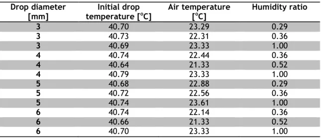
TABLE 3.2.VALUES FOR DROP DIAMETER, INITIAL DROP TEMPERATURE, AIR TEMPERATURE AND HUMIDITY RATIO.. 33

TABLE 4.1.INITIAL PROPERTIES FOR THE SIMULATION OF A HUMIDITY RATIO 0F 0.36 ... 37

TABLE 4.2.INITIAL PROPERTIES FOR THE SIMULATION OF A HUMIDITY RATIO 0F 0.36 ... 37

TABLE 4.3.INITIAL PROPERTIES FOR THE SIMULATION OF A HUMIDITY RATIO 0F 0.52 ... 39

TABLE 4.4.INITIAL PROPERTIES FOR THE SIMULATION OF A HUMIDITY RATIO 0F 1 ... 39

TABLE 4.5.INITIAL PROPERTIES FOR THE SIMULATION OF A DIAMETER OF 3 MM ... 41

TABLE 4.6.INITIAL PROPERTIES FOR THE SIMULATION OF A DIAMETER OF 4 MM ... 42

TABLE 4.7.INITIAL PROPERTIES FOR THE SIMULATION OF A DIAMETER OF 5 MM ... 43

XVII

Nomenclature

A droplet surface area B model constant C model constant CD drag coefficient

cL specific heat conductivity of liquid

cS specific heat conductivity of solid

Cpd drop specific thermal capacity

Cp water specific heat

𝐶𝑝𝛾 semi solid drop heat capacity

Cpl liquid drop heat capacity

Cps solid drop heat capacity

d drop diameter

𝑑ℎ𝑓 water enthalpy variation

𝑑𝑊 humidity variation within the control volume E emissivity

D mass diffusivity

Dvg gas or vapor thermal diffusivity

G correction factor

ℎ𝑐 convective heat transfer coefficient

ℎ𝑑 convective mass transfer coefficient

ℎ𝑓𝑔 water vaporization enthalpy

Kd heat conduction inside the drop

KL thermal conductivity in liquid

kS thermal conductivity in solid

L latent heat Le Lewis number

Lf latent heat due to crystallization

𝑚𝑎 air mass flow

𝑚𝑤 water mass flow

Nu Nusselt number PL Navier-Stokes tensor

Pr Prandtl number 𝑞𝐿 conductive heat flow

qh convective heat flow

qm mass heat flux

XVIII

Tm melt temperature/ phase change temperature

Tn nucleation temperature (empiric value)

Ts Temperature of the drop completely solidified

U drop velocity 𝑣⃗ velocity field Vd drop volume

Vr drop-gas relative speed

𝑊𝑠 Saturation humidity rate

𝑊∞ environment humidity rate

Greek symbols ρL liquid density ρS solid density Ν kinematic viscosity µ dynamic viscosity τ time 𝜎 Stefan-Boltzmann constant 𝛼 thermal diffusivity 𝜃 model constant 𝜀 total energy 𝜉 Similarity variable Acronyms

SIS Smart Icing Systems IPS Ice Protection System IMS Ice Management System NASA North American Space Agency

PCM Phase Change Material PDE Partial Differential Equation

XIX

FDE Finite difference Equation CFL Courant-Friedrichs-Lewy SOR Successive Over Relaxation

1

1. Introduction

1.1. Introduction

The present work is devoted to the numerical study of freezing processes which have become of major importance in aeronautical engineering. According to Caliskan and Hajiyev (2013), the most common causes of structural damage to aircrafts due to climacteric changes are the result of lightning strikes and icing at the wing’s leading edge or empennage.

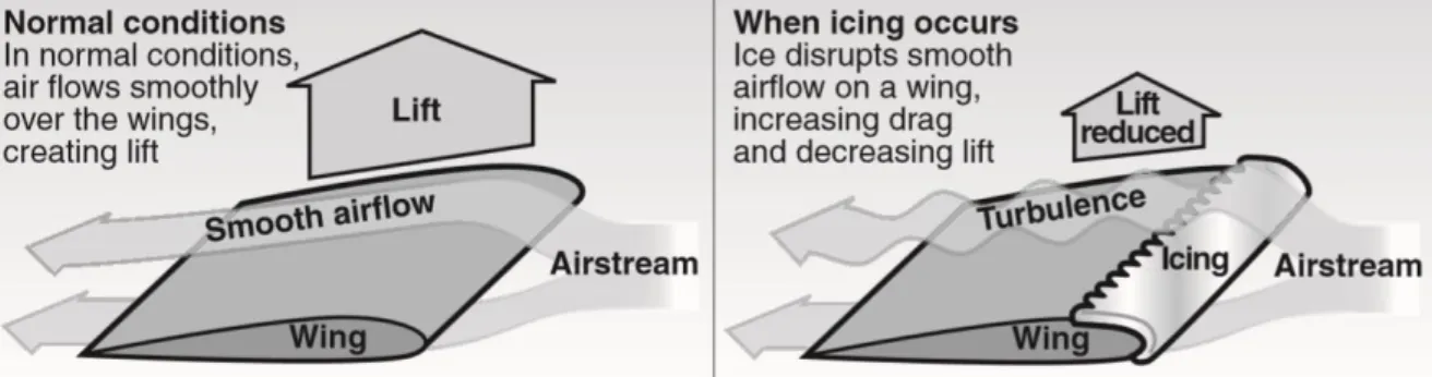
The icing of a wing’s leading edge turns the smooth airflow over the wing into a turbulent one, decreasing lift and increasing drag as seen in figure 1.1. At temperatures below zero, icing spreads to the trailing edge, affecting more of the wing.

Figure 1.1. Effect of icing on an aircraft wing, Dillingham 2010

Overall, icing has a negative effect on the aircraft’s aerodynamic performance, especially during take-off and landing and anti-icing systems on modern aircrafts make use of the heat exhausted from the engines, to prevent the ice from forming, which increases fuel consumption and in turn the operational costs of the aircraft. As a result, SIS (Smart Icing Systems) have been the focus of many studies.

SIS measure the ice accretion with the aircraft performance degradation and then the information is transmitted, in order to control the Ice Protection System (IPS) and if necessary to adjust the flight controls to the situation, coordinated with the flight crew.

Ice accretion can be divided into several categories, depending on the phenomenon responsible for them – the initial ice accretions on the lifting surfaces before or after anti-icing systems are deployed, which can be underestimated or neglected; runback or ridge ice accretions after the IPS is deployed, for the fact it reduces the aerodynamic effectiveness of the control surfaces; shaped ice accretions in aircraft without IPS or system failure. A detailed explanation of the various types of ice accretion is described in Cao and Wu (2014).

2

The icing on aircrafts can be approached in three different ways: flight test, of the three the most reliable and accurate, wind tunnel experiment with artificially simulated ice shape and numerical simulation; icing is basically a fluid structure interaction process. For numerical calculation, it is considered a quasi-steady process.

Another negative effect of ice on aviation relates to the impact of hail particles, which can contribute to serious damage on aircraft structures and jet engines – power loss and flameouts. Many studies were conducted on this subject – Hauk et al 2015 formulated and validated models for the impact of ice crystals onto solid walls and were able to document the velocity where no fragmentation occurs.

Overall the formulation and integration of a suitable model for icing protection on an aircraft is composed of two parts. An adequate numerical model which fully describes the aerodynamic performance degradation to be used by a flight control model, to create an Ice Management System (IMS). The main purposes of the IMS consists on the detection of the existence of ice accretion and its effects on flight dynamics and the activation and management of the IPS and ensuring the pilot with the description of the icing effects. The need for further studies on aircraft’s icing remains of critical importance given the amount of incidents on record, which given the unpredictability on the conditions icing is encountered could contribute to increase fatalities and material losses. These records were collected by Dillingham (2010) from the NASA (North American Space Agency) database and divided into several categories, according to the effect icing had on aircraft operation and are here presented in table 1.1.

Table 1. 1. Icing and Winter Weather-Related Incident Reports for Large Commercial Airplanes by Category of Incident, 1998 to 2007, Dillingham 2010

Category Number of Reports

Anti-ice or deicing incident/procedure 179

Controllability issue-ground 72

In-flight encounter-aircraft equipment problems 72 In-flight encounter-airframe and/or flight control icing 69

Other winter weather incident 42

Surface marking and signage obstruction 41 Runway, ramp, or taxiway excursion 36 Runway, ramp, Or taxiway incursion 34

Controllability issue-air 32

Maintenance incident 19

Ramp safety-personnel risk or injury 17 In-flight encounter-sensor type incident 15

Total

628

In a concluding remark, the present work has the objective of becoming a stepping stone for further studies in the development of a model capable of simulating ice accretion and the impact of ice crystals into solid surfaces, incorporating previous works as it will be the case of the evaporation model.

3

1.2. Overview

The present thesis is organized in 5 chapters. The current – chapter 1 – presents the work’s scope; the impact icing phenomena has on aircraft operations and its consequences, all supported by historical data, in order to try to understand the present and attempt to predict the future. In chapter 2 a bibliographic review is presented of the most relevant research of the subject at hand up to now, including mathematical and physical concepts considered fundamental in the development and understanding of this study.

Chapter 3 relates to the modelling of cooling and freezing of fluids under several conditions. Here the model for the freezing of a system of water drops in free fall is presented and later on the cooling stage is incorporated into a four phase freezing model, already including supercooling, recalescence and nucleation stages.

In chapter 4 an analysis of the results is undertaken and the influence of the different parameters studied with their practical implications is taken into account.

For last, the final chapter – chapter 5 – presents the main findings and conclusions of this work as well as suggestions of how this research can be continued in the future.

5

2. Bibliographic review

2.1. Introduction

In 1952 Ranz and Marshall have conducted an experimental study focused on drops’ evaporating rates. The most important conclusion of this study resulted in the confirmation of the analogy between heat and mass transfer. They have also presented correlations for the Nusselt and Sherwood’s numbers in terms of the Reynolds, Schmidt and Prandtl ones.

Also in 1952, Hughes and Gilliland studied the behavior of drops and sprays under a dynamics point of view.

Around the sixties the interest in ice led to studies focused on the relation between supercooled drops of water and its radius and supercooling degree. In 1961, Glicki and Mardonko showed that drops with a diameter less than 300 μm can solidify into a single crystal, being more common with low levels of supercooling. The mechanism responsible for the freezing, however was not mentioned.

In 1968, Dickinson and Marshall considered the mean drop diameter, size distribution and initial velocities and temperatures in their studies.

Yao and Schrock, in 1976, conducted experiments about heat and mass transfer in free falling drops above 0 up to the range of the terminal velocity. They also modified the Ranz-Marshall expressions to include the effects of acceleration.

At the beginning of the 80’s, Zarling focused his studies on a theoretical and numerical analysis of a system of drops in free fall, in order to evaluate variations in the humidity ratio, enthalpy and the drop’s own temperature.

In 1993, Alexiades and Solomon made a summarized the evolution of models from the most basic Stefan problem to hints and clues to program the numerical models on FORTRAN. More recently in 1997, Griebel et al developed a model based on the SIMPLE scheme, with the help of the Navier-Stokes equations and the Gibbs-Thomson effect, to account for density variations across the interface on a phase change process.

An application of heat and mass transfer theories applied to freely falling drops at low temperatures was used as a way to separate clean water from industrial waste. Gao et al (2000) made such a study based on the fact when drops freeze, the crystal growth results only of pure water, leaving the waste particles in an unfrozen liquid state.

Hindmarsh et al (2003) and Tanner (2011), worked on a four stage freezing model (supercooling, nucleation, recalescence and crystallization), with the incorporation of thermocouples, and later a more detailed three stage model (without supercooling). Their model was validated for a single cocoa butter and spray.

6

2.2. Physical phenomena

In order to fully understand how the phase change of a material occurs, it is necessary to discuss some relevant physical phenomena and mathematical concepts.

Both phases are characterized by the presence of cohesive forces which keep the atoms in close proximity to each other and their movement is related to equilibrium positions. While in liquids the atoms jump between these positions, in solids they vibrate around them. The macroscopic manifestation of this vibrational energy is called heat or thermal energy, the measure of which is the temperature. As a result, it is possible to conclude that atoms in the liquid phase are more energetic (hotter) than those in the solid one.

Before a solid can melt, it is necessary for him to acquire a certain amount of energy, in order to break the cohesive forces that hold its solid structure. This energy is called latent heat and represents the difference in thermal energy between the solid and liquid state. On the other hand, the freezing of a liquid requires the removal of latent heat. In either cases there is a rearrangement of the material’s entropy, which is a characteristic of first order phase transitions. In a first order transition, solidification happens through a crystallization process where both the solid and the liquid phases coexist. This is opposed to a second order transition, where solidification occurs as the temperature is continuously increased.

In a more direct approach, the transition from one phase to another, meaning the absorption or release of latent heat occurs at a temperature at which the stability of one phase breaks in favor of the other, accordingly to the available energy. The phase change temperature or melt temperature depends on the pressure. It is of high importance to state the thermophysical properties that vary linearly with the temperature may suffer a nonlinear variation at the phase change temperature. The process of phase transition from solid to liquid and liquid to solid is fully described in Alexiades and Solomon (1993), in theoretical terms.

Another relevant feature is the molecular structure: the formation of any crystal requires the movement of atoms to the forming crystalline structure, and so it may happen the temperature of the material be cooled down below the melt temperature, without the formation of a solid. A liquid in this situation is referred to in literature as supercooled (the difference between a normal cooling and a supercooling is well visible in figure 2.1). There can also be the case in which a liquid is cooled to an extremely low temperature that the latent heat is not enough to raise its temperature to the phase change. In this case the liquid is labeledhypercooled. The subsequent solidification of a supercooled liquid is called flash freezing. On the other hand, a material can also be cooled below Tm and remain in its liquid

phase – undercooled melt. If the liquid is cooled even further, it will eventually reach nucleation and solidification begins, after which recalescence takes place. A report by Robinson (1981) presents several theoretical hypotheses trying to give an answer to the question of how much a material can be undercooled before nucleation occurs.

7

The supercooling level will leave its mark at the drop’s final microstructure. As higher the supercooling level is, the biggest will the drop’s portion with a crystalline structure be (Hindmarsh et al 2007).

Figure 2.1. Normal cooling (a) vs supercooling (b), Alexiades et al 1993

The melt temperature, as established before is the temperature at which both solid and liquid phases coexist. At a given temperature higher than the melt temperature, the free energy of the liquid is less than that of the solid, so accordingly to thermodynamics second law, the liquid phase is the stable one.

The supercooled state is metastable and 𝛥𝑇 = 𝑇𝑚− 𝑇 is the supercooling degree. A

metastable state means the free energy is higher than that of the real stable state – the solid. Therefore, this is a local state of minimal energy and not global. There’s a barrier that keeps the system from reaching its stable state, due to nucleation problems.

Nucleation is the process, where the molecules start to rearrange themselves in clusters, forming small crystals within the liquid.

The phase change region where both phases coexist is called interface. The interface’s structure can be influenced by the material itself, the cooling rate, the liquid phase temperature gradient and surface tensions. As a consequence the interface’s structure can be planar, dendritic or amorphous. If the interface is a curve with a mean curvature of de 1

2𝑘,

the local freezing temperature is given by the Gibbs-Thomson relation. As fundamental as it can be for the interface, the Gibbs-Thomson effect is usually insignificant to the global heat transfer process.

2.3. The Stefan problem

The Stefan problem is a simple mathematical model for the characterization of phase change processes, which initially incorporates only the most basic phenomenon – Classical Stefan

8

Problem. From this model, it is possible do develop increasingly complex ones, through the addition of effects that were initially left out. The most common considerations and assumptions done in this type of problems are presented in table 2.1.

The objective of the Stefan problem will be to discover the two unknown common to all phase change problems: the temperature field and the location of the interface. Such a model has been used in areas like molecular diffusion, friction and lubrication, combustion, inviscid flow, slow viscid flow and flow in porous surfaces. Although the moving interface’s location is calculated through a sequence of conditions and equations, the amount of calculation done to advance one time step can be reduced to that of a problem with a fixed boundary (Shampine et al).

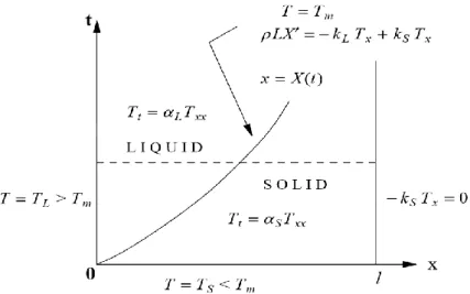
Let us now consider a two phase Stefan problem as presented by Alexiades and Solomon (1993):

Physical problem: Melting of a semi-infinite slab, 0≤x≤∞, initially solid at a uniform

temperature Ts≤Tm, by imposing a constant temperature TL>Tm on the face x=0.

Thermophysical parameters ρ, cL, cs, kL, kS, L, 𝛼𝑠= 𝑘_𝑠 𝜌𝑐𝑠, 𝛼𝐿=

𝑘_𝐿

𝜌𝑐𝐿, all constant. The

schematic representation of this problem can be observed in figure 1.2.

Figure 2.2. Two phase Stefan problem, Alexiades et al 1993

Physically, the above problem represents a tube filled with a PCM - Phase Change Material, being one of the phases exposed to a heat source, while the length of the tube is so high that the melting front cannot reach the other phase during the experiment.

9

Table 2.1. Overview of the most common assumptions on the Stefan problem, Alexiades et al 1993 Physical factors involved in phase change

processes

Simplifying assumptions for the Stefan

problem. Remarks on the assumptions

1.Heat and mass transfer by conduction,

convection, radiation with possible gravitational, elastic, chemical, and electromagnetic effects

Heat transfer isotropically by conduction only, all other effects assumed negligible.

Most common case. Very reasonable for pure materials, small container, moderate temperature gradients.

2.Release and absorption of latent heat Latent heat is constant; it is released or

absorbed at the phase-change temperature. Very reasonable and consistent with the rest of the assumptions.

3.Variation of phase-change temperature Phase-change temperature is a fixed known

temperature, a property of the material. Most common case, consistent with other assumptions.

4.Nucleation difficulties, supercooling effects Assume not present. Reasonable in many situations.

5.Interface thickness and structure

Assume locally planar and sharp (a surface separating the phases) at the phase change temperature.

Reasonable for many pure materials (no internal heating present).

6.Surface tension and curvature effects at the

interface Assume insignificant. Reasonable and consistent with other assumptions.

7.Variation of thermophysical properties Assume constant in each phase, for simplicity

(cL≠cS, kL≠kS).

An assumption of convenience only. Reasonable for most materials under moderate temperature variations. The significant aspect is their discontinuity across the interface, which is allowed.

8.Density changes Assume constant (ρL=ρS).

Necessary assumption to avoid movement of the material. Possibly the most unreasonable of the assumptions.

10

As said before the objective is to discover the temperature distribution T(x,t) as well as the interface location X(t), accordingly to the following conditions:

Heat equation in the melting region:

𝑇𝑡= 𝛼𝐿𝑇𝑥𝑥, 0 < 𝑥 < 𝑋(𝑡), 𝑡 > 0 (2.1a)

Heat equation in the solid region

𝑇𝑡= 𝛼𝑠𝑇𝑥𝑥, 𝑋(𝑡) < 𝑥, 𝑡 > 0 (2.1b) Interface temperature 𝑇(𝑋(𝑡), 𝑡) = 𝑇𝑚, 𝑡 > 0 (2.1c) Stefan’s condition 𝜌𝐿𝑋′_{(𝑡) = −𝑘} 𝐿𝑇𝑥(𝑋(𝑡)−, 𝑡) + 𝑘𝑆𝑇𝑥(𝑋(𝑡)+, 𝑡), 𝑡 > 0 (2.1d)

There is a convention where the solid corresponds to the negative sign, while the liquid is given by the positive one.

The right hand side of equation 2.1d represents a change in the heat flux qL-qS in x=X(t). The

notation 𝑇𝑥(𝑋(𝑡)±, 𝑡) is used to remember these values are the limit of 𝑇𝑥(𝑥, 𝑡), when 𝑥 →

𝑋(𝑡)±_.

Initial conditions

𝑇(𝑥, 0) = 𝑇𝑆< 𝑇𝑚 , 𝑥 > 0, 𝑋(0) = 0 (2.1e)

Boundary conditions

𝑇(0, 𝑡) = 𝑇𝐿> 𝑇𝑚, lim𝑥→∞𝑇(𝑥, 𝑡) = 𝑇𝑆, 𝑡 > 0 (2.1f)

2.3.1. The Neumann solution

In this section will be discussed a method for the solvability of the Stefan problem. Let us begin with the introduction of the similarity variable:

𝜉 = 𝑥

√𝑡 (2.2)

Therefore, we are seeking a solution in the form of:

𝑇(𝑥, 𝑡) = 𝐹(𝜉) (2.3)

The function 𝐹(𝜉) is unknown. On the other hand, the location of the interface is proportional to √𝑡 . As a result there is a proportional constant A which must be found.

11

Now, replacing in equation 2.1 and integrating, it is possible to obtain the new equation 2.5, with B and C as constants.

𝐹(𝜉) = 𝐵 ∫ 𝑒 𝑆2 4𝛼𝐿 𝜉 0 𝑑𝑠 + 𝐶 = 𝐵√𝜋𝛼𝐿erf ( 𝜉 2√𝛼𝐿) + 𝐶 (2.5)

At this point, it is of good practice to reformulate the initial problem, to accommodate the similarity solution. As such the objective is to discover the solution of 𝑋(𝑡) = 2𝜆√𝛼𝐿𝑡, for

𝑇(𝑥, 𝑡) = 𝐹𝐿(𝜉), in the liquid phase and for 𝑇(𝑥, 𝑡) = 𝐹𝑆(𝜉) in the solid one, being λ an unknown

constant and FL and FS unknown functions of the similarity variable (𝜉). Then the new

formulation is given by: Interface location

𝑋(𝑡) = 2𝜆√𝛼𝐿𝑡, 𝑡 > 0 (2.6a)

Temperature in the liquid phase 0 < 𝑥 < 𝑋(𝑡), 𝑡 > 0 𝑇(𝑥, 𝑡) = 𝑇𝐿− (𝑇𝐿− 𝑇𝑚)

erf( 𝑥

2√𝑡𝛼𝐿)

erf (𝜆) (2.6b)

Temperature in the solid phase 𝑥 > 𝑋(𝑡), 𝑡 > 0 𝑇(𝑥, 𝑡) = 𝑇𝑆+ (𝑇𝑚− 𝑇𝑠) erf( 𝑥 2√𝑡𝛼𝑆) erf(𝜆√𝛼𝐿 𝛼𝑆) (2.6c)

Solution of the transcendental equation (λ)

𝑆𝑡𝐿 exp (𝜆2_{)erf (𝜆)}− 𝑆𝑡𝑆 𝜈exp (𝜈2_𝜆2_{)𝑒𝑟𝑓𝑐(𝜈𝜆)}= 𝜆√𝜋 (2.6d) with: 𝑆𝑡𝐿= 𝑐𝐿(𝑇𝐿−𝑇𝑚) 𝐿 , 𝑆𝑡𝑆= 𝑐𝐿(𝑇𝑚−𝑇𝑆) 𝐿 , 𝜈 = √ 𝛼𝐿 𝛼_𝑆 (2.7)

The factors 𝑆𝑡𝐿 and 𝑆𝑡𝑆 present in equation 2.7 represent the Stefan number for a melting and

freezing process, which notes the quotient between sensible and latent heat. The sensible heat is described as the one that is related to the temperature increasing. Therefore:

𝑠𝑒𝑛𝑠𝑖𝑏𝑙𝑒 ℎ𝑒𝑎𝑡 = ∫ 𝐶(𝑇)𝑑𝑇_𝑇𝑇

𝑚 (2.8)

The objective of the Stefan number is to determine if a given method is appropriate to analyze the phase change process. While high Stefan numbers mean the process will be of pure conduction, low magnitude numbers state it will be dominated by the phase change.

12

Another notable aspect is related with the enthalpy. At T=Tm, the enthalpy has a jump of

magnitude L. Any region in which T=Tm and 0<e<L is referred as a mushy zone. Accordingly to

the number 5 of table 2.1 the interface’s thickness will be equal to 0.

The transcendental equation has only one solution for λ >0, which means the similarity solution is unique for 𝑆𝑡𝐿> 0, 𝑆𝑡𝑆≥ 0, , 𝜈 >0.

For a two phase freezing process, the Neumann solution is obtained changing the subscripts L for S and the latent heat from L to –L.

The interface is the frontier that divides the solid and liquid regions, meaning there is a need for a frontier condition for each phase in order to achieve a solution. It is given the temperature must be continuous and at Tm follows an isotherm, translated into:

lim𝑥⃗→𝑖𝑛𝑡𝑒𝑟𝑓𝑎𝑐𝑒 𝑥⃗ ∈ 𝑙𝑖𝑞𝑢𝑖𝑑 𝑇(𝑥⃗, 𝑡) = 𝑇𝑚 (2.9) lim𝑥⃗→𝑖𝑛𝑡𝑒𝑟𝑓𝑎𝑐𝑒 𝑥⃗ ∈ 𝑠𝑜𝑙𝑖𝑑 𝑇(𝑥⃗, 𝑡) = 𝑇𝑚 (2.10)

If the interface location was known, there would be a necessary conditions to determine the temperature in each phase.

Regarding the Stefan condition, introduced in this subsection, it denotes the latent heat released due to movement of the interface equals the flux of heat per unit time. As a result, the Stefan condition represents a heat balance across the interface.

In other words, the Stefan condition shows the latent heat rate change 𝜌𝐿𝑋′_{(𝑡) equals the}

heat that jumps across the interface. In particular, the heat flux can be continuous if and only if L=0 or the interface does not move. When discussing a cylinder or a sphere the characteristic length is the radius.

In a final note, the functions T(x,t) and X(t) constitute a solution to the Stefan problem up to a time t*, if the functions’ derivatives of every order, which appear in the problem formulation are continuous and satisfy the problem conditions. The time t* designates the time up to which the solution is desired.

There are methods called front tracking schemes, which try to find the interface’s location through the Stefan number.

2.4. Density considerations

Changes in density induce movement of the material and further complicate the modeling of phase change processes. For most materials ρL<ρS, meaning they expand upon melting, which

13

There are two different kinds of density change of particular importance in phase change processes. The first one is the already mentioned difference between phases, the other being the density variation with temperature. A liquid density diminishes with the increasing temperature and as a consequence, much hotter the liquid is, more volume will occupy. In the presence of gravity, a temperature gradient induces a flux due to buoyancy called natural convection, modeled by the Rayleigh number.

Let us consider the case of a shrinking in a closed container with ρL<ρS. The formatting solid

occupies less volume as a consequence of the relation between densities. Therefore the container gets under pressurized. From this point, two consequences were theorized: either the container or the PCM will break. If the container is strong enough, voids are formed, fulfilled with the material’s vapor. The place where they form depends on the magnitude of the adhesion forces: wall-liquid, wall-solid, liquid-solid or within the liquid or the solid. Usually the weakest forces are registered between the wall and the PCM.

There is also the possibility of microbubbles of pre-existent air be trapped within the liquid. These bubbles will fluctuate to the top- buoyancy- even in zero gravity- Marangoni flow- due to the surface tensions. Marangoni result from either temperature of chemical concentration gradients at the interface.

The modulation of these complicated phenomenon is approached in the context of energy storage in space systems, with resource to the Navier-Stokes equations and thermodynamic knowledge of the interface.

2.5. Approximations

The most important characteristic of the explicit solutions in phase change problems is that they provide real insight of how the different parameters at study interact with the factors of interest to us.

The number of problems with explicit solution is extremely low and in most cases, they don’t have relevance in real life situations. Explicit solutions exist to problems with constant parameters in each phase and imposed temperature, which leaves imposed flux out of the picture.

As a result, there is a need to use approximations: analytical and numerical. The downside arises from the fact that there is no way of verify the validity of the simplifications and there are no error approximations to the mathematical ones. On the other hand, there are problems that remain even when a system is reduced to its most basic form. Examples can be found in Temos et al (1996), regarding mass transfer. There, they pay a closer look to mass transfer in initially insulated droplets and conclude that even for such a system there are several problems as:

14

I. Interface contamination, which will reduce the mass transfer, when compared with a pure system;

II. Interface instability, with the consequence of pressure gradients that will increase the mass flow (Marangoni)

III. Hydrodynamic changes within the droplet, due to stagnation in oscillation, which influences the boundary layer and vortex shedding.

It has become clear by previous studies, the mass transfer is deeply affected by hydrodynamic factors. However a detailed explanation of the droplet dynamics is only available for special cases, but generalizations can be built with the drag coefficient graphic as seen in Temos et

al (1996).

2.5.1. Analytical approximations

The validity of an analytical approximation is made from comparison with the results of other independently validated method. These provide qualitative and magnitude information, instead of just quantitative.

Now the main analytical approximations will be introduced, as well as their most relevant aspects.

2.5.1.1. Quasistationary approximation (Alexiades et al 1993)

I. Simplify the heat equation to its steady state

II. One phase method (Cartesian, cylindrical or spherical coordinates)

III. The sensible heat is negligible in comparison to the latent heat (Stefan number) IV. Overestimate the interface location

V. Simple for determination of the feasibility and estimate sizing of the problem

VI. First cut answers, which through any other way would require costly computational estimation.

VII. Low accuracy

2.5.1.2. Megerlin method (Alexiades et al 1993)

I. Assume parabolic temperature profile II. May be difficult to use

III. If the boundary data are not constant, there won’t be an explicit solution IV. Solvability with convective boundary conditions

V. It can violate the conservation of energy, since this equation is only satisfied at the boundary

15

2.5.1.3. Heat balance integral method (Sethian et al 1993 & Lunardini 1981)

I. Assume parabolic temperature profile II. May be difficult to use

III. Seeks to satisfy a global heat balance explicitly

IV. Given the impossibility of error determination, the choice between this method and the Megerlin method becomes a matter of personal preference

2.5.1.4. Perturbation method (Alexiades et al 1993)

I. Uses mathematical expansion in series to reduce a larger problem into simple ones with explicit solution

II. Represents a high order correction of the quasistacionary approximation III. Convenient and efficient dimensionless formulation

IV. Interface location is fixed in space

2.5.2. Numerical approximations (Caginalp et al 1991 and Fix et al 1988)

There are several aspects of numerical approximations common to all algorithms that are presented next:

I. Physical region approximated by a small number of control volumes

II. Idealized mathematical concepts like integrals and derivatives must be re-approximated by finite-differences methods

III. The most common numerical method for the simulation of phase change processes IV. High temperature gradients require the use of small control volumes and small

temperature gradients can be acquired by large control volumes

V. Control volumes are regions where local equilibrium is achieved in a time scale smaller than the time step

VI. Finite-differences result from control volume discretization

The numerical approximations may be divided into different paths, depending on the objectives of the work. Let us then define the mathematical work region.

The region M is divided into control volumes. To each sub region Vj is associated a node xj.

There is also a need to define ΔVj as the volume of Vj and Aij=Aji the common area of Vi e Vj.

16

Fully implicit scheme: 𝐸𝑗𝑛+1= 𝐸𝑗𝑛+

Δ𝑡𝑛

Δ𝑥_𝑗(𝑞𝑗−1/2 𝑛+1 _{− 𝑞}

𝑗+1/2𝑛+1 ), 𝑗 = 1, … , 𝑀, 𝑛 = 0,1, … (2.12)

The quotient between length and thermal conductivity is defined as thermal resistance, where the temperature drop ΔT is called thermal driving force:

𝑡ℎ𝑒𝑟𝑚𝑎𝑙 𝑟𝑒𝑠𝑖𝑠𝑡𝑒𝑛𝑐𝑒 =_{(𝑐𝑟𝑜𝑠𝑠𝑒𝑐𝑡𝑖𝑛𝑎𝑙 𝑎𝑟𝑒𝑎)∗(𝑐𝑜𝑛𝑑𝑢𝑐𝑡𝑖𝑣𝑖𝑡𝑦)}𝑙𝑒𝑛𝑔𝑡ℎ 𝑜𝑓 𝑟𝑒𝑠𝑖𝑠𝑡𝑎𝑛𝑐𝑒 𝑝𝑎𝑡ℎ (2.13)

The standard centered difference discretization of Txx is given by equation 2.14. For plain

heat conduction, as defined when we discussed the Stefan problem, the total energy is the sensible heat. Also, due to irregularities at the interface, the thermal conductivity is not a constant, but a function of the position.

𝐸𝑗𝑛+1= 𝐸𝑗𝑛+ 𝑘Δ𝑡𝑛

Δ𝑥2 ∗ (𝑇𝑗−1𝑛+𝜃− 2𝑇𝑗𝑛+𝜃+ 𝑇𝑗+1𝑛+𝜃) (2.14)

The discrete problem is then defined as: Initial values: 𝑇_𝑗0_{= 𝑇} 𝑖𝑛𝑖𝑡(𝑥𝑗), 𝑗 = 1, … , 𝑀 (2.15a) Boundary condition at x=0: 𝑞_1/2𝑛+𝜃_{= −}𝑇1𝑛+𝜃−𝑇∞𝑛+𝜃 1 ℎ+𝑅1₂ , 𝑅1/2= 1/2𝛥𝑥 𝑘1 (2.15b) Boundary condition at x=l: 𝑞_𝑀+1/2𝑛+𝜃 _{= 0 (2.15c)} Interior values: 𝑇𝑗𝑛+1= 𝑇𝑗𝑛+ Δ𝑡𝑛 𝜌𝑐_𝑗Δ𝑥_𝑗∗ (𝑞𝑗−1/2 𝑛+𝜃 _{− 𝑞} 𝑗+1/2𝑛+𝜃 ), 𝑗 = 1, … , 𝑀 (2.15d) Where: 𝑞𝑗−1/2𝑛+𝜃 = − 𝑇_𝑗𝑛+𝜃−𝑇_𝑗−1𝑛+𝜃 𝑅_𝑗−1/2 , with 𝑅𝑗−1/2= 1/2Δ𝑥𝑗−1 𝑘_𝑗−1 + 1/2Δ𝑥𝑗 𝑘_𝑗 , 𝑗 = 2, … , 𝑀 and 𝑇𝑛+𝜃_{= (1 − 𝜃)𝑇}𝑛_{+ 𝜃𝑇}𝑛+1 _(2.15e)

17

In this case, the discretization replaces a partial differential equation (𝑃𝐷𝐸[𝑢] = 0) by a finite-difference equation (𝐹𝐷𝐸[𝑢𝑗𝑛] = 0). A consistent finite-difference method for a well

posed problem is convergent if and only if is stable – Lax equivalence theorem. The local truncation error is given by:

𝑡𝑒𝑗𝑛≔ 𝐹𝐷𝐸[𝑢(𝑥𝑗, 𝑡𝑚)] (2.16)

The local discretization error is given by:

𝑑𝑒𝑗𝑛≔ 𝑈𝑗𝑛− 𝑢(𝑥𝑗, 𝑡𝑛) (2.17)

The simplicity and convenience of the explicit scheme is posed against the restraint necessity of the time step, in order to achieve numerical stability of the formulation.

The stability condition known as CFL-Courant-Friedrichs-Lewy is: Δ𝑡 ≤1

2 Δ𝑥2

𝛼 (2.18)

Errors are represented by Fourier series expansions and typical Fourier amplification factors are calculated.

A simple method to achieve stability is the “positive coefficient rule” fully described in Patankar et al 1980 and Anderson 1995, where 𝑇_𝑗𝑛+1 _{is written as a linear combination of its}

neighbors.

The CFL condition can be altered when facing different boundary conditions: Δ𝑇𝑛<

1 3

Δ𝑥_𝑚𝑖𝑛2

𝛼𝑚𝑎𝑥 (2.19) for imposed temperatures and convective conditions

Δ𝑇𝑛< 1 2

Δ𝑥_𝑚𝑖𝑛2

𝛼𝑚𝑎𝑥 (2.20) for imposed flux conditions

There is a recommendation in the literature to use the fully implicit discretization to boundary nodes.

18

2.5.2.1. Enthalpy formulation (Smith 1981)

The main features of this formulation are presented below:

I. Bypasses the explicit track of the interface. The Stefan condition is met automatically as a natural boundary condition

II. The enthalpy formulation (also referred to in literature as weak formulation) is very similar to the method used in gas dynamics to chocking.

III. The enthalpy method discretized by finite differences is the most versatile, convenient and the simplest to program in phase change problems in 1,2 and 3D. (However it does not solve every problem)

IV. The volume occupied with the PCM is divided in an infinite number of control volumes Vj and then, energy conservation is applied, meaning a discrete energy balance is

used to update the enthalpy at every control volume

V. The phases are determined just by the enthalpy, with no mention to the interface location - volume tracking scheme (Sullivan et al 1987)

The discrete problem is defined as: Initial values: 𝑇_𝑗0_{= 𝑇} 𝑖𝑛𝑖𝑡(𝑥𝑗), 𝑗 = 1, … , 𝑀 (2.21a) Boundary condition at x=0: 𝑞1/2𝑛+𝜃= − 𝑇₁𝑛+𝜃−𝑇∞𝑛+𝜃 1 ℎ+𝑅1₂ , 𝑅1/2= 1/2Δ𝑥 𝑘1 (2.21b) Boundary condition at x=1: 𝑞𝑀+1/2𝑛+𝜃 = 0 (2.21c) Interior values: 𝐸_𝑗𝑛+1_{= 𝐸} 𝑗𝑛+ Δ𝑡𝑛 Δ𝑡𝑗[𝑞𝑗−1₂ 𝑛+𝜃_{− 𝑞} 𝑗+1 2 𝑛+𝜃_{] , 𝑗 = 1, … , 𝑀 (2.21d)} With: 𝑞𝑗−1/2𝑛+𝜃 = − 𝑇_𝑗𝑛+𝜃−𝑇_𝑗−1𝑛+𝜃 𝑅_𝑗−1/2 , com 𝑅𝑗−1/2= 1/2Δ𝑥𝑗−1 𝑘_𝑗−1 + 1/2𝑥𝑗 𝑘_𝑗 , 𝑗 = 2, … , 𝑀 (2.21e) And 𝑓(𝑥) = { 𝑇𝑚+ 𝐸_𝑗𝑛 𝜌𝑐𝑆, 𝐸𝑗 𝑛_{≤ 0 (𝑠𝑜𝑙𝑖𝑑)} 𝑇𝑚, 0 < 𝐸𝑗𝑛≤ 𝜌𝐿 (𝑖𝑛𝑡𝑒𝑟𝑓𝑎𝑐𝑒) 𝑇𝑚+ 𝐸_𝑗𝑛−𝜌𝐿 𝜌𝑐𝐿 , 𝐸𝑗 𝑛_{≥ 𝜌𝐿 (𝑙𝑖𝑞𝑢𝑖𝑑)} (2.22)

19

The algorithm presented previously has the following methodology: knowing the temperature and the phase of each control volume, the resistances are computed and the fluxes, which are then used to update the enthalpies that produce new temperatures and phase states. In situations where the time step must be small for physical reasons, the explicit scheme may turn out to be as efficient as the implicit one.

The implicit scheme is more advantageous for slow phase change processes than for faster ones.

Explicit schemes have inherent limitations in relation to the time step, imposed by the stability conditions. On the other hand, even fully implicit schemes must have restrictions regarding the time step, to attain precision. The loss of precision occurs when the following is not respected:

|𝑋′_{|Δ𝑡 ≤ Δ𝑥 (2.23)}

The faster the melting process is, the lower will the time step be, in order to have acceptable precision. Therefore the implicit scheme is less advantageous. The explicit scheme is mainly used to exploratory studies.

The enthalpy method is flexible enough to allow the sample (wall + PCM) to be treated as a unique region, but with different thermophysical properties to both phases.

The basic limitation of the classical formulation, as seen before, lies with the fact the interface must be assumed a sharp interface. This is particularly problematic when discussing cyclic melting/freezing problems, where several interfaces are likely to appear. In this case, it would be necessary to know the interfaces structures a priori.

Even with numerical approximations there are problems in which the mathematical models are not totally adequate like biphasic flows. As a result, there is the need to use experimental data to validate the model. On the other hand it is necessary to develop the models so they approximate more the physical processes.

21

3. Mathematical models

3.1. Introduction

In this chapter first a mathematical model for the calculation of heat and mass transfer on a system of free falling drops is described. Then a four phase freezing model with supercooling is introduced. This chapter concludes by describing the initial conditions to be used in the numerical simulations, as well as the computational domain configuration.

3.2. Heat and mass transfer on a system of free falling drops

This section describes a model for the calculation of heat and mass transfer coefficients for a system of free falling drops in moist air conditions. It starts by presenting and explaining the processes behind a single drop modulation and then it evolves until the procedure for the calculations of a system of drops is presented.

According to Hindmarsh et al (2003), the techniques used for the analysis of water droplets can be divided into two categories: free flight, which is the current case and levitation. Levitation is further divided into intrusive and non-intrusive techniques, exemplified in figure 3.1.

Figure 3.1. Techniques for the study of single drops

In free flight, the present case, the drops fall through the air and the different variables are measured by observation or by catching the drops at various heights. On the other hand, on levitation techniques the drops remain stationary, while the air flows past them.

Let us consider a jet discharged from a nozzle, in particular onwards from the point where it breaks into single individual drops due to inertial and aerodynamic forces. In order to determine the rate of heat and mass transfer from the drops, their velocity needs to be calculated. While along the horizontal axis, in the breaking point of the jet, the velocity’s

Techniques for the study of single drops

Levitation

Intrusive Non-intrusive

22

component is negligible, the same cannot be said of its vertical component. Here it is assumed the drops equal their terminal velocity which will be used later on the Reynolds’ number calculation.

The movement equation of a drop of d diameter, accordingly to Lapple and Sheperd (1940) is given by: 𝑑𝑈⃗⃗⃗ 𝑑𝜏

+

(

) |𝑈

⃗⃗⃗|𝑈⃗⃗⃗ + 𝑔⃗ (

− 1) = 0

At the terminal velocity in yy direction, with 𝑑𝑈⃗⃗⃗

𝑑𝜏=0, Uy can be calculated with:

𝑈𝑦= √

4𝑑𝑔(𝜌_𝑤−𝜌_𝑎)

3𝜌𝑎𝐶𝐷 (3.2)

For liquid droplets, the Reynols number can be evaluated from:

𝐶𝐷 = 24 𝑅𝑒+ 6 1+√𝑅𝑒+ 0.27, 1 < 𝑅𝑒 ≤ 1000 (3.3 a) 𝐶𝐷=0.6649 − 0.2712𝐸−3𝑅𝑒 + 1.22𝐸−7𝑅𝑒2− 10.919𝐸−12𝑅𝑒3, &3600 ≥ 𝑅𝑒 ≥ 1000 (3.3 b)

This model allows for the calculation of the heat and mass transfer maximum rates, however it does not take into account changes in temperature and air humidity as the drop falls. The next parameter to take into account is the approach to be used in the calculation of the transfer rate of mass and heat: complete mixing model or non-mixing model. For complete mixing it is necessary to assume the drop’s internal motion to be so powerful in order to reach complete mixing. In this case the temperature profile is planar and the only place where heat and mass transfer occur is at the drop’s surface. On the other hand considering there’s no mixing within the drop leads to the reduction of the energy equation to a problem in transient regime. The heat flow achieved if the first option is used is superior to the flow obtained through the second.

Strub et al, 2003 studied the freezing of a single water droplet, in particular the importance of evaporation on the overall freezing process and the impact of drops’ size and velocity and air’s humidity ratio and temperature on the crystallization phase.

23

The left hand side of equation 3.4 represents the rate of energy change as the drop falls. The right hand side terms represent the transport of energy by convection, evaporation and radiation, respectively. The heat and mass transfer coefficients are constant.

The radiation may be determined with the introduction of the heat radiation term: ℎ𝑟= 𝜎𝑒(𝑇𝑤2+ 𝑇∞2)(𝑇𝑤+ 𝑇∞) (3.5)

The next step is to express the evaporation in term of temperature. Being the humidity saturation rate a function of temperature, a parabolic curve with the temperature as an independent variable may be used:

𝑊𝑠= 𝑎𝑇𝑤2+ 𝑏𝑇𝑤+ 𝑐 (3.6)

Now passing from a single drop to a system, a water column with the shape of a cylinder will be considered as a representative model. An overall representation of the variables involved is presented in figure 3.2.

Figure 3.2. Heat and mass balance of a column of air in a differential element

Cold air Tgi, Wi, vg Water Twi Water

ΔT

24

Introducing the balance equation, from figure 3.2 as:

𝑚𝑎𝑑ℎ = −[𝑚𝑤− 𝑚𝑎(𝑊 + 𝑑𝑊 − 𝑊𝑖)]𝑑ℎ𝑓+ 𝑚𝑎ℎ𝑓𝑑𝑊 (3.7)

It can be simplified to:

𝑚𝑎𝑑ℎ = −𝑚𝑤𝑑ℎ𝑓+ 𝑚𝑎ℎ𝑓𝑑𝑊 (3.8)

The model starts by assuming a set of adequate initial conditions for the beginning of the calculation procedures. At this point values for the initial air and water temperatures, humidity ratio, drop diameter, air column height, flow ratio, air velocity and drop diameter are set.

A differential control volume is established to divide the water column in smaller portions in which the calculation procedure will be repeated until the bottom of the column is reached. This allows for a better accuracy of the results. For instance if a greater accuracy is desired, smaller step sizes, meaning a greater number of control volumes can be used.

The change of energy in the water, within the control volume is due to the heat and mass convection from the drops:

−𝑚𝑤𝑑ℎ𝑓 = ℎ𝑐𝐴𝑣𝑑𝑉(𝑇𝑤− 𝑇𝑎) + 𝜌𝑎ℎ𝑑𝐴𝑣𝑑𝑉(𝑊𝑠− 𝑊)ℎ𝑓𝑔 (3.9)

The left hand side of the above equation represents the energy change in the water, while the right hand side represents heat transfer due to convection and evaporation.

The change in the concentration of water vapor must equal the mass transfer in drops, or when WS and W are the humidity ratios.

The heat and mass transfer coefficients calculated from the Ranz-Marshall relations are presented here in equations 3.10 and 3.11, according to Ranz et al, 1952:

𝑁𝑢 =ℎ0𝑑 𝐾𝑔 = 2 + 0.6𝑅𝑒𝑑 1 2 ⁄ 𝑃𝑟_𝑑1⁄3 _(3.10) 𝑆ℎ = ℎ𝑚𝑑 𝐷𝑣𝑔 = 2 + 0.6𝑅𝑒𝑑 1 2 ⁄ 𝑆𝑐_𝑑1⁄3 _(3.11)

25

Tang et al 1993 presented a document, in which they show a one-dimensional numerical model for liquid and solid drops in free-fall. In this document, a review of previews studies around the Ranz-Marshall relations is presented.

The Sherwood number for mass transfer is analogous to the Nusselt number for convective heat transfer.

The Schmidt number as the same relation between mass and momentum as the Prandtl between momentum and heat Hines and Maddox (1985).

In order to reach the desired coefficients, the Reynolds, Prandtl and Schmidt numbers are calculated according to equations 3.12 to 3.14.

𝑅𝑒 =𝑣𝑟.𝑑 𝜈 (3.12) 𝑃𝑟 =𝜈 𝛼 (3.13) 𝑆𝑐 =𝜈 𝐷 (3.14)

The thermal diffusivity, viscous diffusivity, mass diffusivity and thermal conductivity are calculated according to Ashrae, 1977:

α = 1 57736−585.78T_a (3.15) ν = 1 80711.7−766.15Ta (3.16) D = 2.227 × 10−5(Ta+273 273 ) 1.81 (3.17) k = 0.024577 + 9.027 × 10−5_T a (3.18)

Now let us determine The Lewis number, which relates the convective heat transfer with the convective mass transfer to the water:

𝐿𝑒 = ℎ𝑐 𝜌𝑎𝐶𝑝,𝑎ℎ𝑑≅ ( 𝛼 𝐷) 2/3 (3.19)

With the Lewis’ number introduction, equation 3.9 is transformed into:

−𝑚𝑤𝑑ℎ𝑓= 𝜌𝑎ℎ𝑑𝐴𝑉𝑑𝑉[𝐿𝑒𝐶𝑝,𝑎(𝑇𝑤− 𝑇𝑎) + (𝑊𝑠− 𝑊)ℎ𝑓𝑔] (3.20)

26

ℎ = 𝐶𝑝,𝑎𝑇𝑎+ 2501𝑊 (3.21)

The next step is to calculate the variation in the humidity ratio across a control volume which is given by:

𝑚𝑎𝑑𝑊 = 𝜌𝑎ℎ𝑑𝐴𝑣𝑑𝑉(𝑊𝑠− 𝑊) (3.22)

And the saturation humidity:

Ws= 0.003894e0.094442Tw (3.23) Finally: 𝑑ℎ 𝑑𝑊= 𝐿𝑒 (ℎ𝑠−ℎ) (𝑊_𝑆−𝑊)+ (ℎ𝑔− 2501𝐿𝑒) (3.24)

Equation 3.24 represents the changes of state, in enthalpy variation as the drop goes through the air column, making possible for the calculation of the temperature variation:

𝛥𝑇𝑊= − 𝑚_𝑎

𝑚𝑤𝐶𝑝(𝛥ℎ − ℎ𝑓𝛥𝑊) (3.25)

Then the humidity ratio, the enthalpy of the air stream and the temperature of the water are incremented for the determination of the conditions on the other side of a control volume until the bottom of the column is reached. This value can be confirmed through a balance to the entire water column, represented by:

𝑚𝑎ℎ𝑎𝑖+ 𝑚𝑤ℎ𝑓,𝑖 = 𝑚𝑎ℎ𝑎𝑜+ [𝑚𝑤− 𝑚𝑎(𝑊𝑜− 𝑊𝑖)]ℎ𝑓,𝑜 (3.26)

If the air temperature is known, the mean mass transfer coefficient, hdAV, is known, the

volume of air is: 𝑉 = 𝑚𝑎 ℎ𝑑𝐴𝑉∫ 𝑑𝑊 𝑊𝑠−𝑊 𝑊0 𝑊_𝑖 (3.27)

This model for a system of drops allows, as for the single drop case, for the calculation of maximum heat and mass transfer rates and takes into account changes in temperature and humidity ratio as the drop falls. However as studied by Yao et al 1976, vibrations and deformations of the falling drops have an impact on heat and mass transfer coefficients’ values. The model here described in section 3.1. is summarized and presented in graphic form in figure 3.3

27

Figure 3.3. Flowchart for the calculation of the rate of cooling of a system of drops in free fall

Since both the non-mixing and the complete mixing model represent extreme situations, a correction factor which accounts for such distortions and vibrations, giving a solution in closer agreement with the experimental data was developed and is here present in equation 3.28.

𝑔 = 25 (𝑥

𝑑) −0.7

(3.28)

Start

Initial gas temperature

Initial humidity ratio

Gas velocity

Initial water temperature

Drop diameter

Initial flow ratio

Water column height

Humidity ratio variation within the control volume

Water vapor enthalpy variation within the control volume

Water temperature variation within the control volume

Is the bottom of the water

column reached?

Water temperature variation

End

No

28

The correction factor developed approximates the complete mixing model with the experimental data for drops of water from 3 up to 6 mm in diameter for a ratio of x/d up to 600. Then, it is used along with the Ranz-Marshall relations already presented in equations 3.10 and 3.11, for a more realistic calculation of the heat and mass transfer coefficients.

Nu = 2 + 15Re_d1⁄2_Pr d 1 3 ⁄ (x d) −0.7 (3.29) Sh = 2 + 15Re_d1⁄2_Sc d 1 3 ⁄ (x d) −0.7 (3.30)

3.3. Four phase freezing with supercooling

Previous studies, Hallet (1964), have devoted themselves to the search of a relation between the ice crystal structure, the rate of supercooling and the nucleation method. Various methods were tried over the years, such as polarized light in ice tunnels, at known conditions of size distribution and supercooling. From these researches comes an expression to the calculation of the water to ice ratio:

∫ 𝜎𝑇𝑑𝑇

𝐿𝑇

Δ𝑇

0 (3.31)

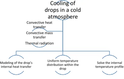
For the development of a numerical model, each phase of the freezing process needs to be described individually. The prediction of the phase change temperature of each phase was achieved through the droplet’s internal energy and heat losses to the environment. A scheme of the physical processes and main assumptions of the numerical model is presented in figure 3.4.

Figure 3.4. Main factors of the numerical solution

Cooling of

drops in a cold

atmosphere

Modeling of the drop’s internal heat transfer

Uniform temperature distribution within the

drop

Solve the internal temperature profile Convective heat transfer Convective mass transfer Thermal radiation

29

An energy balance is enough for the modeling of the freezing stage, through the external heat transfer and the amount of latent heat to be removed for the complete freezing of the mass of water within the drop.

Figure 3.5. Generic representation of a four phase freezing process, Hindmarsh et al 2003 and Tanner et al 2011

This physical representation of a phase change process is composed by a supercooling period, where the temperature drops below Tf, followed by a recalescence stage, then a crystal

growth phase and for last a cooling stage. Let us then discuss in a more detailed manner what physical processes are involved in each stage accordingly to figure 3.5.

I. Supercooling: the liquid drop is frozen from its initial temperature to the nucleation temperature (Tn), that lies below the equilibrium freezing temperature (Tf)

II. Recalescence: the supercooling stage induces a rapid kinetic growth of the crystal, with the release of latent heat, which results in a temperature increase until it reaches the equilibrium temperature

III. Solidification or freezing: the crystal growth happens at a constant equilibrium freezing temperature, until the droplet is completely solidified

IV. Cooling or tempering: the solidified drop freezes until it reaches the ambient temperature

The cooling of the solid particles in stages I and IV is determined by the energy exchange between the particles themselves and the environment. The internal temperature profile can be solved through a description between the transient heat transfer equations, with the help of appropriate boundary conditions. The heat transfer in stage III is a Stefan typical problem, which as described in the introductory chapter, consists in determining the temperature distribution and the interface’s location.

30

Translating the text into mathematical language, it is known for a uniform temperature distribution the rate of temperature change is given by:

𝜌𝑑𝑉𝑑𝐶𝑝𝑑 𝑑𝑇𝑑

𝑑𝑡 = −𝑆𝑑(𝑞ℎ+ 𝑞𝑚+ 𝑞𝑟) (3.32)

Where 𝑞ℎ is set accordingly to Newton’s cooling law: 𝑞ℎ= ℎ0(𝑇𝑑− 𝑇𝑔) and 𝑞𝑚 from:

𝑞𝑚= 𝐿ℎ𝑚(𝜌𝑣− 𝜌𝑔) (3.33)

The convective coefficients once again arise from the Ranz-Marshall relations already explained through equations 3.10 and 3.11.

For last, the thermal flux due to radiation is achieved with the Stefan-Boltzmann fourth power law: 𝑞𝑟= 𝜀𝜎(𝑇𝑑4− 𝑇𝑔4) (3.34)

As seen through figure 3.6, a drop with initial supercooling, after the nucleation stage suffers a temperature increase until it reaches Tf. During this stage, which is recalescence, there is a

percentage of volume that solidifies - Vf.

𝑉𝑓= 𝑉𝑑

𝜌𝑑𝐶𝑝𝑑(𝑇𝑓𝑇𝑛)

𝜌𝑠𝐿𝑓 (3.35)

Since the gas temperature at the surface is usually different from the mean value, it is possible to account this discrepancy with the correction of two thirds the mean temperature:

𝑇 =𝑇𝑔+2𝑇𝑑

3 (3.36)

The dimensionless groups- the Reynolds, Prandtl and Schmidt numbers – depend on the properties of the gas (µg, Kg and Dvg),, which in turn depend on the temperature of the

surrounding gas. In order to accommodate these variations, it is possible to make use of the Sutherland relations: µ𝑔(𝑇) = 𝐴₁∗𝑇1.5 𝑇𝐴2 (3.37) 𝐾𝑔= 𝐾1∗𝑇1.5 𝑇∗𝐾2 (3.38) With: