Margarida Maria Correia Alves Lopes
Mestre em Clima e Ambiente Atmosférico
Ultrafine Particle Levels Monitored at
Different Transport Modes in Lisbon
Dissertation for obtainment of Doctor degree in
Environment and Sustainability
Advisor: Francisco Manuel Freire Cardoso Ferreira, PhD, Associate Professor, FCT/UNL
Co-Advisor: Célia Marina Pedroso Gouveia, PhD, Assistant Professor, IDL-FCUL
Presidente: Arguente(s):
Vogais:
Prof. Doutor António Nóbrega de Sousa Câmara Prof. Doutor Julio Lumbreras
Prof. Doutora Margarida Maria Correia Marques Prof. Doutor António Nóbrega de Sousa Câmara Prof. Doutor Francisco Manuel Freire Cardoso Ferreira Prof. Doutor Pedro Manuel da Hora Santos Coelho
Ultrafine Particle Levels Monitored at Different Transport Modes in Lisbon Copyright © Margarida Maria Correia Alves Lopes,
Faculdade de Ciências e Tecnologia da Universidade Nova de Lisboa, Universidade Nova de Lisboa. A Faculdade de Ciências e Tecnologia e a Universidade Nova de Lisboa têm o direito, perpétuo e sem limites geográficos, de arquivar e publicar esta dissertação através de exemplares impressos reproduzidos em papel ou de forma digital, ou por qualquer outro meio conhecido ou que venha a ser inventado, e de a divulgar através de repositórios científicos e de admitir a sua cópia e distribuição com objectivos educacionais ou de investigação, não comerciais, desde que seja dado crédito ao autor e editor.
Acknowledgments
This work started late in 2010. After many “ups and downs”, with a forced interruption of four years, it finally came to a conclusion. During these past eight years, there are many ones whom I’m deeply thankful, both in personal and professional levels. These lines won’t be enough to pay them my appreciation… still, I will do my best.
The first one I would like to thank is my supervisor, Prof. Francisco Ferreira. Thank you for the opportunity, for the precious guidance, for helping me through scientific research, for the freedom you gave me to find my own path and all the support to accomplish the work which make this thesis possible. Thank you for your infinite patience and contributions during the thesis writing stage, from its structure definition to contents discussion, and finally its proof reading Thank you for helping me through all difficult moments and facing all the adversities without losing hope. A very special thanks to my co-supervisor, Prof. Célia Gouveia. Your complementary knowledge, perspectives, objectivity and insightful comments allowed me to widen my research and enrich this work.
Secondly, I want to thank the Air Quality research group in the FCT-NOVA, for their friendship, for all the help and for being always there for me throughout this work and Ana Russo, from Instituto Dom Luiz, Faculty of Sciences of the University of Lisbon. Joana Monjardino, a precious co-author in my first paper, thank you for all the fresh viewings, perspectives, advices and precious guidance throughout my first scientific pear reviewed paper; Ana Russo, was a crucial co-author in both my scientific pear reviewed papers. Thank you so much for helping me with writing, analysis, review and corrections and answers to reviewers. Paulo Pereira and Sofia Teixeira, for the support and for being in the field helping me collecting traffic data; Luísa Mendes for the support on getting meteorological data and Hugo Tente, for some fresh ideas and perspectives.
Thank you, Helena Pandamo and Sandra Ferreira, for all the patience, competence and availability to solve all the administrative issues that came along this journey.
A very special thanks to my daughter, to whom I dedicate this work. Thank you so much for being such a grown up, independent and comprehensive person, now a 13 years old young “woman”. I will try to make it up for you over the coming years for all the time together we had to abdicate during this task. This is also your work and I hope it can make you proud. Thank you! My grand-mother, Hermínia Correia, wherever you are… you were a force of Nature and I always took you as an example and a life guidance. Wherever you are, I am sure you are feeling very proud and I am truly thankful for the privilege of learning from you and have you as my model guide. My mother and my father for the all support. My mother suffered as much as I did during this task and kept me confidant throughout this job; my father… well, I learnt from him that “it is only impossible until it is done” and he never doubt I would accomplish this goal. My family’s care and love were, are and they will always be, my strength. And, as bizarre as it might seems, I want to thank my cats. Unconditional love and they had always found a way to make me laugh whenever I was stressed and needed a good laugh. Also, a thank to my “Karate family”, for helping me keeping physically and mentally healthy and for the support with logistics, whenever Joana needed it for attending all the tournaments that I could not go.
Another very special thanks to my Master advisor, Prof. Corte Real. I am so sorry you are no longer among us to enjoy this achievement! You were born to teach and had inspired so many students along your teaching years. And I am so proud for the privilege of had being one of them!
Lastly but not least, I want to thank my friends for all the support, help, confidence and friendship. You were all pillars and had your unique and precious role. I highlight Inês Filipe, what can I say? You’re the best friend anyone can ask for; Dulce Castro, for the companionship during sampling, exchanging of ideas and different approaching; Alexandra Simplício, my newest friend. An exceptional human being who always found the right words and actions to keep me grounded and confident. Thank you so much
for believing in me, even when I doubted that I would accomplish this task in time. Fernando Cunha, my former teacher and dear college and friend, whom I am extremely thankful for being always available to exchange ideas and points of view. I cannot forget Isabel Henriques, who introduced me to Paulo Veiga, an expert on analysis with Pivot Tables; his guidance and lessons were crucial to accomplish data analysis. Bruno Silva, thanks for the help with R Studio. Andrea Espinheira, for choosing me as your advisor in your final project of graduation and forcing me to be up time with road traffic data and analysis.
This work would not have been possible without the support of the following institutions who provided data and/or the means to get it and to whom I am deeply grateful for the support:
- the Portuguese Institute for Sea and Atmosphere (IPMA), for the wind data;
- the Municipality of Lisbon (CML), responsible for the GERTRUDE system, for the traffic data provided;
- the Regional Development and Coordination Commission of Lisbon Tagus Valley (CCDR-LVT), responsible for the air quality dataset provided;
- Transtejo and Soflusa (TTSL) for giving us access to a private location for measurements in the ferries station of Montijo.
Abstract
Ultrafine particles (UFP) are defined as particulate matter with a diameter smaller than 0.1 μm. Because of their reduced size and consequently very low mass, they are usually expressed in particle number concentration (PNC), in particles per cubic centimetre (pt.cm-3). There have been growing evidences that long-term exposure to UFP may induce or aggravate pulmonary and cardio-respiratory health conditions and are linked to increased hospitalization and mortality rates. More recently, they have also been linked to neurological diseases and to children cognitive development issues.
Airports, road traffic and maritime transport have been identified as significant sources of ultrafine particulate matter. There is lack of information regarding PNC in the vicinity of airports. In the case of Lisbon Airport (LA), located within the city and surrounded by housing areas, offices, schools, hospitals and sport and recreational complexes, knowing their levels assumes vital relevance. In-land passenger ferries are also a source of UFP, far less addressed. A significant fraction of a person's total daily exposure to fine and ultrafine particles occurs during home-work commuting periods. Therefore, microenvironments influenced by different transport modes are particularly relevant. Thus, to associate their contribution with to UFP concentrations is important and allows the estimation of their contribution to air quality degradation within the city and the degree of population exposure.
This work aims to assess the effect on UFP concentrations from road, air and river traffic modes, in Lisbon. UFP monitoring campaigns were carried out between July 2017 and December 2018, for a 36 non-consecutive days period, complying approximately 160 hours of suitable measurements. Concerning road traffic, three sites were chosen with different traffic patterns, vehicle circulation, legal restrictions and different flow intensity of pedestrians close-by. Regarding air traffic, the monitoring network was designed to include several sampling sites in the vicinity of LA and a set of sites further away, under the landing and take-off path. Finally, to assess the in-land ferries-related UFP levels, the sampling sites were chosen in order to maximize measurements under downwind conditions and allow the association between ferry operations and PNC response.
Based on the information collected, the obtained levels were analysed and several statistical analysis were performed, particularly searching for correlations between UFP concentrations and the three different traffic activity modes. Concerning road traffic, in Av. da Liberdade, results show high peak values of 1-minute PNC mean (up to 75 x 103 pt.cm-3). This avenue (downtown, in the most striker Low Emission Zone (LEZ1)) presents the higher PNC levels and dispersion (18.2 ± 13.2 x 10³ pt.cm-3) followed by a high-speed road (2nd Circular, 15.0 ± 12.2 x 10³ pt.cm-3). The lowest values were found at an interception close to LEZ2 boundary (Entrecampos, 10.3 ± 5.1 x 10³ pt.cm-3). Moreover, the results of analysis of variance (ANOVA) show that PNC levels are statistically different among the sampled locations. Results suggest that PNC are strongly dependent on the type and age of vehicles: light-duty vehicles, taxis and buses. PNC peak values were mainly associated with vehicles prior to the Euro 3/III Standard. Finally, results show a strong
positive correlation, statistically significant, between hourly mean values of PNC and PM10 (r = 0.76, p < 0.01) and a moderate positive correlation between PNC and nitrogen oxides (r coefficients of 0.55, 0.51 and 0.59, with all p-values lower than 0.01, for NO, NO2: and NOx, respectively). Regarding air traffic, results show the occurrence of high UFP concentrations in LA vicinity. Considering 10-minutes means, the particle counting increases by 18 to 26-fold at downwind locations near the airport, and by 4-fold at locations up to 1 km distance to LA. Results show that particle number increases with the number of flights and decreases with the distance to LA. Finally, concerning ferries, data show that UFP emitted contributes to PNC increase in the surrounding area. Results show an increase in PNC, ranging from 25 to 197% during the third minute before an arrival or departure of a ship, with moderate to positive correlations, statistically significant, between PNC values and the number of ferry operations (r = 0.79 to r = 0.94). Moreover, negative correlations (r = -0.85 to r = -0.93) between PNC and wind intensity were also found.
This work, based on Lisbon study-case, show that people working, living or spending a considerable amount of time close to intense traffic roads, nearby the airport or close to ferries’ stations or downwind to their cruising path are exposed to high UFP concentrations with a magnitude which may lead to considerable health risks.
Keywords: Air pollution; Particle number concentration (PNC); Lisbon; Monitoring; Road traffic; Airport vicinity; In-land passenger ferries.
Resumo
As partículas ultrafinas (UFP) definem-se como material particulado com diâmetro inferior a 0.1 μm. Devido ao seu tamanho reduzido e, consequentemente, reduzida massa, são geralmente expressas como concentração do número de partículas (PNC), em partículas por centímetro cúbico (pt.cm-3). Existem evidências crescentes de que a exposição prolongada a UFP pode induzir ou agravar as condições de saúde pulmonar e cardiorrespiratória estando associada ao aumento das taxas de hospitalização e mortalidade. Mais recentemente, têm também sido associadas a doenças neurológicas e a problemas no desenvolvimento cognitivo das crianças.
Os aeroportos, tráfego rodoviário e transporte marítimo foram identificados como fontes significativas de partículas ultrafinas. A informação sobre PNC nas imediações dos aeroportos é reduzida. No caso do Aeroporto de Lisboa (LA), localizado dentro da cidade e rodeado por zonas habitacionais, escritórios, escolas, hospitais e complexos desportivos e recreativos, o seu conhecimento assume uma enorme relevância. Os barcos de transporte fluvial de passageiros (ferries), são igualmente uma fonte de UFP, cujo conhecimento é muito limitado. Uma fração significativa da exposição diária total de uma pessoa a partículas finas e ultrafinas ocorre durante os períodos de deslocação, nomeadamente casa-trabalho. Portanto, os microambientes influenciados por diferentes modos de transporte são particularmente relevantes. Desta forma, associar a sua contribuição às respetivas concentrações de UFP nas proximidades é importante, para além de permitir estimar a sua contribuição na degradação da qualidade do ar na cidade e o grau de exposição da população.
Este trabalho tem como objetivo avaliar o efeito do tráfego rodoviário, aéreo e fluvial na concentração de UFP na cidade de Lisboa. Foram realizadas campanhas de monitorização de UFP entre Julho de 2017 e Dezembro de 2018, por um período de 36 dias não consecutivos, perfazendo aproximadamente 160 horas de medições válidas. No que respeita ao tráfego rodoviário foram selecionados três locais apresentando diferentes perfis de tráfego, restrições de circulação automóvel e fluxos pedestres próximos. Relativamente ao tráfego aéreo, a rede de monitorização foi projetada para incluir vários locais de amostragem na vizinhança do LA e um conjunto de locais mais distantes do aeroporto, sob as rotas de aterragem e descolagem. Finalmente, para avaliar os níveis de UFP relacionados com os ferries, foram escolhidos locais de amostragem por forma a maximizar as medições sob condições a jusante do vento, permitindo associar movimentos de ferries à respetiva resposta de PNC. Com base nas medições efetuadas, avaliaram-se os níveis obtidos e aplicaram-se diversas análises estatísticas, em particular procurando identificar a existência de correlações entre concentrações de UFP e o nível de atividade dos três diferentes de modos de tráfego. Relativamente ao tráfego rodoviário, na Av. da Liberdade, os resultados mostram elevados valores de pico das médias de 1-minuto de PNC (até 75 x 103 pt.cm-3). Esta avenida (baixa citadina, na Zona de Emissões Reduzidas (LEZ1) mais exigente) apresenta os níveis e dispersão de PNC mais elevados (18.2 ± 13.2 x 10³ pt.cm-3), seguidos por uma via
de alta velocidade (2ª Circular, 15.0 ± 12.2 x 10³ pt.cm-3). Os menores valores foram registados num cruzamento próximo do limite da LEZ2 (Entrecampos, 10.3 ± 5.1 x 10³ pt.cm-3). Adicionalmente, os resultados da análise de variância (ANOVA) mostram que os níveis de PNC identificados são estatisticamente diferentes entre os locais amostrados. Os resultados sugerem que a PNC é fortemente dependente do tipo e idade dos veículos: veículos comerciais ligeiros, táxis e autocarros. Os valores de pico de PNC estão principalmente associados a veículos anteriores à Norma Euro 3/III. Finalmente, os resultados mostram uma correlação positiva forte, estatisticamente significativa, entre os valores médios horários de PNC e PM10 (r = 0.76, p <0.01) e correlação positiva moderada entre PNC e óxidos de azoto (coeficientes r de 0.55, 0.51 e 0.59, para NO, NO2 e NOx, respetivamente, com todos os valores p inferiores a 0.01). Em relação ao tráfego aéreo, os resultados mostram a ocorrência de concentrações elevadas de UFP na vizinhança do LA. Considerando médias de 10 minutos, a contagem de partículas é 18 a 26 vezes superior aos valores de fundo em locais próximos ao aeroporto, a jusante do vento, e quatro vezes em locais até 1 km de distância do LA. Os resultados mostram que o número de partículas aumenta com o número de voos e diminui com a distância ao LA. Finalmente, relativamente aos ferries, os dados mostram que as UFP emitidas contribuem para o aumento da PNC na área circundante. Os resultados mostram um aumento na PNC variando de 25 a 197% durante o terceiro minuto antes ou após o movimento de chegada ou partida de um barco, com correlações moderadas a positivas, estatisticamente significativas, entre os valores de PNC e o número de operações de ferries (r = 0.79 r = 0.94). Foram também encontradas correlações negativas (r = -0.85 a r = -0.93) entre a PNC e intensidade do vento.
O presente trabalho, com base no caso de estudo de Lisboa, indica assim que pessoas que trabalham, vivem ou passam uma quantidade considerável de tempo perto de estradas de tráfego intenso, perto do aeroporto ou perto dos locais de atracação de barcos de passageiros ou ferries ou ainda a jusante do vento na rota de navegação, estão expostas a elevadas concentrações de UFP com uma magnitude que constitui à partida um risco considerável para a sua saúde.
Palavras-chave: Poluição atmosférica; Lisboa; Concentração do número de partículas (PNC); Monitorização; Tráfego rodoviário; Aeroporto; Ferries.
CONTENTS
1
INTRODUCTION ... 21
1.1 BACKGROUND ... 21
1.2 RESEARCH QUESTIONS AND OBJECTIVES ... 24
1.3 STRUCTURE OF THE THESIS ... 25
2
LITERATURE REVIEW ... 27
2.1 AIR QUALITY IN URBAN AREAS ... 27
2.1.1 Road Traffic ... 29
2.1.2 Airports ... 31
2.1.3 Maritime Traffic ... 33
2.2 AIR QUALITY GUIDELINES ... 35
2.3 AIR QUALITY MONITORING ... 41
2.4 CLASSIFICATION, FORMATION AND COMPOSITION OF PARTICULATE MATTER ... 43
2.5 IMPACTS OF PARTICULATE MATTER ... 48
2.5.1 Human Health ... 48
2.5.2 Climate ... 52
2.6 INFLUENCE OF METEOROLOGICAL CONDITIONS ON AIR QUALITY ... 53
3
BACKGROUND AND METHODOLOGY ... 55
3.1 MAIN SOURCES OF PARTICULATE MATTER IN LISBON ... 55
3.1.1 Road Traffic ... 56
3.1.2 Lisbon Humberto Delgado Airport ... 64
3.1.3 In-Land Passenger Ferries ... 65
3.2 SAMPLING EQUIPMENT ... 68 3.3 ROAD TRAFFIC ... 69 3.3.1 Monitoring Campaigns ... 71 3.3.2 Meteorological Data ... 71 3.3.3 Data Analysis ... 72 3.4 LISBON AIRPORT ... 73 3.4.1 Monitoring Campaigns ... 75 3.4.2 Meteorological Data ... 75
3.4.3 Data Analysis ... 75
3.5 IN-LAND PASSENGER FERRIES ... 76
3.5.1 Monitoring Campaigns ... 76
3.5.2 Data Analysis ... 78
4
RESULTS AND DISCUSSION ... 81
4.1 ROAD TRAFFIC ... 81
4.1.1 Overall Statistical Analysis ... 82
4.1.2 Traffic Characterization and PNC Levels ... 83
4.1.3 Correlation between PNC and other atmospheric pollutants ... 87
4.1.4 Correlation between PNC and meteorological parameters ... 89
4.2 LISBON AIRPORT ... 91
4.2.1 Statistical Analysis ... 93
4.2.2 Influence of Wind and Mixing Layer’s Height on PNC ... 99
4.3 IN-LAND PASSENGER FERRIES ... 103
5
CONCLUSIONS ... 111
5.1 ROAD TRAFFIC ... 111
5.2 LISBON AIRPORT ... 112
5.3 IN-LAND PASSENGER FERRIES ... 113
5.4 ANSWERS TO RESEARCH QUESTIONS ... 113
5.5 MAIN CONSTRAINTS AND SUGGESTIONS TO FUTURE WORKS ... 116
LIST OF FIGURES
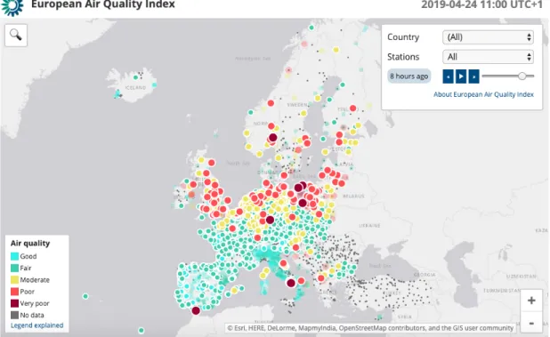
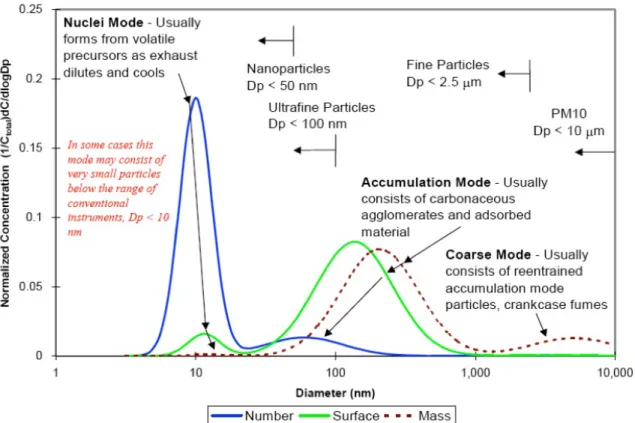
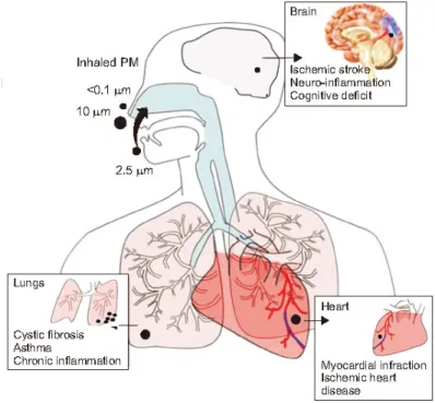
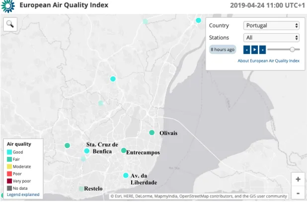
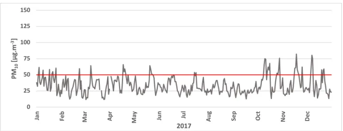
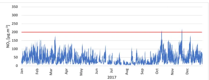
Figure 1.1: Schematic representation of the structure of the thesis. ... 26 Figure 2.1: Diagram representation of air pollutants path in atmosphere, from their emission to their impacts on people and environment (https://www.eea.europa.eu/publications/explaining-road-transport-emissions). ... 27 Figure 2.2: Health effects of air pollution regarding the seriousness of the effects and the number of people affected (adapted from EEA, 2014). ... 28 Figure 2.3: EU urban population exposed to air pollutant concentrations above air quality standards of the EU Air Quality Directive (top) and WHO air quality guidelines (bottom). (Adapted from EEA, 2018a). ... 38 Figure 2.4: Daily PM10 concentrations in Europe, in 2016. The map shows the 90.4 percentile of the PM10 daily mean concentrations, representing the 36th highest value in a complete series. It is related to the PM10 daily limit value, allowing 35 exceedances of the 50 µg.m-3 threshold over 1 year. Red and purple dots indicate stations where concentrations were higher than the daily limit value (50 µg.m-3). (EEA, 2018a). ... 39 Figure 2.5: Annual PM10 concentrations in Europe, in 2016. Red and purple dots indicate stations where concentrations were higher than the daily limit value (40 µg.m-3). Green dots indicate stations reporting values below the WHO AQG for PM10 (20 µg.m-3). Only stations with more than 75 % of valid data have been included in the map (EEA, 2018a). ... 40 Figure 2.6: Annual PM2.5 concentrations in Europe, in 2016. Red and purple dots indicate stations where concentrations were higher than the daily limit value (25 µg.m-3). Green dots indicate stations reporting values below the WHO AQG for PM2.5 (10 µg.m-3). Only stations with more than 75 % of valid data have been included in the map (EEA, 2018a). ... 40 Figure 2.7: European AQMN showing air quality index in Europe on the 24th April 2019 at 11:00 UTC (http://airindex.eea.europa.eu/). ... 41 Figure 2.8: Classification of particulate matter (PM10, PM2.5 and PM0.1 or UFP) and its common sources (Mühlfeld et al., 2008). ... 43 Figure 2.9: Schematic representation of PM according to its size (https://www.epa.gov/pm-pollution/particulate-matter-pm-basics). ... 44 Figure 2.10: Typical engine exhaust size distribution in mass, surface and number weightings (adapted from Kittelson, 1998). ... 45 Figure 2.11: Total concentrations of trace elements and metals bounded to PM0.25 found in two different locations of Los Angeles. Error bars represent standard deviation (from Shirmohammadi et al., 2018). .... 48 Figure 2.12: Diagrammatic representation of inhaled particulate matter of variable sizes and PM-linked respiratory, cardiovascular, and neurological diseases (adapted from Zaheer et al., 2018) ... 49 Figure 3.1: PM10 (top) and NO2 (bottom) relative emissions, in Lisbon, 2014, by source (FCT-NOVA, 2017). ... 55 Figure 3.2: AQMN in Lisbon and respective air quality index on the 24th April 2019 at 11:00 UTC (http://airindex.eea.europa.eu/). ... 56 Figure 3.3: Annual average concentrations of PM10 and NO2 in Av. da Liberdade (AL) and Entrecampos (EC) AQMS and limit value established in EU (2008). ... 57 Figure 3.4: Annual average concentrations of PM2.5 in Olivais (OLI) and Entrecampos (EC) AQMS and limit value established in EU (2008). ... 58 Figure 3.5: Daily average concentrations of PM10 in Av. da Liberdade, in 2017. The red line represents the LV (EU, 2008). ... 59 Figure 3.6: Daily average concentrations of PM10 in Entrecampos, in 2016. The red line represents the LV (EU, 2008). ... 59 Figure 3.7: Hourly average concentrations of NO2 in Av. da Liberdade, in 2017. The red line represents the LV (EU, 2008). ... 59
Figure 3.8: Hourly average concentrations of NO2 in Entrecampos, in 2017. The red line represents the LV (EU, 2008). ... 60 Figure 3.9: Number of exceedances of daily PM10 and annual NO2 limit values in Av. da Liberdade and Entrecampos between 2010 and 2017. The red line represents the annual number of exceedances allowed for each one of the pollutants (35 and 18 days for PM10 and NO2, respectively) (EU, 2008). ... 60 Figure 3.10: LEZ geographical extent and location (adapted from Ferreira et al., 2015). ... 61 Figure 3.11: Distribution of vehicles by type and zone in 2015 (adapted from Henriques, 2015). ... 62 Figure 3.12: Relative distribution of Euro Standard by type of vehicle and zone in 2015 (adapted from Henriques, 2015). ... 63 Figure 3.13: Distribution of NOx and PM emission by type of vehicle in Av. da Liberdade in 2015 (adapted from Henriques, 2015). ... 64 Figure 3.14: Distribution of light passenger and light duty vehicles by engine capacity (adapted from Henriques, 2015). ... 64 Figure 3.15: Representation of Lisbon Airport (dashed contour) on map (Maps source: https://www.google.pt/maps). ... 65 Figure 3.16: Map of the network of ferry stations connecting the northern and southern shores of Tagus River (Maps source: https://www.google.pt/maps, last accessed on December 2018). ... 66 Figure 3.17: Power, in kW, by type of ferry of the fleet operating in Tagus River, in LMA. ... 67 Figure 3.18: Hourly number of ferries cruising in Tagus, LMA, by week-day, Saturday and Sunday/Holiday. ... 67 Figure 3.19: Annual average trips in 2018 associated with the different connections. ... 67 Figure 3.20: Particle number counter device, P-Trak®. ... 68 Figure 3.21: LEZ geographical extent and location of the three analysed sites (black dots) (adapted from Ferreira et al., 2015). ... 69 Figure 3.22: Representation of sampling sites. The star indicates the AQMS and sampling sites (a) Avenida da Liberdade, site 1; (b) Entrecampos, site 2 and (c) 2nd Circular, site 3, where dots indicate the two different locations (Torres de Lisboa and Escola Alemã, sites 3.1 and 3.2, respectively). (Maps source: https://www.viamichelin.pt/web/Mapas-plantas). ... 71 Figure 3.23: Representation of LA and sampling sites. The thin arrow indicates the main runway and direction of landings and take-offs, the dashed line shows the landing and take-off route, and the thick arrow, on top left, indicates the predominant wind direction. (Maps source: https://www.google.pt/maps). ... 74 Figure 3.24: Location of the ferry-related sampling sites (dots). Arrows indicate the downwind directions to cruising paths; Shadow triangles indicate the manoeuvring area; continuous lines indicate the ferry path. Top left – Cacilhas; top right – Barreiro; bottom left – Montijo and bottom right – Seixal. (Maps source: https://www.viamichelin.pt/web/Mapas-plantas#, last accessed on December 2018). ... 77 Figure 4.1: Boxplot of 1-minute PNC mean distribution by traffic site. (1st quartile, average (x), median (-), 3rd quartile and outliers (dots)). ... 82 Figure 4.2: Traffic characterization by type of vehicle in Av. da Liberdade over two periods during sampling. (PC – passenger cars; LD – light-duty vehicles; T – taxis; B – buses; HD – heavy-duty vehicles; G – gasoline; D – diesel; HE – hybrid or electric). ... 83 Figure 4.3: Traffic characterization by Euro Standard and type of vehicle . (PC – passenger cars; LD – light-duty vehicles; T – taxis; B – buses; HD – heavy-duty vehicles; G – gasoline; D – diesel; HE – hybrid or electric) in Av. da Liberdade. ... 84 Figure 4.4: Association between 1-minute PNC peaks and specific observed vehicles in Av. da Liberdade. The black arrow denotes a period where measurements were discarded due to another source of contamination. ... 85 Figure 4.5: 1-hour means of PNC vs. buses and light-duty vehicles, in Av. da Liberdade ... 86 Figure 4.6: Statistical outputs for regression analysis with 95% confidence level between PNC 1-hour averages and the number of vehicles, in Entrecampos. ... 86
Figure 4.7: Association between 1-minute means of PNC peaks and specific observed vehicles in
Entrecampos. ... 87
Figure 4.8: Statistical outputs for regression analysis with 95% confidence level between PNC 15-minutes averages and air pollutants (NO, NO2, NOx and PM10) monitored in AQMS of Av. da Liberdade. Regression for nitrogen oxides was done with PNC 15-minutes averages and with 1-hour averages for PM10. ... 88
Figure 4.9: Statistical outputs for regression analysis with 95% confidence level between PNC 1-hour averages and PM10 monitored in AQMS of Entrecampos. ... 89
Figure 4.10: Statistical outputs for regression analysis with 95% confidence level between PNC 1-hour averages and wind speed, in Av. da Liberdade. ... 90
Figure 4.11: As in Figure 4.10 but respecting to Entrecampos. ... 90
Figure 4.12: 10-minute PNC averages obtained under impact wind direction (blue) and non-impact wind direction (grey). Sites are ordered by distance to runway and type of location. ... 94
Figure 4.13: Overall statistical outputs for regression analysis with 95% confidence level between PNC 10-minutes averages and the number of landings. ... 96
Figure 4.14: As in Figure 4.13 but respecting to the number of take-offs. ... 97
Figure 4.15: As in Figure 4.13 but respecting to the number of flights (landings and take-offs). ... 97
Figure 4.16: As in Figure 4.13 but respecting to wind intensity. ... 97
Figure 4.17: Boxplot of 10-minutes PNC mean distribution by site ordered by location and increase distance to LA (please see sites spatial distribution in Figure 3.23b). (1st quartile, average (x), median (-), 3rd quartile and outliers (dots)). ... 98
Figure 4.18: LA-related PNC geographical distribution: minimum, average and maximum (PNC expressed in pt.cm-3). ... 99
Figure 4.19: PNC concentrations at five sites located in LA landing route vicinity, ordered by increasing distance to the runway (a), and corresponding wind speed and ML height (b). ... 100
Figure 4.20: UFP concentration at sampling site 5 (LA vicinity) and LTO cycles differentiated by long-haul flights and low/medium-long-haul flights. ... 101
Figure 4.21: (a) 10-minutes UFP average concentration, number of flights and wind direction, in LA vicinity (site 5) (b) Geographical detail of sampling site: relative position to the beginning of the runway (small dashed red arrow) and to aircrafts idling to take-off (pointed orange arrow). The runway is represented by the black arrow and idling path by the large dashed blue line. ... 102
Figure 4.22: UFP concentration at sampling site 13 (landing path, far from LA), wind direction and number of landings during a 10-minutes period. ... 103
Figure 4.23: Boxplot of 1-minute PNC mean distribution by ferry-related site, under downwind conditions. (1st quartile, average (x), median (-), 3rd quartile and outliers (dots)). ... 105
Figure 4.24: Site by site PNC during the immediate eight minutes before/after ferry operations (blue), eight minutes before departures (grey), eight minutes after arrivals (yellow). ... 106
Figure 4.25: Average PNC of ferries from/to Barreiro measured in Seixal as function of wind speed and under wind direction range from N to NE. ... 107
Figure 4.26: Detail of Barreiro and Seixal geographical location. Plumes emitted by Barreiro’s ferries affect PNC on Seixal when wind direction range from NE to NW. Shadowed triangle shows the wind direction range in which only plumes emitted by Barreiro’s ferries are measurable in Seixal; the continuous and dashed lines show the ferries paths from Barreiro and Seixal, respectively. ... 108
Figure 4.27: PNC rose pollution in each ferry station (pt.cm-3 x 10³). ... 109
Figure 4.28: Obtained PNC average for different class of ferry operating among the four stations studied, downwind. ... 109
LIST OF TABLES
Table 2.1: Implementation of Euro Standards by vehicle’s category. ... 31
Table 2.2: Average dimension (nm) and concentration (pt.cm-3) of atmospheric particles in European cities (adapted from Hofman et al. (2016) and Kumar et al.). ... 32
Table 2.3: LTO cycle phases defined by ICAO (ICAO, 2011). ... 33
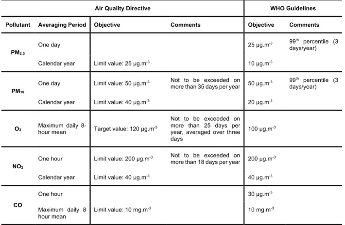
Table 2.4: Air quality standards under the EU Air Quality Directive and WHO air quality guidelines (adapted from EEA, 2018b). ... 36
Table 2.5: National ambient air quality standards established by USEPA (adapted from https://www.epa.gov/criteria-air-pollutants/naaqs-table). ... 37
Table 2.6: Premature deaths and years of life lost (YLL) attributable to PM2.5 and NO2 exposure in EU-28 and in 41 European countries, in 2015 (adapted from EEA, 2018a). ... 52
Table 3.1: Technical characteristics of Lisbon urban AQMS (http://www.ccdr-lvt.pt/pt/avaliacao-da-qualidade-do-ar-na-rlvt/8085.htm#D1). ... 57
Table 3.2: Emissions of PM10 and PM2.5 in 2014 regarding the four main ferry connections between Lisbon and South Tagus shore. ... 66
Table 3.3: P-Trak® technical characteristics (adapted from P Trak®, 2013). ... 69
Table 3.4: Geographic coordinates of traffic-related sites. ... 70
Table 3.5: Geographic coordinates of each LA-related site. ... 74
Table 3.6: Geographic coordinates of each ferry-related site. ... 77
Table 3.7: Technical characteristics of the portable meteorological station WatchDog 2700. ... 78
Table 3.5: Technical data of the ships identified during sampling periods (https://ttsl.pt/terminais-e-frota/frota/) ... 79
Table 4.1: Sampling dates and periods for each road traffic-related site and the corresponding height of the mixing layer (ML), wind speed (v) and direction, temperature (T), relative humidity (RH) and measured minimum (Min), mean, mode, and maximum (Max) PNC values. ... 81
Table 4.2: Obtained average, mode and standard deviation (SD) of PNC on traffic-related sites, in pt.cm-3 x 10³. ... 82
Table 4.3: Single factor ANOVA for PNC sampled values among the four traffic sites ... 83
Table 4.4: Summary of statistical outputs for regression analysis with 95% confidence level between PNC and other pollutants and meteorological parameters, in Av. da Liberdade and Entrecampos. ... 91
Table 4.5: Sampling date and period for each airport-related site and the corresponding height of the Mixing Layer (ML), wind speed (v) and direction, temperature (T), relative humidity (RH) and measured minimum (Min), mean, mode, and maximum (Max) PNC values. ... 92
Table 4.6: Average, mode and standard deviation (SD) of PNC on airport-related sites, in pt.cm-3 x 10³. Sites are arranged by location and distance to the airport. ... 93
Table 4.7: Impact wind directions (IWD, in º) by site. ... 94
Table 4.8: Single factor ANOVA among all sites. ... 95
Table 4.9: Single factor ANOVA among sites with similar characteristics. ... 96
Table 4.10: Sampling date and period for each ferry-related site and the corresponding height of the Mixing Layer (ML), wind speed (v) and direction, temperature (T), relative humidity (RH) and measured minimum (Min), mean, mode, and maximum (Max) PNC values. ... 104
Table 4.11: Obtained average, mode and standard deviation (SD) of PNC on ferry-related sites, in pt.cm-3 x 10³. ... 104 Table 4.12: Obtained results of PNC increase with ferry operations, regression analysis between PNC averages and ferry occurrences and wind speed and ANOVA analysis between periods with and without ferry operations. ... 107
1 INTRODUCTION
1.1 B
ACKGROUNDAir pollution, mainly in great urban areas, had become a major problem over the past years. Urban air pollution is mostly associated with the transport sector. The main primary pollutants are airborne particulate matter (PM), nitrogen oxides (NOx, mostly nitrogen monoxide, NO, and nitrogen dioxide, NO2, often expressed as NO2), uncombusted hydrocarbons (HC) and carbon monoxide (CO) (Kousoulidou et al., 2008). Many studies identify road traffic related emissions as the main responsible for air quality degradation in urban areas (e.g. Anenberg et al., 2017). Even with improved exhausting systems, due to higher traffic levels, air pollution should keep an increasing tendency in certain regions of the world (WHO, 2005). Also, some authors have been studied other contributions, such as tire-road interference in ultrafine particulate emissions. Ultrafine particles are generated under extreme driving conditions, i.e., full stop braking, at the tire road interface (Mathissen et al., 2011). Considering other transport modes, such as airports, maritime traffic and in-land passenger ferries currently using combustion engines are also responsible for emissions of particulate matter, nitrogen oxides, carbon monoxide and volatile organic compounds (VOC) which contribute for a deterioration of air quality (Anenberg et al., 2017; Hagler et al., 2010; Kousoulidou et al., 2008; López-Aparicio et al., 2017; Sardar et al. 2005; Stafoggia et al., 2016; Zhu et al., 2002a,b).
According to the World Health Organization (WHO) particulate matter database, more than 80% of people living in urban areas where air pollution is monitored are exposed to air pollution that exceed WHO’s air quality limits (WHO, 2018). The database, which currently covers 4300 cities in 108 countries, points that 97% of cities in low and middle-income countries with more than 100 000 inhabitants do not meet WHO air quality guidelines, whereas in in high-income countries the percentage decreases to 49%. The increase in air pollution levels monitoring recognizes their association with health impacts: as urban air quality declines, the risk of stroke, heart disease, lung cancer, and chronic and acute respiratory diseases, including asthma, increases for the people who live there. Moreover, WHO estimates a worldwide 4.2 million deaths every year as a result of exposure to ambient air pollution and that 91% of the world’s population lives in areas where air quality exceeds the global defined guidelines limits for PM10 and PM2.5 (particulate matter with aerodynamic diameter less than 10 µm and 2.5 µm, respectively) annual means: 20 µg.m-3 for PM10 and 10 µg.m-3 for PM2.5. (WHO, 2006). Course particles (PM10) are inhalable, and they can easily reach people’s lungs and fine particles (PM2.5) may even entering the bloodstream.
Over the past years, specific components of PM came into focus: ultrafine particulate matter (UFP), which consists in particles with aerodynamic diameter less than 0.1 µm (100 nm).The urban main source of UFP is also combustion engines and they are able to reach cellular level and cause intracellular damages (Carosino et al., 2015). However, the impact of UFP on human health is still under studying and the results
are inconclusive, despite the possibility of being even more harmful than fine particles (PM2.5) (Lanzinger et al., 2016).
Behind particulate matter, nitrogen oxides, carbon monoxide, volatile organic compounds and tropospheric ozone (O3) must also be taken in consideration due to their negative and sometimes synergetic impacts on air quality (AQ). Nitrogen oxides are linked to respiratory problems, mucous tissues irritation and central nervous system damages. In particular, nitrogen oxide, has been linked to premature mortality and morbidity in result of cardiovascular and pulmonary diseases. Carbon monoxide is considered toxic once it may connect to haemoglobin and disable its ability to bloodstream transport oxygen from lungs to cells. Depending on their chemical nature, VOCs effects on human health may vary from simple olfactive discomfort to breathing problems and even carcinogenic effects. Ozone is a secondary pollutant and therefore in urban areas, is mainly produced in the presence of sunlight (wavelength less than 400 nm) by photochemical reactions where volatile organic compounds are oxidized by nitrogen oxides, both emitted by combustion engines. Moreover, ozone is the major component of photochemical smog and it is related to respiratory diseases such breathing problems, asthma and reduced lung function. Aside these health issues, tropospheric ozone is a short-lived greenhouse gas. Additionally to their role as ozone precursors, VOC and NOx are dangerous air pollutants themselves (
http://www.ccdr-lvt.pt/pt/o-ar-e-os-poluentes-atmosfericos/8082.htm). Furthermore, particulate matter interferes with the radiative budget and albedo and therefore has impact on climate; nitrogen oxides are responsible for acidification and both ozone and volatile organic compounds are harmful to vegetation.
When speaking about air quality is not controlled exclusively by the amount of pollutants emitted. Meteorological conditions play also a crucial role in transport, transformation and dispersion processes of atmospheric pollutants. Additionally, these processes are affected by local topography and meteorological factors such as wind intensity and direction, atmospheric pressure, temperature, precipitation and solar radiation (Mu et al., 2011; Pateraki et al., 2012; Shen et al., 2009; Tai et al., 2010; Wang et al, 2018),
Pollutants dispersion in the atmosphere are mainly driven by wind speed and direction. On one hand, wind speed generates mechanical turbulence, which is responsible for local dispersion. Therefore, low wind speeds lead to high pollutants concentration and moderate wind speeds promote their dispersion, lessening their ambient concentrations. On the other hand, strong wind may induce vortices’ effects which might lead to high pollutants concentration in the predominant wind direction, downwind to the source(s) (Grundström, 2015; Guldmann, 2011; Hudda et al., 2018; Kim and Guldmann, 2011; Russo et al., 2014a). Regarding atmospheric pressure, low pressure systems (cyclones) are generally associated to atmospheric high turbulence, enhancing pollutants dispersion and lessening ground level pollutants concentration. On the contrary, high pressure systems (anticyclones), characterized by week winds and atmospheric stability, inhibit the pollutants dispersion, increasing their ground level concentrations (Lin et al., 2009). Moreover, temperature plays an important role in their vertical atmospheric dispersion by inducing ascendant convection (lessen ground level concentrations). As an example, in Summer, the high temperatures promote the
tropospheric ozone production. On the other hand, in Winter, the occurrence of thermal inversions may lead to ground-level high pollutants concentrations. The role of precipitation on pollutants dispersion is also noticeable, as precipitation is usually associated to an instable atmosphere, promoting air pollutants dispersion. Rain droplets solubilize gaseous pollutants and particulate matter, accelerating their deposition on surface (wet deposition), decreasing their atmospheric concentrations (Shen et al., 2009). Finally, strong solar radiation, associated with high temperatures, promotes photochemical reactions and enhances secondary pollutants production, such as ozone.
As pointed out before, road traffic is one of the main contributors to air pollution in urban areas (Anenberg et al., 2017; Lee et al., 2017; Keuken et al., 2016). The exhaust gases emitted close to the surface often lead to air quality degradation, once road traffic is characterized by the emission of toxic particles and gases (Russo and Soares, 2013). Despite all the efforts that have been made, Lisbon still has an intense road traffic and some areas often exceed the legal standards, mainly regarding particulate matter and nitrogen dioxide (Ferreira et al, 2015). Other emission source, less addressed in previous studies, is the activity of the aviation industry where there are no detailed studies of the impact of Lisbon Airport Humberto Delgado (LA) on its surroundings regarding particulate matter concentration, namely UFP, and other atmospheric pollutants. Another transport related sector with no air quality impact information due to the lack of previous studies is in-land passenger ferries. Transport sector is also expected to be responsible for the emission of air pollutants with significant impact on air quality, namely UFP.
This thesis is focused on UFP concentration over the urban region of Lisbon and its relationship with transport-services. In the last decade, several studies have been carried out in order to characterize air quality in different European cities, namely trying to distinguish the range of average UFP concentrations in those European cities (Hofman et al., 2016; Kumar et al., 2014). Lisbon is a city with 547 733 inhabitants, according to the last cense (INE, 2011).
The appellative climate (temperature warm), together with its location, close to one of the major estuaries in Europe and to Atlantic Ocean, rich historical monuments and gastronomy, makes Lisbon one of the most attractive European cities. Therefore, the tourist sector is one of its main economic activity. Besides, many people travel daily to Lisbon, mostly for working and school/university formation. These conjugated factors contribute to an increase in the different transport modes, making transports (road-traffic, aircrafts and in-land passenger ferries) the main air pollution source in the city, like in many other cities, as previously pointed out by several studies (e.g. Lee et al., 2017; López-Aparicio et al., 2017; Stafoggia et al., 2016). Furthermore, the Lisbon Airport is located within the city and there is a considerable number of passenger river transports to and from Lisbon, particularly during weekdays.
During recent years, several studies have been carried out in order to evaluate air quality in Lisbon (e.g. FCT-NOVA, 2017; Monjardino et al., 2018; Lopes et al., 2019a,b; Russo et al., 2014a,b). Also, several measures have been implemented in areas considered critical (downtown) in order to contribute to air quality improvement (Ferreira et al., 2015; Monteiro et al., 2015). However, there is a lack of studies to assess UFP
levels, which are mainly emitted by combustion engines. This work intends to fill this gap and is the first work on characterization of UFP concentration in Lisbon. It will allow to evaluate not only the UFP concentrations but also to estimate the potential level of exposure of the affected population. One of the main contributors to air pollution in Lisbon is road traffic (Russo and Soares, 2013), which is characterized by the emission of toxic particles and gases. However, considering the location of Lisbon Airport and the amount of ferries crossing Tagus River, aircrafts and in-land passenger ferries are also a pertinent emission source, far less addressed in those studies.
Therefore, this study intends to fill the above-mentioned information gaps, assessing the effect on UFP concentrations of road, air and river traffic modes in Lisbon. These three sources assume special relevance due to their locations (within or close to the city centre, proximity to residential, business, services and recreational areas, schools, sport complexes, hospitals and companies, among others) and, therefore, the number of people potentially affected, particularly by peak concentrations. Furthermore, given the lack of studies in airport-related UFP concentrations in the immediate airport’s vicinity, it also aims to assess the airport-related UFP concentrations in the immediate LA vicinity. This study also proposes to assess when and how much air traffic in LA affects UFP concentrations taking into consideration the aircraft types (short/medium or long-haul) and the associated movement (landing or take-off). A thorough analysis on UFP emissions on the vicinity of the LA will improve the ability and capability of alert system for air quality in Lisbon. In the case of in-land ferries, according to the literature review, there is an almost total lack of studies characterizing UFP concentrations in ferries stations and across ferries path. In Lisbon, there are no previous studies on this subject which assumes special relevance, once it is a significant transport mode used to connect Tagus shores.
Finally, the thesis will use the collection of data to provide further relevant insights on monitoring strategies of UFP and a better understanding of the relationships between UFP and other pollutants, including the decisive role of meteorological parameters during data collection and further interpretation.
1.2 R
ESEARCHQ
UESTIONS ANDO
BJECTIVESThe main objective of this thesis is to set up a monitoring scheme and evaluate different modes of traffic related UFP concentrations in Lisbon. For that purpose, the present work aims to access the contribution of UFP emissions of three main sources (road-traffic, aircrafts and in-land passenger ferries) to their atmospheric concentration. In this context, the research questions are:
RQ1. Regarding vehicles, aircrafts and ferries traffic, what are the UFP levels in Lisbon in the proximity of these sources?
RQ2. How can we design appropriate monitoring techniques to evaluate UFP levels at roadside, airport landing and take-off pathways, and close to ferries stations?
RQ4. Is it possible to establish and quantify relationships between UFP levels and traffic intensity (vehicles, aircrafts and ferries)?
RQ5. Regarding road traffic, are there any correlations between UFP concentrations and other pollutants monitored by air quality monitoring stations in the vicinity?
To achieve the thesis objectives and answer these research questions, the following particular tasks have been accomplished:
- Collecting UFP concentrations in order to cover the different traffic sources considered and their influence;
- Compiling information on the traffic intensity associated with the different sources under research such as the number and type of vehicles, number of flights and aircraft type and movements, and number of in-land passenger ferries during sampling periods;
- Monitoring/Recording meteorological conditions during sampling periods.
1.3 S
TRUCTURE OF THET
HESISThis thesis is divided in five chapters as following:
• Chapter 1 – Introduction, where the aim and contextualization of the present work is defined as well as the research questions.
• Chapter 2 – Literature Review, is divided into sub-chapters according to the different contexts: air pollution in urban areas, the main air pollution sources in urban areas, guidelines and monitoring of air quality focused on particulate matter, UFP impacts on health and climate and influence of meteorology on air quality.
• Chapter 3 – Background and Methodology, begins by contextualization of our case study, Lisbon and describes the methodology applied on sampling and data analysis for each one of the three sources considered.
• Chapter 4 – Results and Discussion, as its title suggests, presents the obtained results and their discussion, also by source.
• Finally, Chapter 5 – Conclusions, presents the main achieved conclusions, both by source and global. The main limitations and suggestions for future works are also indicated.
Figure 1.1 presents the schematic structure of this document. The work developed in this dissertation resulted in one conference paper and presentation and two peer reviewed publications:
Figure 1.1: Schematic representation of the structure of the thesis.
Publications:
Lopes, M., Russo, A., Monjardino, J., Gouveia, C., Ferreira, F. (2019). Monitoring of ultrafine particles in the surrounding urban area of a civilian airport. Atmospheric Pollution Research. ISSN 1309-1042.
https://doi.org/10.1016/j.apr.2019.04.002.
Lopes, M., Russo, A., Gouveia, C., Ferreira, F. (2019). Monitoring of ultrafine particles in the surrounding urban area of ferries terminals. Journal of Environmental Protection. Vol. 10, 838-860
https://doi.org/10.4236/jep.2019.106050. Conference:
Lopes, M., Corrêa, M., Ferreira, F., “Avaliação do Impacte do Aeroporto de Lisboa na Concentração de Partículas Ultrafinas na Zona Urbana Circundante”, Livro de Atas da Conferência Internacional de Ambiente em Língua Portuguesa (CIALP), do XX Encontro da Rede de Estudos Ambientais de Países de Língua Portuguesa (REALP) e da XI Conferência Nacional do Ambiente, Aveiro, 8-10 de maio de 2018, ISBN: 978-972-789-540-3, Vol-III, pp. 235-244.
1. Introduction
Background and Context Research Questions and Objective
Structure of the Thesis
2. Literature Review
Air Quality in Urban Areas (Road-Traffic, Aircrafts, Ships) Guidelines and Monitoring of PM
Particulate Matter (Formation, Composition, Main Sources, Classification...)
Impacts of PM on Human Health and Climate Influence of Meteorology on Air Quality
3. Background and Methodology
Charaterization of our cae study: Lisbon Sampling Equipment Monitoring Campaigns Meteorological Data Data Analysis 4. Results and Discussion
Statistical Analysis (e.g. traffic frequency vs. UFP levels) Analysis of Meteorological Paremeters Influence on UFP levels
5. Conclusions
By source conclusions Answer to Research Questions
Main constrainments Suggestions for future works
2 LITERATURE
REVIEW
2.1 A
IRQ
UALITY INU
RBANA
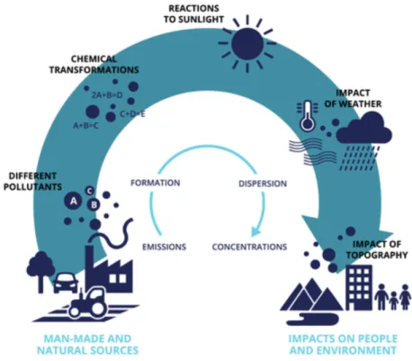
REASAir quality is usually used to express the degree of pollution of the air we breathe. This pollution is caused by a mixture of chemical substances emitted in ambient air or as a result of chemical reactions among them or with ambient air constituents (Brimblecombe, 1999) as exemplified in Figure 2.1. Air pollution, mainly in great urban areas, had become a major problem over the past decades. Atmospheric pollution is mostly associated with traffic and its main primary pollutants: particulate matter, nitrogen oxides, uncombusted hydrocarbons and carbon monoxide (Kousoulidou et al., 2008). Many studies identify road traffic related emissions as the main contributor to poor air quality in urban areas (Anenberg et al., 2017; Kumar et al., 2014; Pant and Harrison, 2013; Querol et al., 2008; Stanier et al., 2004a).
Figure 2.1: Diagram representation of air pollutants path in atmosphere, from their emission to their impacts on people
and environment (https://www.eea.europa.eu/publications/explaining-road-transport-emissions).
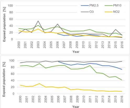
Regarding Europe, the last report of European Environmental Agency (EEA) on Air Quality in Europe highlights that, in 2016, traffic-related pollutants (PM10, PM2.5, O3, and NO2) exceeded both the EU limit values and the World Health Organization (WHO) guidelines (EEA, 2018a). In 2016, 13 % of EU-28 urban population resided in areas where the European Union (EU) daily limit value of PM10 was exceeded, 6 % of the EU-28 urban population was exposed to PM2.5 levels above the EU limit, 12 % of the urban population was exposed
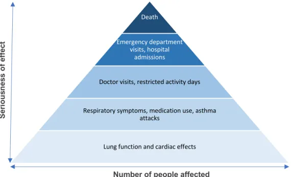
to O3 concentrations above the EU target value threshold, and 7 % of urban population resided in areas where the annual EU limit value of NO2 was exceeded (EEA, 2018a). According to this report, in 2015, approximately 422 000 deaths in Europe were related to PM2.5 (originating from long-term exposure), 391 000 of which were in the EU-28. The same report points out that, in 2016, 42 % of UE-28 urban population was exposed to PM10 levels exceeding the stricter World Health Organization (WHO) air quality guidelines (AQG), 74 % of UE-28 urban population was exposed to PM2.5 concentrations exceeding the WHO AQG, 98 % of UE-28 urban population was exposed to O3 levels above the WHO AQG, and 7 % of the UE-28 urban population lived in areas where the NO2 WHO AQG was exceeded (EEA, 2018a). The health effect pyramid of air pollution is outlined in Figure 2.2.
Figure 2.2: Health effects of air pollution regarding the seriousness of the effects and the number of people affected
(adapted from EEA, 2014).
The WHO had recently estimated around 4.2 million deaths worldwide due to air pollution exposure (WHO, 2018). The same source points out that in 2016, 91 % of world population was living in areas where WHO air guideline levels were not met. Particulate matter (PM) is one of the major causes of premature deaths (Gakidou et al., 2017). According to this study, PM is the sixth cause of death, in a list of 84 risk factors, and is pointed as the cause of 4 million deaths in 2016.
Different emission sources have different contributions on ambient air pollutants concentrations. Concentrations not only depend on the amount of pollutant emitted, but also on proximity to source, emission conditions (e.g. height and temperature) and other factors (e.g. dispersion conditions and topography). Low emission heights, such traffic, are generally associated to higher significant impact on ground concentrations than emissions from high stacks (EEA, 2018b).
Death
Emergency department visits, hospital
admissions
Doctor visits, restricted activity days
Respiratory symptoms, medication use, asthma attacks
Lung function and cardiac effects
Se ri o u sn es s o f ef fe ct
Besides road traffic, other air pollution sources pointed by several authors are air traffic (e.g. Stafoggia et al., 2016) and maritime transport (e.g. Westerlund et al, 2015). In this last source, López-Aparicio et al. (2017) find domestic ferries as the main contributors to emissions among harbour ships.
2.1.1 Road Traffic
Road traffic is the most important contributor to air pollution in urban areas (Anenberg et al., 2017; Keuken et al., 2016; Kumar et al., 2014; Lee et al., 2017; Morawska et al., 2008; Rönkkö et al., 2017). Therefore, as referred by Joerger and Pryor (2018), people living, working or spending much time next to intense traffic roads are exposed to high traffic-related emissions and have higher risk to respiratory and cardiovascular health problems or even premature mortality (Chen et al., 2008; Chen et al., 2017; HEI, 2013; Hystad et al., 2015; Lelieveld et al., 2015). Combustion generated particles (from vehicle emissions) range from 30 nm to 500 nm (Vu et al. 2015). Several studies have concluded that the elevated particle number concentrations decay exponentially with increasing distances from the roadway (e.g. Zhu et al., 2009). Nucleation (atmospheric formation of new particles) (Kulmala et al., 2014) also plays an important rule to UFP concentrations in urban areas (Brines et al., 2015; Kulmala et al., 2017; Stanier et al., 2004b; Watson et al., 2006).
Particulate matter emitted from gasoline and diesel engines consist mainly on ultrafine particles with size ranges of 20 to 60 nm and 20 to 130 nm, respectively (Karjalainen et al., 2014; Morawska et al., 2008;). UFP represent only 0.1 to 10% of the total particulate mass, despite might represent more than 90% of the total particle number (Giechaskiel et al., 2010). Particle emission depends on the fuel, engine technology and aftertreatment devices. Compared to the standard gasoline passenger cars, gasoline direct injection technology induces an increase of UFP concentration (Köhler et al., 2013; Liang et al., 2013).
Research suggests that a significant fraction of a person's total daily exposure to fine and ultrafine particles occurs during commuting periods (Ham et al., 2017). Transport microenvironments (MT), close to traffic emissions sources, exhibit higher traffic related pollutants concentrations (Goel and Kumar, 2014; Patton et al., 2016). In their commuting to work, school and shopping, among other activities, people spend a variable, but considerable, amount of time in vehicles (cars, public transportation, motorcycles or bicycles) or close to them. Due to recurrent acceleration and deceleration of vehicles, intense-traffic areas are susceptible to have higher emissions (Goel and Kumar, 2015). A study carried out by De Nazelle et al. (2012) concluded that UFP concentrations in cars are 2-3 times higher than in walk or bike modes, close to roadways. Still, considering inhalation, pedestrians and cyclists’ doses are comparable to car drivers. In Europe, results show that car riders are exposed to the highest levels of UFP; on the contrary, pedestrians are exposed to the lowest levels (De Nazelle et al., 2017). However, in modern cars, equipped with high-efficiency filters and air recirculation, the UFP exposure levels inside vehicles are significantly lower (Spinazzè et al., 2014). Still according to this study, the highest exposures were observed for walking or biking along high-trafficked routes and while using public buses.
Many air monitoring studies (Hagler et al., 2010; Sardar et al., 2005; Zhu et al., 2002a,b) conducted near traffic roads or on-roadways has focused not only on the UFP measurements, but particularly on emissions of more conventional and well-studied pollutants such as:
• Carbon monoxide (CO): the adoption of emission control technologies and regulations allowed ambient concentrations of this pollutant to decline over the past years. However, mostly light-duty and gasoline vehicles remain as the primary source of CO at most locations.
• Nitrogen oxides (NOx): diesel vehicles are responsible for the majority of NOx emissions. The majority of NOx exhaust occurs as NO (primary emissions). Once in atmosphere, NO is rapidly oxidized to NO2 (a secondary pollutant), which is the focus of concern in terms of health effects. Heavy-duty diesel engines with after-treatment equipment may contain a greater ratio of NO2/NO.
• Particulate matter (PM10, PM2.5): significant near-roadway sources of PM mass include direct emissions from vehicle combustion engines (predominantly PM2.5), brake and tyre wear, and resuspension of dust from the road surface (mostly PM10 and larger). PM2.5 atmospheric concentration is mostly affected by contributions from regional sources. Therefore, the impact of direct emissions from motor vehicles is generally small in near-roadway environments.
• Volatile organic compounds (VOC) and carbonyls: these compounds are emitted from both natural and anthropogenic sources, including vehicles engines. They are involved in the photochemical formation of tropospheric O3. Moreover, some of them have been associated with toxic health effects. VOC of concern for near-road monitoring include benzene, toluene, ethylbenzene, xylenes, styrene, formaldehyde, acetaldehyde, and acrolein.
• Black or elemental, carbon (BC or EC): often referred to as “soot,” is a common constituent emitted by vehicles engines. BC represent the black (graphitic) portion of PM. Though heavy-duty diesel engines are often pointed as the main sources of BC, all combustion engines emit BC. A study conducted by Liggio et al. (2012) has shown that BC emissions from light-duty gasoline vehicles are expected to be at least a factor of 2 to 9 times higher than formerly supposed. In urban areas, the main source of BC is diesel trucks engine which rules near-roadway environments.
Aiming to minimize traffic-related air pollution in urban areas, some plans and/or particular measures have been taken to reduce air pollutant concentrations to acceptable levels, meeting the EU limit values and WHO guidelines. The implementation of Low Emission Zones (LEZ), areas where the circulation of most polluting vehicles is restricted or penalized on the basis of European class emission standards, are often used as the major component of emission control strategies. London, UK, introduced the world's largest citywide LEZ in 2008 (Mudway et al., 2019). Currently, there are about 264 LEZ across Europe (Santos et al., 2019). Also, in Asia, including Singapore and Tokyo, LEZ are being implemented (Mudway et al., 2019). Restrictions in vehicles circulation range from only heavy duty to all type of vehicles according to their Euro Standard (Table 2.1).
Table 2.1: Implementation of Euro Standards by vehicle’s category.
Vehicle Category Euro Standard
Euro 1 Euro 2 Euro 3 Euro 4 Euro 5 Euro 6
Passenger Cars July
1992 January 1996 January 2000 January 2005 September 2009 September 2014 Light Duty (≤ 1305 kg) October 1994 January 1998 January 2000 January 2005 September 2010 September 2014 (> 1305 kg) October 1994 January 1998 January 2001 January 2006 September 2010 September 2015 Heavy Duty and
Heavy Passenger January 1993 October 1995 October 1999 October 2005 October 2008 January 2013 Motorcycle July 2000 July 2005 July 2007 --- --- ---
2.1.2 Airports
The past 20 years have seen European airports evolve from mere infrastructure providers into businesses, directly contributing to the employment of people and also to the nearest cities’ development (ACI, 2018). During the past decades, air traffic registered a significant global increase, which is expected to continue over the coming decades. Data from the International Airports Council shows that, in Europe, between 1990 and 2014, there was an 80% increase in the number of flights, and it is estimated that this figure will increase by about 50% over the next 20 years. Furthermore, an increase in aircraft age and travelled distance is also expected (ACI, 2016). These factors together contribute significantly to the worsening of the impacts associated with air traffic, namely local air quality, noise levels and greenhouse gas emissions. Air quality is particularly affected by the large quantities of particulate matter emitted by airplanes, with consequent implications on air quality, as some studies have showed (e.g. Mazaheri et al., 2009). PM is one of the most harmful pollutants to human health (ACI, 2016; EEA, 2016) leading to health impacts on populations, living close to airports, and workers (Cattani et al., 2014). Several studies identify airports as a significant source of several pollutants, such as: fine particles (PM2.5) and ultrafine particles, nitrogen dioxide and volatile organic compounds. They also reveal significant increases in UFP concentrations in the vicinity of several airports (Hudda et al., 2014; Hsu et al., 2013; Hsu et al., 2014; Keuken et al., 2015; Stafoggia et al., 2016; Westerdahl et al., 2008; Zhu et al., 2011) and elevated PNC were observed in areas under the influence of winds from the airport (Fuller et al., 2012; Hudda et al., 2016; Patton et al., 21014a,b).Although clinical studies related to UFP exposure are still not enough for unequivocal conclusions, UFP are suspected to be even more harmful to human health than coarse and fine particles. In this context, together with airport locations close to urban and suburban areas, special attention should be devoted to human health in those areas. Some of these studies were conducted close to the main European airports, namely trying to distinguish the range of average UFP concentrations in those European cities (Hofman et al., 2016; Kumar
et al., 2014). Table 2.2 summarizes the number of particles by cubic centimetre (pt.cm-3), referred as particle number concentration (PNC) for several European cities.
Table 2.2: Average dimension (nm) and concentration (pt.cm-3) of atmospheric particles in European cities (adapted
from Hofman et al. (2016) and Kumar et al.).
City Dimension [nm] PNC [pt.cm-3] City Dimension [nm] PNC [pt.cm-3]
Amsterdam (NL) 7 – 3 000 31 000 Helsinki (FI) 7 – 3 000 14 000
Amsterdam (NL) 7 – 100 759 Helsinki (FI) 10 – 10 000 19 576
Antwerp (BE) 7 – 100 1 063 Lahti (FI) 6 – 300 39 000
Antwerp (BE) 20 – 500 12 367 Leicester (UK) 7 – 100 1 112
Athens (EL) 7 – 3 000 24 000 Leicester (UK) 5 – 1 000 64 200
Barcelona (ES) 10+ 59 270 Leipzig (DE) 3 – 800 17 119
Berlin (DE) 10 – 500 28 000 Linz (AT) 7+ 23 400
Berna (CH) 7 – 1 000 28 032 London (UK) 7 – 100 776
Berne (CH) 10+ 30 839 London (UK) 19 – 800 22 941
Birmingham (UK) 7 – 3 000 20 000 Manchester (UK) 4 – 100 27 000
Cambridge (UK) 10 – 2 500 30 200 Prague (CZ) 25 – 25 000 11 600
Copenhagen (DK) 6 – 700 19 224 Prague (CZ) 25 – 2 500 35 900
Dresden (DE) 3 – 800 36 685 Rome (IT) 10+ 46 799
Essen (DE) 20 – 750 16 789 Salzburg (AT) 13 – 830 30 000
Strasbourg (FR) 7 – 10 000 39 000 Utrecht (NL) 10+ 38 635
Graz (AT) 7+ 22 500 Vienna (AT) 7+ 26 200
Helsinki (FI) 3 – 10 000 67 000 Zurich (CH) 3+ 80 000
Another gap on assessing air quality on airports is that, in the aviation sector, total emissions are given by the sum of the emissions occurred at distinct phases: taxi out and ground idle, take-off, climb, cruise, descent, final approach, landing and taxi in and ground idle. The landing and take-off cycle, short listed by LTO, includes all activities near the airport, which occur at a height of less than 914 m (ICAO, 2011). Relevant direct air quality impacts, at local and regional levels, result from emissions during LTO cycles. Above this altitude aircraft engine emissions also have an impact on air quality, but they are of a global nature. Table 2.3 resumes the different phases of the LTO cycle (ICAO, 2011).
Moreover, the landing and take-off cycle (LTO) includes all activities near the airport, which occur bellow 914 m. Relevant direct air quality impacts, at local and regional levels, result from emissions during LTO cycles. Above this altitude, aircraft engine emissions also have an impact on air quality, but they have a distinct nature and spatial scale of influence. Besides the evident LTO activities, there are others, such as, passenger and luggage transport, aircrafts maintenance and fuel supply, auxiliarly power operations and engines start up, also responsible for UFP emissions.