A Work Project, presented as part of the requirements for the Award of a Master’s Degree in Economics from the NOVA – School of Business and Economics
THE ROLE OF INEQUALITY IN
EXPLAINING THE SECULAR
STAGNATION HYPOTHESIS
Mariana Nunes da Fonseca Pereira Soares
3094
A project carried on the Master’s in Economics Program under the
supervision of:
Professor Francesco Franco
THE ROLE OF INEQUALITY IN EXPLAINING THE SECULAR
STAGNATION HYPOTHESIS
ABSTRACT
This paper focuses on one of the factors that have been put forward in the literature within the secular stagnation view: Rising inequality. In a two-step procedure, this research first applies the Laubach and Williams (2003) methodology to jointly estimate the natural rate of interest (NRI), potential output and its growth rate for the G7 and we find that the NRI has been decreasing in all countries, which is in accordance with the secular stagnation hypothesis. In a second step, a fixed effects regression for a panel of 7 countries is used to estimate the effect of inequality on the natural rate of interest from 1980 to 2016. We find evidence that rising inequality has contributed to the decline of the time-varying natural rate of interest.
Keywords: Kalman filter, Natural Interest Rate, Secular Stagnation, Wealth Inequality
1 INTRODUCTION
Since the latest Global Financial Crisis (GFC), the advanced economies’ sluggish recovery, with stagnant growth despite near-zero interest rates, has been on the center of latest macroeconomic discussions. To explain this behavior, Summers (2014) resurrected1 the term ‘Secular Stagnation’ by arguing that advanced economies suffer from a persistent imbalance resulting from excess savings over investment, which resulted in insufficient demand, growth and inflation. This imbalance puts downward pressures on the natural rate of interest (NRI), which is the rate that balances savings and investment at full-employment (Wicksell, 1936). Given that the natural rate of interest isn’t directly observed, secular stagnation lacks empirical evidence to support its claims. With this said, different methodologies and definitions were recently developed to estimate the NRI and the majority of studies conclude
1 Alvin Hansen (1934) first introduced the term ‘Secular Stagnation’ to explain the slow recovery of U.S.
economy after the Great Recession
that the it has been declining, however it should be taken into account that estimates of the NRI are subject to a high degree of uncertainty given that it must be inferred from data. Even though there are still some economists such as Richard Koo (2011) arguing that the economy is merely in an adjustment process after the balance sheet recession, nowadays the controversy amongst economists isn’t on whether the NRI has fallen, but instead what has caused it to drop. There are mainly two schools of thought regarding the causes of secular stagnation. Gordon (2015) considers that the slow pace of potential output is driven by supply side factors such as population growth and declining labor force participation, whereas Summers (2014a) considers that the issue is mainly due to demand side factors and argues that secular trends such as rising inequality, fall in the relative price of capital goods, amongst others, resulted in a stagnant demand and a surplus of savings. Summers (2014b) does not dismiss supply side factors entirely, but argues that it is extremely difficult to forecast productivity growth and relying only on supply side factors is problematic given that inflation rates have been declining, which is suggestive of a demand shock. Additionally, Summers (2014a) puts forward an inverse Say’s Law where lack of demand creates lack of supply and so even if potential growth has declined for supply-based reasons, the zero lower bound (ZLB) constrains economic activity making demand side secular trends highly relevant. Given that secular stagnation aligned with the current macroeconomic conditions of low inflation and the ZLB makes full-employment harder to achieve through conventional monetary policy (Teulings and Baldwin, 2014), some have argued that fiscal policy may need to play a more active role. In view of this, it is crucial to investigate the main drivers of secular stagnation in order to understand the appropriate instruments of fiscal policy.
1.1 Research Question
This paper focuses on one of the factors put forward in the literature of secular stagnation – rising inequality within advanced economies. Rising inequality can affect the natural rate of
interest through two channels: Growth (supply side factor) and savings (demand side factor). The effect of inequality on growth is ambiguous, however several findings suggest that there is an inverse U-shaped relationship and recent studies (Ostry, Berg and Tsangarides, 2014; Cingano, 2014) conclude that nowadays the negative effects predominate2.
Theoretically, it has been argued that rising inequality has contributed to the decline of the natural rate of interest based on the premise that inequality and savings are positively linked, however the several studies conducted to explore the relationship between inequality and savings resulted in mixed results.
The objective of this research is to provide new evidence regarding the impact of inequality on the natural rate of interest, that is, the role it plays in explaining the secular stagnation hypothesis by performing a two-step procedure where first we estimate the NRI for G7 countries and afterwards we estimate the effect of inequality on the NRI from 1980 to 2016 using a fixed effects panel data model, while controlling for other secular trends put forward in literature.
This dissertation is organized as follows: In Section 2, we present a comprehensive review of existing literature. Section 3 details the model and empirical results regarding the estimation of the natural interest. Section 4 presents the model and empirical results with regard to the effect of inequality on natural interest rates and, lastly, Section 5 concludes.
2 LITERATURE REVIEW
2.1. Estimating the Natural Interest RateGiven that the natural rate of interest (NRI) is unobservable and difficult to estimate there is no consensus on how to measure it. However, two characteristics may be used to distinguish the extensive literature regarding the estimation of the NRI, depending on whether the focus of the model is on the short-term or medium to long-term implications of a nonzero gap and,
simultaneously, on the degree of structure put into models to obtain the estimation of the NRI (Mésonnier and Renne, 2007).
A first strand of literature, known as structural models, focuses on the short-term fluctuations of the NRI, assuming that in the long run it converges to a constant value and derive the NRI within the framework of detailed New Keynesian Models. For instance, Neiss and Nelson (2001) define the NRI as the real interest rate that yields period-by-period price stability and develop a sticky-price dynamic stochastic equilibrium model (DSGE) in order to estimate the high frequency components of the natural rate of interest and real rate gap in the UK using quarterly data from 1980 to 1999. Giammarioli and Valla (2003) and Smets and Wouters (2003) apply a similar approach to the Euro area.
A recent strand of literature associated with semi-structural models focuses on the medium-term when the effects of transitory shocks on the output gap and inflation fade away. The main advantage of structural and semi-structural models over a pure statistical approach such as Band-Pass (BP) or a Hodrick-Prescott (HP) univariate filters is that by imposing theoretical restrictions the model is able to exploit information from other variables, most notably inflation and output (Pescatori and Turunen, 2015). In fact, Laubach and Williams (2015) compute the NRI using univariate time-series filtering techniques such as the HP and BP and conclude that they are unreliable during periods of unstable inflation and economic activity. In light of these issues, the authors propose multivariate filtering techniques such as the Kalman Filter to account for movements of inflation, output and interest rates. Moreover, a crucial advantage over a DSGE model is that a semi-structural model does not impose strong restrictions that are prone to misspecification.
Laubach and Williams (2003) define the NRI as the short-term interest rate that prevails with output at its potential and stable inflation in the medium-term and develop a state space approach to jointly estimate the unobservable natural rate, trend growth and output gap of
U.S. from observable real output, inflation and interest rate data, while imposing several macroeconomic relationships including a model relating the natural rate with trend rate of potential output growth, an IS curve relating output gap to deviations of the real interest rate from its natural level and a Phillips curve relating inflation to the deviation of output from its potential (Wynne and Zhang, 2016).
The authors depart from the DSGE framework given that they allow the natural rate to be affected by non-stationary low-frequency processes that are highly persistent, whereas DSGE models assume that trend growth and rate of time preferences are fixed. The authors conclude that the NRI is subject to a great deal of variation mainly from the trend growth of potential output. Holston, Laubach and Williams (2016) use the same methodology and compute the natural rates for United States, United Kingdom, Canada and the Euro Area and observe a declining natural interest rate over the past 25 years, which is in accordance with the secular stagnation hypothesis. Furthermore, there are several adaptations from the Laubach and Williams (2003) methodology. For instance, Mésonnier and Renne (2007) estimate the quarterly NRI for the Euro Area from 1979 to 2002, but instead assume that the unobservable process that drives the low frequency fluctuations of the NRI and the trend growth of potential output are stationary, which is in accordance with economic theory. Moreover, they also assume that the NRI and trend growth of potential output are unrelated and compute the ex-ante real rate using inflation expectations provided by the model instead of deriving them from an autoregressive process. Orphanides and Williams (2002) estimate the quarterly NRI for the U.S. from 1969 to 2002 and adopt the Laubach and Williams (2003) approach, but instead assume that the NRI follows a random walk, whereas Laubach and Williams (2003) allow for an explicit relationship between the natural rate and trend growth3. Recently, Lubik and Matthes (2015) develop a time-varying parameter vector autoregressive (TVP-VAR)
3 Clark and Kozicki (2004) and Hamilton et al. (2015) study the link between trend growth and the NRI and conclude that the relationship is not as strong as predicted by theory
model to explain the evolution of economic variables as a function of their own lagged values and random shocks. It departs from a standard VAR approach because it allows the parameters of the model such as lag coefficients and variances of economic shocks to vary over time, enabling it to capture a variety of nonlinear behaviors. This is an advantageous feature given that the zero lower bound (ZLB) on the nominal interest rate introduces nonlinearity in macroeconomic relationships. The authors estimate the quarterly NRI for the US using data from 1961 to 2015 and conclude that there appears to be a secular decline in the real interest rate and its natural counterpart. Furthermore, they argue that the TVP-VAR is a more adequate approach in comparison with Laubach and Williams (2003) approach given that it does not impose such strict economic relationships between macroeconomic variables that may or not be supported, which results in their estimates varying widely and having high standard errors, however when the authors compare the estimates they conclude that both models yield similar results since 1980.
Considering the diverse methods and specifications with regards to the estimation of the NRI, one might question the reliability of the NRI. In fact, Orphanides and Williams (2002), Laubach and Williams (2003) and Garnier and Wiehelmsen (2005) assert that there is a high level of uncertainty regarding the NRI. With this said, Clark and Kozicki (2004) assess the difficulties of estimating the NRI by computing several models that differ according to whether the NRI is related to trend growth and whether potential output is observable or not. They conclude that there is a high degree of specification uncertainty, an important one-side filtering problem and imprecisions due to data revisions. Nonetheless, they obtain similar results for all model specifications when compared to Laubach and Williams (2003) results. All in all, the majority of the research regarding the NRI concludes that it has suffered a sharp drop after the Global Financial Crisis. For instance, Laubach and Williams (2015) determine that their conclusion that the natural interest rate experienced an unprecedented decline since
the start of the recession is robust to alternative assumptions regarding output gap and the relationship between growth and the natural rate of interest.
This research contributes to existing literature by applying the same methodology as in Laubach and Williams (2003) to estimate the output gap, growth rate of potential output and the natural interest rate for United States, United Kingdom, Canada, Japan, France, Italy and Germany.
2.2. Inequality, Savings and the NRI
The secular rise of inequality has been put forward by Summers (2015) and Eggertsson and Mehrotra (2014), amongst others, to explain the secular stagnation hypothesis and, consequently, the decrease of NRI by arguing that there is a positive relationship between aggregate saving and inequality.
Theoretically and empirically, the effect of income distribution on aggregate savings is ambiguous due to two opposing effects at the microeconomic level that might offset the macroeconomic aggregate (Bofinger and Scheuermeyer, 2016). On the one hand, an increase in income inequality may raise aggregate savings given that richer households tend to have a higher propensity to save than households at the bottom of the income distribution (Keynes, 1936). In fact, Dynan, Skinner and Zeldes (2004) regress three different measures of savings rate from Consumer Expenditure Survey (CES), the Survey of Consumer Finances (SCF) and the Panel Study of Income Dynamics (PSID) for different income quintiles and show that the average savings rate and marginal propensity to save tend to rise with the level of income for households aged 30-59 in the U.S. and, using a similar methodology, Cynamon and Fazzari (2014) conclude that the richest 5% have a savings rate 3 times higher than the rest in the U.S. On the other hand, expenditures cascades hypothesis (Frank, Levine and Dijk, 2014) implies that middle and low-income individuals try to accompany the rising top incomes by lowering their savings. Thus, rising income inequality could lead to a decrease in savings rate at the
aggregate level. In line with this theory, Alvarez-Cuadrado and El-Attar Vilalta (2012) use a sample of 6 developed economies from the period of 1954 to 2007 and find a negative effect of the top 5% income share on household savings rate.
In general, panel data studies for developed economies or OECD members that explore the relationship between income distribution and national or private savings do not find a statistically significant relationship (e.g Schmidt-Hebbel and Serven, 2000; Li and Zou, 2004); however Smith (2001) finds a robust positive relationship between the inequality and private savings for a panel of 24 OECD countries. Additionally, there are a few studies focusing on the effect of inequality on the household savings rate. For instance, Leigh and Posso (2009) regress household savings on lagged top income shares using a panel of 10 developed economies from the period of 1975 to 2002 and find no significant effect of inequality and a recent study by Bofinger and Scheuermeyer (2016) draws on a panel of 29 advanced economies from the period of 1961 to 2013 and concludes that there is a hump-shaped relationship between aggregate savings and inequality robust to a large set of control variables4, nonetheless their findings appear to vanish after the GFC.
With regards to the effect of inequality on the NRI, Rachel and Smith (2015) construct a global real rate using the same methodology as in King and Low (2014)5 and their findings suggest that the global real rate has declined by about 450 basis points (bps). To test the effect of inequality on the global real rate they use the savings rate from Dynan et al (2004) for different income quintiles and conclude that desired savings shifted by 2 percentage points and thus, after calibrating for the slope of the Savings Schedule, they estimate that inequality accounts for 45 bps of the decline of the global real rate. Apart from this study, evidence regarding the effect of inequality on the natural rate of interest remains scarce.
4 The impact of inequality on household savings rate is positive at low levels, but becomes negative if net Gini rises above 30, which is currently the level of inequality for the majority of G7 countries
5 Global real rate is constructed by averaging 10-year yield of inflation linked bonds for G7 (excluding Italy) and extent it back to 1980 by using a regression linking it to movements of UK 10-year nominal yields and retail price index (RPI)
3 ESTIMATION OF THE NRI
3.1. Description of the ModelThis research applies the Laubach and Williams (2003) methodology to jointly estimate the NRI, potential output and its trend growth. The estimations are performed using the following reduced-form equations6: 1 !!= !!∗+ !! !!!!− !!!!∗ !!! !!! + !! 200 !!!!− !!!!∗ !!! !!! + !!! +!!! 2 !!= !!!!!!+ 1 − !! 3 !!!! !!! !!! + 100!! !!!!− !!!!! + !!! 3 !!∗= !!+ !! 4 !!= !!!!+ !!! 5 !!∗= !!!!∗ + !!!!+ !!!∗ 6 !!= !!!!+ !!!
Equation (1) is the intertemporal IS curve, which relates output gap 100 ∗ (!!− !!∗), i.e the log deviation of GDP from its potential level, to its own lags and to the lags of real interest rate gap7. The sum of the coefficients !! and !! reflect the persistency of the output gap, whereas the coefficient !! is the slope of the IS curve, which given economic theory is expected to be negative since the real rate gap should be countercyclical. Equation (2) is the backward-looking Phillips Curve, which describes inflation as a function of its own lags and the lags of output gap. As in LW, it is imposed that the coefficients for the inflation lags to sum to 1. Moreover, the coefficient !! represents the slope of the Phillips curve and given economic theory it is expected to be positive because a positive output gap creates inflationary pressures.
From equations (3) to (6) we have that the NIR is determined by the growth rate of potential output !! and other determinants !!, which follow a random walk process. Moreover,
6 It is a State Space Model given that it links unobserved variables such as the natural rate and potential output
with output and inflation. From (1) to (2) we have the measurement equation and from (3) to (6) the transition equations
7 The lag choices for the output gap, real interest rate gap and inflation were replicated from Holston, Laubach
potential output is assumed to follow a random walk process with a stochastic drift !!. This specification implies that !!!∗ has a permanent effect on the level of potential output but only a one-period effect on its rate of change, while !!! has a permanent effect on the growth rate of potential output8. Thus, it differs from the DSGE literature given that it allows for the NRI to be affected by low-frequency non-stationary processes, i.e., persistent but extremely difficult to detect fluctuations (Stock and Watson, 1998), whereas the DSGE framework treats these parameters as fixed.
3.2. Empirical Implementation
This research applies the Kalman Filter to jointly estimate the natural rate of output, its trend growth and the natural rate of interest for each economy by estimating equation (1) to (6) using maximum likelihood. For this estimation, it was necessary to collect quarterly data of real GDP, inflation and the short-term interest rate, which are needed to obtain the ex-ante real short-term interest rate9. The data and specifics of the model variables are described in detail in Table 1 in the Appendix 1.
Furthermore, evidence suggests that real GDP and real interest rates are subject to a maximum likelihood ‘pile-up problem’ (Stock, 1994), that is, the variables have large shocks in levels but only small shocks in changes, which implies that maximum likelihood estimation will tend to obtain standard deviations of the shocks in changes of zero. In particular, the standard deviations of the innovations to !! and !! will be biased towards zero. To correct this problem Stock and Watson (1998) proposed the median unbiased estimation of the signal-to-noise ratios !! = !!/!! and !! = !!×!!/!!, which are imposed when estimation the model parameters by maximum likelihood.
8 It is important to refer that !
!!∗, !!!and !!! are assumed to be normally distributed with standard deviations !!∗,
!! and !!, which are serially and contemporaneously uncorrelated.
9 As in Holston, Laubach and Williams (2016), the ex-ante real interest rate was constructed from the difference
between short-term interest rates and inflation expectations, which was calculated using a four-quarter moving average of past inflation
The estimation proceeds in three steps. Firstly, the methodology of Kuttner (1994) is adopted and the Kalman Filter is applied to estimate potential output, while omitting the real interest rate gap from equation (1) and assuming that trend growth !! is constant. The exponential Wald Statistics of Andrews and Ploberger (1994) is computed for an unknown structural break date on the first differences of potential output to obtain !!. Afterwards, !! is imposed and Kalman Filter is applied again for equation (1) and assuming that !! is constant. Once again, the exponential Wald test is applied for an unknown structural break for the intercept shift in the output gap equation to obtain !!. In the final step, the median unbiased estimators are imposed and the remaining parameters are estimating using maximum likelihood, while imposing that !! < 0 and !! > 0, which is in accordance with economic theory.
3.3. Parameter Estimates
Table 2 in Appendix 1 reports the model parameters estimates for the seven economies. Focusing first on the values for !! and !!, it is possible to assert that there is a great deal of time variation in trend growth and the natural rate for Canada, France, Germany, Italy and U.S. given that these economies yield similar results of approximately 0.05 for !!. For Japan the time variation in the NRI associated with trend growth is magnified given a !! of 0.089. All economies, excluding France, yield similar !! values that are varying from 0.01 to 0.03, whereas for France the time variation in the NRI is mainly due to other determinants given a !! of 0.056.
Additionally, the higher the sum of coefficients !!+ !!, the greater will be the persistence of the output gap. For all the economies excluding Japan, the sum of the coefficients is close to unity.
Considering a 10% significance level, the slope coefficients !! and !! are statistically significant for Canada, U.S, Germany and U.K, which is suggestive of both output and real
rate gap being precisely estimated. It is also worth mentioning that for Japan and UK inflation responds strongly to temporary fluctuations in the output gap given their high values of !!. Moreover, the coefficients !! and !! are linked to the imprecisions of the NRI, i.e., the time variation of the natural rate of interest is magnified if the coefficients are small and statistically insignificant. For instance, Japan has the smallest !! coefficient of only -0.003 and -0.01, respectively, and both !! and !! are statistically insignificant, which amplifies uncertainty regarding the estimation of the NRI.
From the sample average standard errors, it is possible to conclude that there is a great deal of imprecision regarding the estimation of the NRI for all G7 countries. Japan and UK exhibit the most worrisome sample average standard errors of 4.726 and 3.123, respectively, and exhibit an even greater sample error of the final observation, which provides a measure of imprecision when !! and !! are assumed to be known.
3.4. Estimates of the Natural Rate of Interest
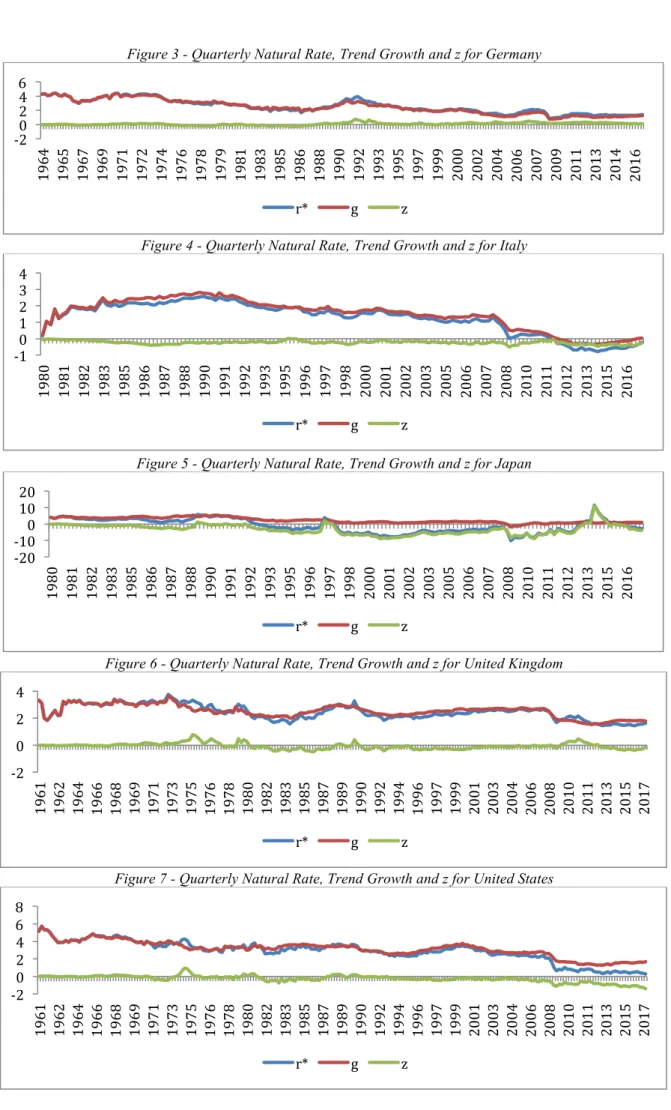
Figures 1-7 in Appendix 2 present the one-sided estimates of the natural rate of interest, trend growth and other determinants component for each economy.
Although estimates of the NRI differ across economies due to countries own idiosyncrasies, for all the economies it is possible to identify a sharp decline of the natural rate of interest after the GFC of 2007. For the majority of the countries, the decline of the NRI is mainly due to a drop in the trend growth rate of potential output. Adversely, in France, highly persistent factors seem to play an important role in determining the NRI, mainly after 2007, and in Japan the NRI also appears to be more affected by other determinants after 1990. Furthermore, it is worth mentioning that Germany, Italy and France belong to a monetary union with single currency since 1999, and thus fundamentals such as the NRI and trend growth of potential output are expected to be similar in these countries. While in France and in Italy the natural rate of interest has dropped to negative values after the Eurozone sovereign
debt crisis of 2012, in Germany the NRI and trend growth increase significantly after the reunification in 1990 and do not fall significantly after the global financial crisis, remaining at approximately 1%. In view of this, a single interest rate for the Euro area does not appear to be optimal.
The case for Japan is quite different. The natural rate of interest begins to decline and reaches negative values after the financial crisis in the 1990s. This negative trend is exacerbated during the financial crisis of 2007. Moreover, it is possible to observe that the NRI increases significantly in the first and second quarter of 2014, which can be explained by the increase in sales tax rate from 5% to 8% and, consequently, core consumer inflation increased to an all-time high over the past 30 years, nonetheless the NRI declines to negative values afterwards. All in all, it is possible to conclude that the natural rate of interest has been decreasing in G7 throughout the sample period, which is in accordance with the Secular Stagnation hypothesis and these findings are robust given that several studies reached similar conclusions.
4 THE EFFECT OF INEQUALITY ON THE NRI
4.1. Description of the ModelThe following equations show our benchmark model for the effect of inequality on the NRI and the additional control variables:
7 !∗= 1
! ! + ! + !
8 ! !"#$, !"#$%&'(ℎ!"#, !"#$%&' !"#$, !∗ = !(!"#$%&'(), !"#$%&, !"#$%&&'(, !∗)
9 !!,!∗ = !
!+ !!!"#$!,!+ !!!"!,!+ !!!"#"$%"$&'!,!+ +!!!"#$%"&'ℎ!,!+ !!!"#$%!"#$!,!
+ !!!"#$%&&'(!,!+ !!!"#$%&!,!+ !!!"#$%&"'()ℎ + !!,!
In Equation (7) the neoclassical Ramsey framework is depicted and links the equilibrium real rate with trend growth !, population growth, !, and shifts in preferences, !. With regard to trend growth of output, economic theory predicts a positive link between the former and the NRI. Furthermore, the link between population growth and the NRI is uncertain, however it is
argued that slower population growth reduces the marginal product of capital an consequently decreases the NRI. Additionally, given that the equilibrium real interest rate is the relative price of consumption, shifts in preferences !, which describes household consumption over their life cycle, play an important role in determining the NRI. Equation (8) shows the savings-investment (S-I) framework and is used to quantify how secular trends influence preference shifts and, consequently, the fluctuations of the NRI10. Lastly, equation (9) shows the reduced-form equation used to estimate the effect of inequality on the NRI, while controlling for other secular trends put forward in literature, trend growth and population growth. Equation (9) is then estimated using a fixed-effects11 model for an unbalanced panel of 7 countries from 1980 to 2016. This method is preferred over a Pooled OLS given that the former does not account for heterogeneity between countries, which can give rise to omitted variable bias. Additionally, fixed effects, unlike random effects, do not impose the strong assumption that country unobserved characteristics (e.g. cultural factors) are uncorrelated with the regressors, which is likely to be violated. Moreover, in order to account for cross-section dependence of the data, autocorrelation and heteroscedasticity of the residuals12, Driscoll-Kraay standard errors are deployed. The dependent variable of the model is the one-sided estimates of the NRI, which were previously estimated and annualized by taking the average of quarterly data from 1980 to 2016. Above all, we focus on the effects of wealth distribution (ineq). Our primary measure of inequality is the net Gini coefficient (post tax and transfers) ranging from 0 (total equality) to 100 (all income held by one person), which is taken from the version 6.0 of Standardized World Income Inequality Database (SWIID) by Frederic Solt (2016). Given that this coefficient is usually not directly comparable across
10 In the model, we study the effect of ex-post saving and investment, that is, the effect of savings and
investment secular trend on the NRI after taking into account investment and savings sensitivity and the
interplay between savings, investment and the NRI. Thus, the coefficients of the model will be downward biased
11 We perform the Hausman specification test and reject the null that random effects is preferred due to higher
efficiency in favor of the alternative that fixed effects is consistent
12 We concluded that the data exhibits cross-section dependence, heteroscedasticity and autocorrelation of the
residuals after performing the appropriate tests. Moreover, tests regarding the stationarity of the variables were performed and can be found in Table 3 in Appendix 1
countries due to different income definitions or accounting units, the SWIID uses a missing data multiple-imputation algorithm to standardized observations from various sources (Bofinger and Scheuermeyer, 2016). Besides that, we use total income share held by the richest top 10 percent collected from the World Income Database (WID). Wealth effects are measured via the ratio of net national wealth to net national income, which were derived by Piketty and Zucman (2014). Given that wealth tends to be highly concentrated due to cumulative processes governing wealth inequality dynamics, rising wealth-income ratios play a role for the overall structure of inequality. Furthermore, to isolate the true impact of inequality on the NRI, we control for other determinants of the natural rate of interest put forward such as demographics associated with stagnant population growth (PopGrowth) and dependency ratios (Dependency), the emerging markets savings glut hypothesis (CA), the difference between cost of capital and risk free rate using spread measured as a proxy (Spread), the declining relative price of capital goods (PInvGoods), falling productivity growth (TrendGrowth) and declining public investment (PublicInv). Detailed information regarding the variables description and sources is shown in Table 4 in Appendix 2.
4.2. Determinants of the Natural Rate of Interest
As it was previously mentioned, the NRI is determined by trend growth, population growth and other determinants shaping preferences for desired savings and investment. First of all, trend growth of potential output has been decreasing for all G7 countries mainly after the latest GFC, when there was a sharp drop and has still not returned to pre-crisis growth levels, nonetheless the slow pace of growth can only explain part of the secular decline of the NRI. Considering the S-I framework we have the following mechanism: An increase in savings puts downward pressures in the equilibrium real rate, whereas a decrease in investment will decrease the natural rate of interest.
Gross National Savings as a percentage of GDP (see Figure 8 in Appendix 2) has been increasing significantly after the global financial crisis and sovereign debt crisis of the Eurozone. Rachel and Smith (2015) argue that the increase in savings is due to the following secular trends: Rising inequality, emerging markets savings glut and demographics. With regard to demographics, economic theory predicts that there is a negative relationship between the dependency ratio and the savings rate since consumers prefer to smooth consumption over time and income is hump-shaped and thus the lower the proportion of dependents the higher will be the savings rate. In fact, in G7 countries there is a declining tendency of the young dependency ratio associated with the slowdown of population growth13. Furthermore, rising inequality increases savings and consequently decreases the real equilibrium interest rate based on the premise that the rich save more than the poor. For the majority of G7 countries net Gini has been increasing significantly, with the exception of France, however this trend dissipated after 2007 (see Figure 10-11 in Appendix 2).
Lastly, emerging markets such as Japan (see Figure 12 in Appendix 2) increased significantly their foreign exchange reserves since 1998 as a precautionary measure against capital outflows, which results in current account surpluses and in an increase in global savings commonly known as the emerging markets savings glut (Bernanke, 2005).
Considering the Investment Schedule, Figure 13 in Appendix 2 shows the sharp decline after the financial crisis of 2007 in investment as a percentage of GDP averaged for G7 countries. Rachel and Smith (2015) assert that this decline is mainly due to falling relative price of investment goods, a decline in public investment and a rise in the spread between the risk free rate and the cost of capital. First of all, the relative price of capital goods compared with consumption goods has been decreasing in G7 since 1980 (see Figure 14 in Appendix 2), however the effect of the relative price of investment goods is ambiguous since it depends on
13 The decline of the young dependency ratio does not appear to offset the rise of old dependents for G7 given
the elasticity between capital and labor. If the elasticity is equal or greater than one then the decline in the relative price of capital will induce additional investment projects by an amount that investment as a share of GDP doesn’t decline but given that most of the literature (e.g. Thwaites, 2015) conclude that the elasticity is smaller than one, Investment Schedule will shift to the left and, consequently, the NRI will decrease. Additionally, real public investment as a percentage of GDP has been decreasing in G7 countries (see Figure 15 in Appendix 2), which is mainly explained by the countries adjustment of the excessive levels of Debt to GDP. At last, given that the return on capital is what actually matters for investment decisions but the risk-free rate is the one used in the S-I framework, a rise in spread14 further reduces investment and the risk free rate. Given that there is no measure of spread between cost of capital and risk free rate, Rachel and Smith (2015) suggested credit spread, equity spread and fixed income spread15 to be used as proxies but given the insufficient data for earning yields and corporate bond yields for the G7, the former two weren’t calculated. Detailed information regarding the expected sign of the coefficient is shown in Table 5 in Appendix 1.
4.3. Empirical Results
Table 6 presents the results of the main model. Column (1) depicts the results from the estimation without any set of control variables. Column (2) includes the full set of control variables and in Column (3) we excluded total income held by the top 10% share. Consistent with the literature, our main variable of focus (net Gini) is negative and statistically significant for all alternative specifications. In Column (1) both net Gini and top 10% are positive and statistically significant, however net national wealth to income ratio is statistically significant. Furthermore, inequality appears to explain 27.44% of the time variation of the natural rate of interest. The inclusion of control variables in Column (2)
14 The rise in spread can be explained by the increasingly demand for safe assets that occurred after the Global Financial Crisis of 2007 and created a downward pressure in the rate of riskless assets
15 Credit Spread = lending – deposit bank rate; Equity Spread = earning yields – government bond yields; Fixed Income spread = corporate bond yields – government bond yields
increases significantly the explanatory power of the model and reduces the magnitude of the effect of inequality on the natural rate of interest. Interpreting our results, we see that an increase in net Gini by 1 percentage point (pp) reduces the natural rate by 0.1198 percent and the effect is significant at a 5% significance level. Notwithstanding, other measures of inequality are statistically insignificant. Column (3) reports the results from the estimation excluding top 10% share from the model given the possibility of multicollinearity between the three measures of inequality16. Another concern regarding this measure is the significant amount of missing values that may be nonrandom, which can lead to biased parameter estimates17. In this case, the effect of net Gini on the natural rate of interest is reduced (-0.073) but still significant at a 10% level. Even though net national wealth to income ratio is positive and statistically significant at a 10% level, the overall effect of inequality on the NRI could still be negative18. In sum, our findings suggest that rising inequality has contributed to the decrease in the time-varying NRI. Accordingly, the rich seem to save proportionally more than the poor, as opposed to what is suggested by the expenditure cascade proposition.
Regarding the control variables, it is worth mentioning that, in accordance with theoretical predictions, the coefficients of public investment, trend growth and the dependency ratio are positive and statistically significant in all specifications. Contrary to the literature, the coefficient of current account (CA) is positive and significant at 5% in Column (2) but loses its statistical significance in the estimation in Column (3). This can be explained by the fact that the majority of the countries from our sample are running current account deficits and only Japan is included in our sample to represent the emerging market savings glut hypothesis and thus it is poorly captured. At last, our results in Column (3) suggest that, contrary to previous studies, the relative price of capital is greater than 1, nonetheless this effect isn’t
16 For Further analysis regarding the correlation between variables see Table 7 in Appendix 1
17 This measure is subject to a variety of biases given issues related with sampling (underrepresentation of the
rich due to tax evasion) and problems regarding comparability between countries due to different income definitions and accounting units
significant for all specifications and thus the effect of the relative price of capital remains ambiguous.
Table 6 – Baseline Regressions
Notes: All regressions were estimated using fixed-effects with Driscoll-Kraay standard errors in parenthesis for the coefficients of interest. Significance levels: 1%*** 5%** 10%*
In addition, the within R2 reported in Column (2) implies that 83.65% of the amount of time variation of the natural rate of interest is explained by time variation in the explanatory variables. In fact, due to data constrains, we were unable to quantify other trends such as the spread between the risk free and cost of capital or short-termism19, which could explain why 16.35% of the time variation of the NRI is left unexplained.
4.4. Robustness
In this section, we test whether the relationship between inequality and the NRI is robust to variations in sample composition and by diving the sample between Euro countries and non-Euro countries. The results from the restricted sample and subsamples estimations are displayed in Table 8.
19 Excessive focus on short term results, which leads to an increase in future discounting
(1) (2) (3) Gini -0.446*** (0.1536) -0.1198** (0.051) -0.0734* (0.041) Top10 -0.109** (0.047) 0.0895 (0.061) - WealthInc 0.003 (0.003) 0.0013 (0.001) 0.0028* (0.001) CA - 0.0852** (0.034) 0.0445 (0.038) Dependency - 0.2708* (0.154) 0.3994*** (0.126) PopGrowth - -0.1022 (0.264) -0.3481 (0.219) PublicInv - 0.4626*** (0.141) 0.4297** (0.134) PInvGoods - -0.3197 (0.994) -1.678*** (0.508) CreditSpread - -0.0187 (0.040) -0.0497 (0.054) TrendGrowth - 2.0544*** (0.168) 2.045*** (0.162) Constant 18.11*** (3.247) -14.066** (5.391) -15.20*** (4.627) Observations 211 190 211 Countries 7 7 7 R2 0.2744 0.8365 0.8221
Table 8 – Restricted Country or Time Samples (1) 1980-2006 2007-2016 (2) Euro (3) Non-Euro (4) Gini -0.124*** (0.036) -1.140** (0.426) -0.0731 (0.064) -0.148** (0.059) WealthInc 0.0056*** (0.001) -0.001 (0.003) -0.002 (0.001) 0.006*** (0.002) CA 0.122*** (0.028) -0.094 (0.038) 0.022 (0.02) 0.0189 (0.053) Dependency 0.5523*** (0.101) 0.6032 (0.591) 0.261 (0.18) 0.5662*** (0.185) PopGrowth -0.449 (0.280) (0.591) -0.839 0.402*** (0.111) -1.186 (0.889) PublicInv 0.5746*** (0.105) -0.674* (0.328) -0.063 (0.134) 0.536*** (0.154) PInvGoods -1.468** (0.549) 1.008 (11.26) -2.845 (1.281) -1.518* (0.869) CreditSpread 0.0063 (0.026) 0.0028 (0.147) (0.038) 0.0005 (0.064) 0.0537 TrendGrowth 2.293*** (0.169) 1.889*** (0.177) 1.317*** (0.253) 2.079*** (0.17) Constant -21.61*** (4.074) 15.25** (10.06) (6.788) -3.599 (6.583) -21.17 Observations 161 40 91 120 Countries 7 6 3 4 R2 0.8518 0.7405 0.8149 0.841
Notes: All regressions were estimated using fixed-effects with Driscoll-Kraay standard errors in parenthesis for the coefficients of interest. Significance levels: 1%*** 5%** 10%*. Income held by the top 10% share was excluded from the estimation given the issues previously mentioned.
From Columns (1)-(2) it is possible to conclude that Gini is negative and statistically significant at 1% and 5% respectively, and that the negative effect of inequality on the time-varying natural rate of interest is magnified after the financial crisis of 2007. Column (3) includes only Euro members from our sample and net Gini becomes statistically insignificant with only trend growth and population growth being statistically significant at a 1% significance level. Nonetheless, we suspect that the results from this regression are subject to omitted variable bias. This is because when analyzing European countries one should take into account the ‘balance-sheet recession’ concept (Teulings and Baldwin, 2014). After the sovereign debt crisis of the Eurozone, governments paying down their debt resulted in an increase in savings that was not accompanied by a simultaneous increase in investment, which putted downward pressures in the NRI. To test this, we included general government debt to GDP as a control variable (see Table 9 in Appendix 1). In this case, net Gini becomes
statistically significant at 1% and debt to GDP is negative20 and statistically significant for Euro countries but insignificant for Non-euro countries. At last, in Column (4) it is possible to observe that inequality, proportion of dependents, price of capital goods, public investment and trend growth are important determinants of the NRI for countries outside the Euro. In addition, we test if the results are robust to alternative measures of the natural rate of interest (see Figures 16-22 in Appendix 2), which can be viewed in Table 10.
Table 10 – Alternative measures of the NRI (1)
HP Filter Ex-ante real rate (2) Two-sided estimates (3)
Gini 0.012 (0.06) (0.069) -0.028 (0.045) -0.023 WealthInc -0.011*** (0.001) -0.008*** (0.002) -0.003*** (0.001) CA -0.1059* (0.058) (0.062) -0.064 (0.016) 0.006 Dependency -0.814*** (0.229) -0.887*** (0.265) 0.042* (0.047) PopGrowth -0.226 (0.544) -0.041 (0.836) 0.503** (0.203) PublicInv -0.949 (0.279) -1.296*** (0.349) (0.105) 0.011 PInvGoods 3.826** (1.670) 5.87** (2.267) -1.11* (0.608) CreditSpread 0.051 (0.092) 0.134 (0.113) -0.077 (0.054) TrendGrowth 0.866** (0.273) 0.881 (0.343) 1.30*** (0.098) Constant -32.57*** (7.106) 33.78** (8.67) -0.604 (1.475) Observations 211 211 211 Countries 7 7 7 R2 0.6796 0.5556 0.8466
Notes: All regressions were estimated using fixed-effects with Driscoll-Kraay standard errors in parenthesis for the coefficients of interest. Significance levels: 1%*** 5%** 10%*. Income held by the top 10% share was excluded from the estimation given the issues mentioned previously.
Columns (1), (2) and (3) depict the results from the estimation using as the dependent variable the NRI estimated with univariate HP filter21 and the ex-ante real rate22 and two-sided (smoothed) estimates. For all of the alternative measures, the results change notably given that net Gini isn’t statistically significant and net wealth to income ratios appears to be a better predictor of the negative effect of inequality on the NRI. As it was previously mentioned, multivariate filters provide more accurate measures of the NRI given that they are able to capture information from inflation and output. Moreover, two-sided estimates are
20 Higher levels of debt require higher savings in order to stabilize or decrease the levels of debt
21 We used a ! of 6400 so that the HP filter estimates would capture the low frequency components as the
Kalman Filter
22 If monetary policy is set correctly then the real rate gap will be zero and the ex-ante real rate will be equal to
preferred to one-sided estimates23, however given that they are smoother, the time-variation in the NRI is reduced and so the model loses its statistical power. In light of this, conclusions regarding the causes of secular stagnation must be dealt carefully given that the dependent variable of our model is constructed based on certain economic and low frequency components behavior assumptions that may not be necessarily true.
5 CONCLUSIONS
This research investigates whether inequality has contributed to the decline in the time-varying natural rate of interest and, hence, its importance within the secular stagnation proposition. In a first step, this research applies the Laubach and Williams (2003) methodology to jointly estimate the natural rate of interest, output gap and trend growth of potential output for the G7. Our findings suggest that the NRI has been decreasing in all countries and suffered a sharp drop after the GFC of 2007. Accordingly, these findings corroborate the idea that we are living in the age of secular stagnation, however empirical evidence concerning the root of this problem remains scarce. Given the contagious malady proposition (Eggertsson et al, 2016) that, with financial openness, secular stagnation is a global phenomenon since it is transmitted between countries, it is crucial to understand the international trends placing downward pressures on the natural rate of interest. Thus, in a second step, we study the effect of trend growth, population growth and shifts in the S-I framework on the NRI, with rising inequality being our main focus by estimating fixed effects regressions using a panel of G7 members with unbalanced data from 1980 to 2016. Our findings suggest that, in accordance with economic theory, rising inequality is one of the main determinants of the decline in the time-varying NRI and that this negative effect of inequality is exacerbated after the GFC.
23 Two-sided estimates account for all the information, past and future, to estimate the NRI at time t, whereas
This paper entails data limitations arising from the reliability of inequality measures, which are associated with high measurement errors. What is more, our results might differ from some degree of omitted time-varying characteristics that we were unable to include in the set of control variables. Thus, an interesting extension to the present research could be to include these missing trends and to expand the set of countries used. For instance, by including emerging markets it would be possible to quantify the effect of the global savings glut on the NRI. At last, we tested the robustness of our results by using as the dependent variable the NRI estimated with HP filter, two-sided and ex-ante real rate and the results changed remarkably. In light of this, conclusions based on our model must be dealt carefully given that the dependent variable is subject to a high degree of uncertainty and our results aren’t robust to alternative methodologies used to estimate it. Thus, this paper calls for the further development of more accurate measures of the NRI.
REFERENCES
• Andrews, Donald, and Werner Ploberger. 1994. “Optimal Tests When a Nuisance Parameter is Present Only Under the Alternative.” Econometrica, 62: 1383-1414.
• Alvarez-Cuadrado, Francisco, and Mayssun El-Attar Vilalta. 2012. “Income inequality and saving”. Institute for the Study of Labor Discussion Paper 7083.
• Bernanke, Ben. 2005. “The Global saving glut and the U.S. current account deficit”, Paper presented at the Sandridge Lecture, Richmond, Virginia.
• Bofinger, Petter, and Philipp Scheuermeyer. 2016. “Income Distribution and Aggregate Saving: A Non-Monotonic Relationship”, CEPR Discussion Paper 11435.
• Cingano, Frederico. 2014. “Trends in Income Inequality and its Impact on Economic Growth.” Employment and Migration Working Paper 163.
• Clark, Todd E., and Sharon Kozicki. 2004. “Estimating Equilibrium Real Rates in Real-time.” Deutsche Bundesbank Discussion Paper 32.
• Cynamon, Barry Z., and Steven M. Fazzari. 2016. “Inequality, the Great Recession, and slow recovery.” Cambridge Journal of Economics 40(2): 373-399.
• Dynan, Karen E., Jonathan Skinner, and Stephen P. Zeldes. 2004. “Do the rich save more?” Journal of
Political Economy, 112(2): 397–444.
• Eggertsson, Gauti B. and Neil R. Mehrotra. 2014. “A Model of Secular Stagnation.” National Bureau of Economic Research Working Paper 20574.
• Eggertsson, Gauti B., Neil R. Mehrotra, Sanjay R. Singh & Lawrence H. Summers. 2016. “A Contagious Malady? Open Economy Dimensions of Secular Stagnation.” IMF Economic Review, 64(4): 581-634
• Frank, Robert H., Adam S. Levine, and Oege Dijk. 2014. “Expenditure cascades”, Review of
Behavioral Economics, 1 (12): 55-73.
• Garnier, Julien, and Bjorn-Roger Wilhelmsen. 2005. “The Natural Real Interest Rate and the Output Gap in the Euro Area: A joint estimation.” European Central Bank Working Paper Series 546.
• Giammarioli, Nicola, and Natacha Valla. 2003. “The Natural Real Rate of Interest in the Euro Area.” European Central Bank Working Paper 223
• Gordon, Robert J. 2015. “Secular Stagnation: A Supply-Side View.” American Economic Review, 105(5): 54-59.
• Hamilton, James D., Ethan S. Harris, Jan Hatzius, and Kenneth D. West. 2016. “The Equilibrium Real Funds Rate: Past, Present and Future.” International Monetary Fund Economic Review, 64(4): 660-707. • Holston, Kathryn, Thomas Laubach, and John C. Williams. 2016. “Measuring the Natural Rate of Interest: International Trends and Determinants.” Federal Reserve Bank of San Francisco Working Paper 2016-11.
• Keynes, John M. 1936. The General Theory of Employment, Interest and Money. New York: Harcourt Brace & Co
• Koo, Richard C. 2011. “The World in a Balance Sheet Recession: Causes, Cure and Politics.”
Real-World Economics Review, 58.
• Kuttner, Kenneth. 1994. “Estimating Potential Output as a Latent Variable.” Journal of Business and
Economic Statistics, 12(3): 361-368.
• Laubach, Thomas and John C.Williams. 2003. “Measuring the Natural Rate of Interest.” The Review of
Business and Economics and Statistics, 12(3): 361-368.
• Laubach, Thomas, and John C. Williams. 2015. “Measuring the Natural Rate of Interest Redux.”
Business Economics, 51: 257-267.
• Leigh, Andrew, and Albert Posso. 2009. ‘Top Incomes And National Savings’, Review of Income and
Wealth, 55(1): 57–74.
• Li, Hongyi, and Heng-fu Zou. 2004. “Savings and Income Distribution.” Annals of Economics and
Finance, 5(2): 245–270.
• Lubik, Thomas A., and Christian Matthes. 2015. “Calculating the Natural Rate of Interest: A Comparison of Two Alternative Approaches.” Federal Reserve Bank of Richmond Economic Brief 15-10.
• Mésonnier, Jean-Stéphane, and Jean-Paul Renne. 2007. “A Time-Varying Natural Rate of Interest for the Euro Area.” European Economic Review, 51: 1768-1784.
• Neiss, Katharine S., and Edward Nelson. 2001. “The Real Interest Rate Gap as an Inflation Indicator.” Centre for Economic Policy Research Discussion Paper 2848.
• Orphanides, Athanasios, and John C. Williams. 2002. “Robust Monetary Policy Rules with Unknown Natural Rates.” Federal Reserve Bank of San Francisco Working Paper 2003-01.
• Ostry, Jonathan D., Andrew Berg, and Charalambos G. Tsangarides. 2014. “Redistribution, Inequality and Growth.” International Monetary Fund Staff Discussion 14-02.
• Pescatori, Andrea and Jarkko Turunen. 2015. “Lower for Longer; Neutral Interest Rates in the United States.” International Monetary Fund Working Paper 2015-135.
• Rachel, Lukasz, and Thomas D Smith. 2015. “Secular Drivers of the Global Real Interest Rate.” Bank of England Staff Working Papers 571.
• Schmidt-Hebbel, Klaus, and Luis Servén. 2000. “Does income inequality raise aggregate saving?”
Journal of Development Economics, 61: 417–446.
• Smith, Douglas. 2001. “International Evidence on how Income inequality and credit market imperfections affect private saving rate.” Journal of Development Economics, 64(1): 103-127
• Stock, James H. 1994. “Unit Roots, Structural Breaks and Trends.” in R. Engle and D. Macfadden (eds)
‘Handbook of Econometrics,’ Vol. 4, Amsterdam, Elsevier Science, 2739-2841.
• Stock, James H., and Mark W. Watson. 1998. “Median Unbiased Estimation of Coefficient Variance in a Time-Varying Parameter Model.” Journal of the American Statistical Association, 93: 349-358. • Summers, Lawrence H. 2014. “US economic prospects: secular stagnation, hysteresis and the zero
lower bound” Business Economics 49(2): 65-73.
• Summers, Lawrence H. 2014. “Bold Reform is the only answer to secular stagnation,” Financial Times. 7 September.
• Summers, Lawrence H. 2014. “Reflections on the ‘New Secular Stagnation Hypothesis”, in Coen
Teulings and Richard Baldwin (eds) ‘Secular Stagnation: Facts, Causes and Cures’, Centre for Economic Policy Research Press: 27-40.
• Summers, Lawrence H. 2015. “Demand Side Secular Stagnation” American Economic Review, 105 (5), 60-65.
• Teulings, Coen, and Richard Baldwin. 2014. Secular Stagnation: Facts, Causes and Cures, London: Centre for Economic Policy Research Press: 27-40.
• Thwaites, Guy. 2015. “Why are real interest rates so low? Secular stagnation and the relative price of investment goods”, Centre for Macroeconomics Discussion Paper 2014-28.
• Wicksell, Knut. 1936. Interest and Prices, London: Macmillan.
• Wynne, Mark and Ren Zhang. 2017. “Estimating the Natural Rate in an Open Economy.” Globalization and Monetary Policy Institute Working Paper 316.
APPENDIX 1 – TABLES
Table 1 – HLW Estimation Variable Description
Interest Rates GDP Inflation
CA
Canada Bank Rate and after 2001 target rate from Canada Statistics
Website Real Gross Domestic Product, Seasonally Adjusted, Index from
IMF (IFS)
CPI used prior to 1984Q2 and core CPI from Canada
Statistics
US
NY discount Rate and Fed Funds
Rate from FRED Real Gross Domestic Product, Billions of Chained 2009 Dollars, Seasonally
Adjusted
Consumer Price index excluding food and energy
from FRED
GB
Monthly Official Bank Rate history from Bank of England Interactive
Statistical Database
ONS Website ABMI series: “Gross Domestic Product, Chained Volume Measures, Seasonally Adjusted, Millions of Pounds” CPI prior to 1970Q1 and Core
CPI from OECD
JP
BoJ Official Discount rate prior to 1986 and uncollateralized overnight
rate from bank of japan website
Real Gross Domestic Product, Seasonally Adjusted, Index from
IMF (IFS)
Consumer Price Index excluding food and energy
from OECD Statistics - Prices and Purchasing Power Parities FR
Short-term Interest Rates from OECD Data
Gross Domestic Product, US dollars, Constant Prices and PPPs, OECD base
year from OECD National Accounts
Statistics IT
Table 2 – HLW Estimation Parameters Parameter CA FR DE IT JP GB US Sample 1961Q1 – 2017Q1 1972Q1 – 2017Q2 1964Q1 – 2017Q2 1980Q1 – 2017Q2 1980Q1 – 2017Q2 1961Q1 – 2017Q2 1961Q1 – 2017Q2 !! 0.043 0.022 0.056 0.042 0.089 0.025 0.052 !! 0.015 0.056 0.010 0.027 0.018 0.022 0.032 !!+ !! 0.952 0.959 0.919 0.899 0.332 0.915 0.942 !! -0.060 -0.036 -0.070 -0.043 -0.003 -0.008 -0.070 (t-stat) (3.01) (2.75) (1.70) (1.64) (0.09) (1.70) (4.06) !! 0.075 0.077 0.133 0.105 1.839 0.562 0.077 (t-stat) (2.07) (1.63) (1.86) (1.97) (1.16) (2.14) (3.09) !! 0.345 0.218 0.717 0.281 0.299 0.104 0.355 !! 1.764 1.132 1.131 1.158 0.973 2.929 0.792 !! 0.638 0.349 0.593 0.517 0.912 0.872 0.571 !! 1.122 0.425 1.013 0.928 1.428 0.456 0.119 !! 0.092 0.818 0.176 0.104 1.655 0.233 0.161 !! = !!!+ ! !! 1.126 0.922 1.029 0.934 3.128 0.512 0.200 S.E. (sample average) !∗ 1.196 2.838 2.259 2.619 4.726 3.123 1.114 ! 0.413 0.187 0.450 0.328 0.804 0.416 0.395 !∗ 2.079 1.626 1.509 1.221 0.341 0.834 1.534 S.E. (final observation) !∗ 1.632 4.415 3.254 3.731 6.099 4.491 1.600 ! 0.556 0.253 0.635 0.434 0.537 0.549 0.541 !∗ 2.508 2.639 2.068 1.313 0.373 0.938 2.054
Table 3 – Augmented Dicker-Fuller Unit Root Test, Test Statistics Variable CA FR DE IT JP GB US Natural Rate -3.22* -1.43 -3.64** -3.01 -2.37 -3.18* -2.35 (First Difference) -6.22*** -5.4*** -5.4*** -4.8*** -5.0*** -6.8*** -6.11*** Trend Growth -3.27* -2.26 -3.54*** -3.2* -2.06 -3.81*** -2.48 (First Difference) -6.49*** -5.7*** -5.43*** -4.0*** -5.1*** -6.1*** -6.54*** CA -2.16 -1.92 -2.16 -2.86 -3.44** -2.73 -2.75 (First Difference) -3.39* -4.18** -2.74 -4.38*** -5.63*** -4.56*** -4.01** Dependency -3.70** -2.17 -2.11 -2.54 -0.78 -3.20* -3.51** (First Difference) -1.77 -2.08 -2.93 -1.72 -2.28 -1.59 -2.09 PopGrowth -2.18 -2.80 -2.75 -1.64 -1.94 -1.74 -1.99 (First Difference) -5.89*** -4.93*** -3.48* -3.24* -4.09** -4.91 -3.82** PublicInv -1.69 -2.98 -1.43 -2.06 -2.22 -2.26 -2.59 (First Difference) -3.42** -3.77** -5.88*** -4.39*** -3.54** -3.35* -3.10 Spread -2.18 -2.34 -1.68 -2.85 -3.45* -3.79** -1.89 (First Difference) -3.71** -4.43*** -2.03 -6.27*** -4.02** -6.37*** -2.71 PInvGoods -1.61 -1.61 -0.75 -2.08 -2.47 -2.25 -1.37 (First Difference) -3.62** -3.57** -2.23 -2.29 -7.01*** -3.43* -5.05*** Top10 -1.74 -2.01 (Missing values) (Missing values) -3.13 (Missing values) -2.39 (First Difference) -4.97** -3.49* (Missing values) (Missing values) -4.06** (Missing values) -4.11** WealthInc -0.19 -2.01 -2.80 -3.74** -1.09 -2.72 -3.44* (First Difference) -3.06 -2.41 -3.53** -4.41*** -3.75** -4.29*** -5.74*** Gini -2.87 -1.69 -1.37 -2.07 -1.48 -2.34 -2.39 (First Difference) -2.49 -2.56 -2.44 -3.26* -0.56 -1.70 -3.01
Notes: * Represents that the null hypothesis of a unit root can be rejected with 10% level of
significance and ** represents that it can be rejected with a 5% level of significance and *** represents that it can be rejected with a 1% level of significance.
Table 4 – Variable Description
Variable Description Mean (Std.
Dev.)
Min Max. Obs Source
Natural Rate of
Interest Real Interest Rate consistent with stable inflation and output
1.54 (2.08) -8.5 6.35 259 LW Estimation
Net Gini Coefficient Gini (0 to 100) adjusted for tax and transfers
30.89 (3.18) 24.2 37.8 249 SWIID 6.0.
Top 10% Pre-tax National Income
(Labor + Capital Income) held by the richest 10%
36.45 (4.73) 26.0 47.1 211 World Income Database Wealth to Income
Ratio Net National Wealth to Net National Income 459 (112) 260 803 250 World Income Database Current Account Current Account Balances as
a percentage of GDP
-0.22 (2.78) -5.8 8.58 259 OECD Economic Outlook 2017 Dependency
Ratio Dependents (<15 and >65) as a percentage of working age population
32.90 (2.43) 23.4 37.9 239 OECD Statistics – Demography and
Population Population Growth Annual changes in population
resulting from births, deaths and net migration
0.51 (0.45) 0.45 -0.91 240 OECD Statistics – Demography and
Population Relative Price of
Investment Goods (GCF) deflator/ Final Private Gross Capital Formation Consumption Expenditure Deflator 1.07 (0.12) 0.93 1.56 248 OECD Economic Outlook 2017 – GDP Deflators and Forecast Growth Public Investment General Government Gross
Fixed Capital Formation (GFC) as a percentage of GDP (in Billions of constant
2011 international dollars)
3.99 (1.77) 1.59 10.7 252 IMF Investment and Capital Stock Dataset, 2017
Credit Spread Bank Credit Spread = Lending Rate – Deposit Rate
3.62 (1.77) -1.3 10.2 238 World Bank via IMF (IFS)
Trend Growth Growth Rate of Potential Output – output reached when
the economy is at full employment
Table 5 – Economic Predictions of the effect of the variables on the NRI Variable Effect CA ∂r ∗ ∂CA< 0 → CA ↑→ S ↑→ r ∗↓ Gini ∂r ∗ ∂Gini< 0 → Gini ↑→ S ↑→ r ∗↓ Dependency Ratio ∂r ∗ ∂Dependency> 0 → YoungDep ↑→ S ↓→ r ∗↑ TrendGrowth ∂r ∗ ∂TrendGrowth> 0 → TrendGrowth ↑→ r ∗↑ PublicInv ∂r ∗ ∂PublicInv> 0 → PublicInv ↑→ I ↑→ r ∗↑ Spread ∂r ∗ ∂Spread1< 0 → Spread1 ↑→ r ∗↓ PopGrowth* ∂r ∗ ∂PopGrowth> 0 → r ∗↑ Top10 ∂r ∗ ∂Top10< 0 → Top10 ↑→ S ↑→ r ∗↓ WealthInc ∂r ∗ ∂WealthInc< 0 → WealthInc ↑→ S ↑→ r ∗↓ PInvGoods* ∂r ∗ ∂PInvGoods> 0 → PcapitalGoods ↑→ I ↑→ r ∗↑
Notes: * represents ambiguity regarding the sign of the coefficients for population growth and the
relative price of investment goods
Table 7 – Correlation Matrix
r* Gini T10 W/I Dep PopG PubInv PInvG Spread g CA r* 1.00 Gini -0.01 1.00 T10 -0.11 0.449 1.00 W/I -0.51 0.043 0.15 1.00 Dep -0.17 0.394 0.02 0.08 1.00 PopG 0.36 0.255 0.36 -0.22 0.00 1.00 PubInv -0.29 -0.24 -0.06 0.54 -0.10 0.07 1.00 PInvG 0.321 0.063 -0.19 -0.18 0.17 -0.07 -0.09 1.00 Spread 0.239 -0.18 -0.55 -0.23 -0.29 -0.15 -0.20 -0.188 1.00 g 0.675 -0.16 -0.05 -0.26 -0.21 0.42 0.237 0.359 0.09 1.00 CA -0.313 -0.50 -0.15 0.16 -0.19 -0.50 0.183 -0.253 -0.03 -0.24 1.00