Automatic numerical solution of elasticity problems by a local mesh-free multi-objective optimization framework

AUTOMATIC NUMERICAL SOLUTION OF ELASTICITY PROBLEMS BY A LOCAL

MESH-FREE MULTI-OBJECTIVE OPTIMIZATION FRAMEWORK

WILBER HUMBERTO VÉLEZ GÓMEZ

DOCTOR THESIS IN STRUCTURES AND CIVIL CONSTRUCTION

DEPARTMENT OF ENVIRONMENTAL AND CIVIL ENGINEERING

FACULTY OF TECHNOLOGY

UNIVERSITY OF BRASÍLIA

FACULTY OF TECHNOLOGY

DEPARTMENT OF ENVIRONMENTAL AND CIVIL ENGINEERING

AUTOMATIC NUMERICAL SOLUTION OF ELASTICITY

PROBLEMS BY A LOCAL MESH-FREE MULTI-OBJECTIVE

OPTIMIZATION FRAMEWORK

WILBER HUMBERTO VÉLEZ GÓMEZ

SUPERVISOR: ARTUR ANTÓNIO DE ALMEIDA PORTELA, PhD.

UNIVERSITY OF BRASÍLIA

FACULTY OF TECHNOLOGY

DEPARTMENT OF ENVIRONMENTAL AND CIVIL ENGINEERING

NUMERICAL SOLUTION OF ELASTICITY PROBLEMS BY A LOCAL

MESH-FREE MULTI-OBJECTIVE OPTIMIZATION FRAMEWORK

WILBER HUMBERTO VÉLEZ GÓMEZ

DOCTOR THESIS SUBMITTED TO THE DEPARTMENT OF

ENVIRONMENTAL AND CIVIL ENGINEERING OF THE FACULTY OF

TECHNOLOGY OF THE UNIVERSITY OF BRASÍLIA AS PART OF

THE REQUIREMENTS REQUIRED FOR OBTAINING THE DOCTOR

DEGREE IN STRUCTURES AND CIVIL CONSTRUCTION.

APPROVED BY:

Prof. Artur António de Almeida Portela, PhD. (ENC-UnB)

(Supervisor)

Prof. Luciano Mendez Bezerra, PhD. (ENC-UnB)

(Internal examiner)

Prof. Luis Alejandro Perez Peña, PhD. (FAU-UnB)

(External examiner)

Prof. Luiz Carlos Wrobel, PhD. (CIV-PUC RIO)

(External examiner)

3.Optimização Multi-Objetivo 4.Algoritmo genetico

II.Título (Doutor) 1.Método sem malha local

2.Teorema do Trabalho Local I.ENC/FT/UnB

GÓMEZ, WILBER HUMBERTO VÉLEZ

Numerical solution of elasticity problems by a local mesh-free multi-objective optimization method [Distrito Federal] 2019.

xx, 100p., 210 x 297 mm (ENC/FT/UnB, Doutor, Estruturas e Construção Civil, 2019). Tese de doutorado – Universidade de Brasília. Faculdade de Tecnologia.

Departamento de Engenharia Civil e Ambiental. FICHA CATALOGRÁFICA

REFERÊNCIA BIBLIOGRÁFICA

GÓMEZ, W. H. V. (2019). Numerical solution of elasticity problems by a local mesh-free multi-objetive optimization framework. Tese de doutorado em Estruturas e Construção Civil, Publicação E.TD-14A/19, Departamento de Engenharia Civil e Ambiental, Universidade de Brasília, Brasília, DF, 100p.

CESSÃO DE DIREITOS

AUTOR: Wilber Humberto Vélez Gómez.

TÍTULO: Numerical solution of elasticity problems by a local mesh-free multi-objetive optimization framework.

GRAU: Doutor ANO: 2019

É concedida à Universidade de Brasília permissão para reproduzir cópias desta dissertação de mestrado e para emprestar ou vender tais cópias somente para propósitos acadêmicos e científicos. O autor reserva outros direitos de publicação e nenhuma parte dessa dissertação de mestrado pode ser reproduzida sem autorização por escrito do autor.

Wilber Humberto Vélez Gómez SHC/N CL QD. 406 BL B, Asa Norte 70.847-520. Brasília – DF – Brasil. wilbervelez@hotmail.com

Acknowledgments

First of all I’d to thank God for helping me in this great and important project, opening paths and allowing me to meet wonderful people who made this great adventure so much better. I thank my family, my parents Genny Gomez and Humberto Velez, my sisters Julieth and Claudia and my nephew Samuel Osorio. Also, my grandmother, uncles and cousins. Thank you all for your support and encouragement on this journey.

The CNPQ for the economic support. To the professors of the Graduate Program in Structures and Construction at the University of Brasilia (UnB) for the new learning and the opportunity to acquire new experiences. To my advisor Artur Portela for his help, dedication and motivation, my Mesh-free UnB friends Tiago, Flavio, Elvis, Fernando, Amanda and Thiago.

My gratitude to all the staff of UnB employees who contribute daily so that we can develop our research. I am very grateful to those who have done this work best for their help and friendship. Iarly, Gabriel, Jerfson, Henrique, Pedro, Luciano (lulu), Nasser, Rodolfo, Thiago, Nataniel, Gelson, Wilson, Juliana, Renan, Amir Mahdi, Matheus, Ana, Mara, Divino, Erica, Myrelle, Wilson, Nathaly, Jaime, Daniela, Pipe, Yuri, John Kennedy, and others who have supported me from before with their company Jader, Cristina, Leydi and Damaris.

To the brothers Enilton and Eliana Victor who accepted me at their home as part of the family, the Gravina family for their company and great help in this process, the and the other friends and brothers of the Assembleia de Deus of Brasilia.

But we have this wealth in vessels of earth, so that it may be seen that the power comes not from us but from God. Troubles are round us on every side, but we are not shut in; things are hard for us, but we see a way out of them. We are cruelly attacked, but not without hope; we are made low, but we are not without help. II Corinthians 4: 7 - 9

AUTOMATIC NUMERICAL SOLUTION OF ELASTICITY PROBLEMS

BY A LOCAL MESH-FREE MULTI-OBJECTIVE OPTIMIZATION

FRAMEWORK

Author: Wilber Humberto Vélez Gómez Supervisor: Artur António de Almeida Portela

Postgraduate Program in Structures and Civil Construction Brasília, December 6, 2019

ABSTRACT

Project automation, whatever its nature, is a highly relevant study, as it generally speeds up the processes involved by increasing productivity. Regarding structural design automation, a common problem is the discretization used in structural element analysis by numerical methods. Thus, the automation of this process brings great advantages and increased productivity in accomplishing this task. Since the automatic use of the optimization of the numerical analysis is always fast and highly accurate, without the need for user intervention, facilitating the execution of structural design.

The concern of this work is the numerical solution of two-dimensional problems of linear elasticity, carried out with an automatic implementation of a mesh free numerical analysis, through a multi-objective optimization process. The goal of this automation strategy of analysis is to simultaneously improving the accuracy, efficiency, stability, and conditioning of the numerical solver of the mesh free method, with minimal effort of the designer. The mesh free method is based in a local formulation and therefore, uses a node-by-node process to generate the global system of equilibrium equations of a nodal discretization. Furthermore, in the local domain of integration of each node, the respective equilibrium equations are generated with a reduced numerical integration, which improves the accuracy of results. The novelty of the thesis is the complete automation of the mesh free numerical analysis. Hence, the location coordinates and the sizes of, respectively the compact support and the local integration domain, of each node of the discretization, are automatically defined by means of a robust evolutionary multi-objective optimization process, based on genetic algorithms. Benchmark problems were analyzed to assess the accuracy and efficiency of presented techniques. The results shown in this work are in perfect agreement with those of

analytical solutions and thus, make quite reliable this strategy of automatic local mesh free numerical analysis, carried out with a multi-objective optimization process.

Keywords: Local formulation; Local mesh-free method; Reduced numerical integration; Multi-objective optimization; Genetic algorithms.

SOLUÇÃO NUMÉRICA AUTOMÁTICA DE PROBLEMAS DE

ELASTICIDADE COM OTIMIZAÇÃO MULTI-OBJETIVO DE

METODOS SEM MALHA LOCAIS

Orientador: Artur António de Almeida Portela

Programa de Pos-graduação em Estruturas e Construção Civil Brasília, 6 de Dezembro, 2019

RESUMO

A automação de projetos, seja ele de qualquer natureza, é um estudo altamente relevante, visto que de maneira geral ela acelera os processos envolvidos aumentando a produtividade. A respeito da automação de projetos estruturais, um problema comum é a discretização usadas na análise de elemento estruturais por via de métodos numéricos. Dessa maneira, a automação desse processo traz grandes vantagens e aumento da produtividade na realização dessa tarefa. Visto que, o uso automático da otimização da análise numérica, é sempre rápida e altamente precisa, sem a necessidade de intervenção do usuário, facilitando a execução do projeto estrutural.

O objetivo deste trabalho é a solução numérica de problemas bidimensionais de elasticidade linear. Para isso, é realizada a implementação automática de uma análise numérica sem malha, através de um processo multiobjetivo de otimização. O objetivo desta estratégia de análise de automação é melhorar simultaneamente a precisão, eficiência, estabilidade e condicionamento do solucionador numérico do método sem malha, com o mínimo esforço do projetista. O método sem malha é baseado em uma formulação local e, portanto, utiliza um processo nó por nó para gerar o sistema global de equações de equilíbrio de uma discretização nodal. Além disso, no domínio local de integração de cada nó, as respectivas equações de equilíbrio são geradas com uma integração numérica reduzida, o que melhora a precisão dos resultados.

A novidade da tese é a automação completa da análise numérica sem malha. Portanto, as coordenadas de localização e o tamanho do suporte compacto e o domínio de integração local, de cada nó da discretização, são definidos automaticamente por meio de um processo robusto e otimizado por funções multiobjetivo, baseado em algoritmos genéticos. Problemas de benchmark foram analisados para avaliar a precisão e eficiência das técnicas apresentadas. Os resultados apresentados neste trabalho estão em perfeita concordância com os das soluções analíticas e, portanto, tornam bastante confiável essa estratégia de análise numérica automática de métodos sem malha local, realizada com um processo de otimização multiobjetivo.

Palavras chave: Formulação local; Método sem malha local; Integração númerica reduzida; Optimização Multi-objectivo; Algoritmo genetico.

CONTENTS

LIST OF FIGURES xvi

LIST OF SYMBOLS, NOMENCLATURES AND ABBREVIATIONS xvii

1 INTRODUCTION 1 1.1 MOTIVATION . . . 2 1.2 OBJECTIVES . . . . 3 1.2.1 General objective . . . 3 1.2.2 Specific objectives . . . 3 1.3 THESIS LAYOUT . . . 4 2 LITERATURE REVIEW 5 2.1 MESHFREE METHOD . . . . 5

2.1.1 Local Meshfree Method . . . 6

2.2 REDUCED INTEGRATION . . . 7

2.3 NUMERICAL OPTIMIZATION . . . . 8

3 STRUCTURAL MODELING 10 3.1 LOCAL DOMAIN . . . 11

3.2 THE WORK THEOREM . . . 11

3.3 KINEMATIC FORMULATIONS . . . . 12

3.3.1 Rigid-body displacement formulation . . . 13

3.3.2 Mechanical equilibrium . . . . 13

3.4 MODELING STRATEGY . . . . 13

3.4.1 Defining the strain field . . . 14

3.4.2 Defining the stress field . . . 14

4 LOCAL MESH-FREE NUMERICAL METHOD 16 4.1 REDUCED INTEGRATION FORMULATION . . . 19

4.2 PARAMETERS OF LOCAL MESH-FREE METHOD . . . . 21

5 OPTIMIZATION WHIT GENETIC ALGORITHMS 23 5.1 Multi-objective Optimization Problem . . . . 23

5.1.1 Feasible Set . . . 23

5.1.2 Pareto Dominance . . . . 24

5.1.3 Pareto Optimality . . . 24

5.2 Genetic Algorithms Search and Decision Making ... 25

5.2.1 Objective Functions of the ILMF Model ... 26

5.2.2 Formulation and implmentation ... 28

6 NUMERICAL RESULTS 32 6.1 CANTILEVER-BEAM ... 32

6.1.1 Performance of the reduced integration of ILMF ... 33

6.1.2 Influence of the local compact support domain size (αs) and the local integration domain size (αq) ... 36

6.1.3 Irregular nodal distributions ... 40

6.1.4 Automatic Discretization ... 45

6.2 CIRCULAR CYLINDER ... 55

6.2.1 Internal pressure ... 55

6.2.2 External pressure ... 60

6.3 PLATE WITH A CIRCULAR HOLE... 66

6.4 OBJETIVE FUNCTIONS ... 72 7 CONCLUSIONS 74 7.1 GENERAL CONCLUSIONS ... 74 7.2 FUTURE WORKS ... 75 REFERENCES 80 ANNEXES 81 A MLS APPROXIMATION 82 A.1 SHAPE FUNCTIONS... 82

A.2 WEIGHT FUNCTIONS ... 84

A.3 ELASTIC FIELD ... 85

B COMPARISON WITH OTHER NUMERICAL METHODS 86 B.1 CANTILEVER BEAM ... 86

B.2 CIRCULAR CYLINDER WITH INTERNAL PRESSURE... 88

B.3 CIRCULAR CYLINDER WITH EXTERNAL PRESSURE... 90

B.4 PLATE WITH A CIRCULAR HOLE... 92

C MATLAB 95 C.1 SPECIFYING GA OPTIONS ... 95

D LOCAL MESH-FREE METHOD OPTIMIZATION WITH GENETIC ALGORITMS AND ARTIFICIAL NEURAL NETWORKS 97

E PAPERS AND INTERNATIONAL CONFERENCES 99 E.1 PAPERS ... 99 E.2 INTERNATIONAL CONFERENCES ... 99

LIST OF FIGURES

3.1 Representation of the body’s domain Ω, with boundary Γ = Γu ∪ Γt; the work theorem is defined in an arbitrary domain ΩQ ∈ Ω ∪ Γ, assigned to a reference point Q ∈ ΩQ, with boundary ΓQ = ΓQi ∪ΓQt ∪ΓQu, in which ΓQi is the interior local boundary, and ΓQt and ΓQu are local boundaries that share the global boundaries, respectively the static boundary Γt and the kinematic boundary Γu; points P and R, have arbitrary local domains, respectively ΩP and ΩR ... 10 3.2 Schematic representation of the work theorem, an energy relationship, valid

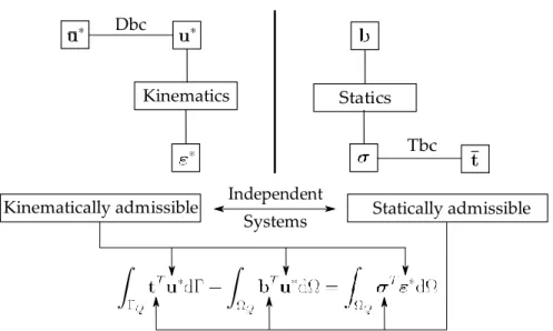
in an arbitrary local domain ΩQ ∈ Ω ∪ Γ, with boundary ΓQ, between any two independent fields, in which one of them, the stress field σ, is required to satisfy equilibrium with a system of external forces b and t, while the other, the strain field ε∗, is required to satisfy compatibility with a set of constrained displacements u∗, in the domain Ω ∪ Γ of the body ... 12 3.3 Modeling strategy of kinematic models of the work theorem. After choosing the

kinematically admissible strain field, the strategy considers that the statically admissible stress field is always assumed as the stress field of the unique elastic field that actually settles in the body which satisfies full admissibility. Dbc and Tbc stands for Displacement boundary condition and Traction boundary condition respectively ... 14 4.1 Mesh free discretization of the domain Ω and boundary Γ = Γu ∪ Γt; reference

nodes P , Q and R have associated local domains ΩP , ΩQ and ΩR; the local domain ΩQ, assigned to the node Q, where the work theorem is defined, has boundary ΓQ = ΓQi ∪ ΓQt ∪ ΓQu, in which ΓQi is the interior local boundary

and ΓQt ∈ Γt and ΓQu ∈ Γu ... 16 4.2 Schematic representation of a mesh-free discretization of the global domain Ω

and boundary Γ, with a distribution of nodes; ΩP , ΩQ and ΩR represent the local compact supports of the corresponding nodes xP , xQ and xR; Ωx is the

domain of definition, of the MLS approximation of the sampling point x, which is the set of nodes, in this case xP , xQ and xR, whose compact support contains this sampling point. ... 17 4.3 Schematic representation of numerical-quadrature points, on each side, or

quadrant, of local domains, for the computation of the local form of the work

4.4 Schematic representation of rectangular and circular local domains, with 1 collocation point on each side, or quadrant, of the local domain, for the computation of the generalized local form of the work theorem, with the

rigid-body displacement formulation. ... 20

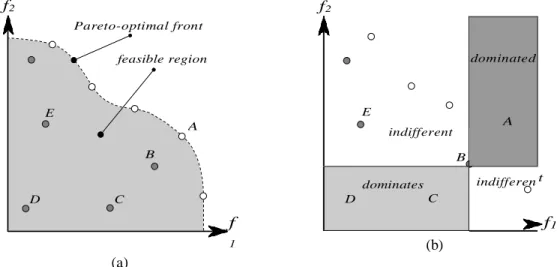
5.1 Representation of Pareto optimality in objective space, on the left (a), and the possible relations of solutions in objective space, on the right (b). ... 24

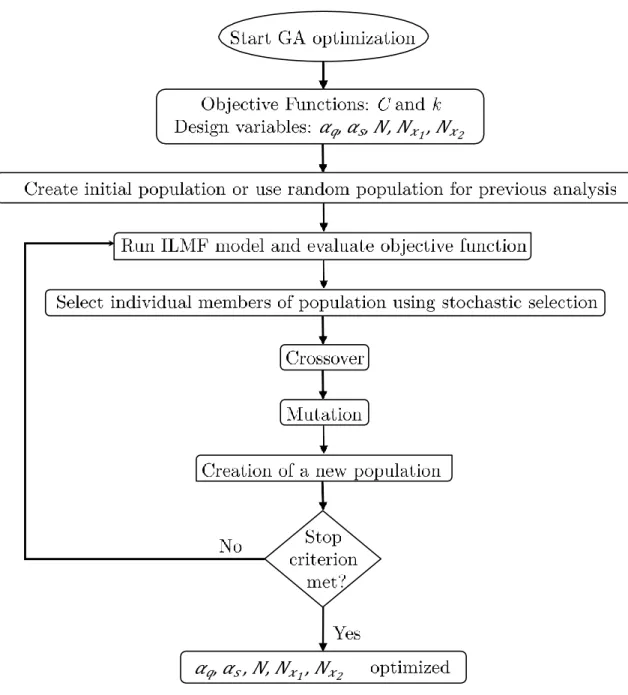
5.2 Flowchart of the routine defined for the mono-objective optimization. ... 30

5.3 Floowchart of the routine defined for the Multi-objective Optimization. ... 31

6.1 Timoshenko cantilever beam. ... 33

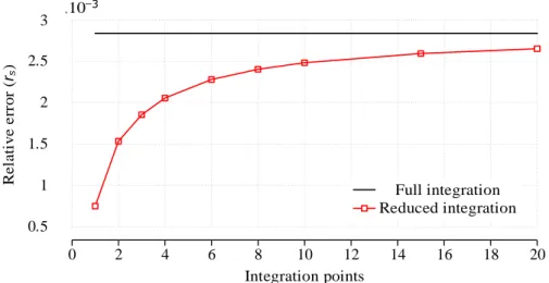
6.2 ILMF energy relative error (rs), as a function of the number of equally-spaced integration points, for a regular distribution of 33 × 5 = 165 nodes; results of MLPG, obtained with 10 points per segment of the local domain, referred to as full integration. ... 34

6.3 ILMF energy relative error (rs), for the beam discretization with 52, 165, 585, 1261 and 2193 nodes, as a function of the equally-spaced integration points, on the boundaries of the respective local domain. ... 35

6.4 ILMF relative error rs, for the beam discretization with 13 × 4 = 52, 33 × 5 = 165 and 65×9 = 585 nodes, as a function of the number of nodes, considering a complete set of 1st and 2nd order polynomial basis for the MLS approximation. As expected, the ILMF accuracy increases with finer nodal distributions and higher order polynomial basis. ... 36

6.5 Analysis of influence of the local compact support domain size on Energy relative error (rε), Compliance (C) and Condition number (k), carried out for three discretization with 13 × 4 = 52, 33 × 5 = 165 and 65 × 9 = 585 nodes, and αq = 0.5. ... 38

6.6 Analysis of influence of the local compact support domain size on Energy relative error (rε), Compliance (C) and Condition number (k), carried out for three discretization with 13 × 4 = 52, 33 × 5 = 165 and 65 × 9 = 585 nodes, and αq = 0.5. ... 39

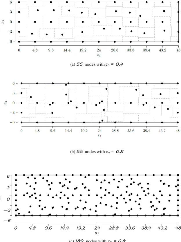
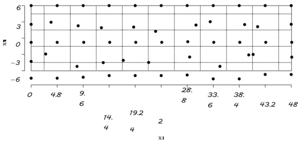
6.7 Nodal distributions of the beam discretization with 189 nodes and level-1 of irregularity; in configuration A, only interior nodes have an irregular distribution, as presented by Liu (2003), while in configuration B all nodes are irregularly distributed. ... 41

6.8 ILMF energy relative error, computed with αq = 0.5, as a function of the irregularity parameter cn, obtained with irregular nodal distributions with 55, 189, 561 and 697 nodes of the beam discretization. The ILMF accuracy is evident. 42 6.9 Nodal distributions of the beam discretization, with 55 and 189 nodes with irregularity of level-2 of interior nodes only ... 43

6.10 Energy relative error of ILMF and MLPG, as presented by Liu (2003), as a function of the irregularity parameter cn, obtained with irregular nodal

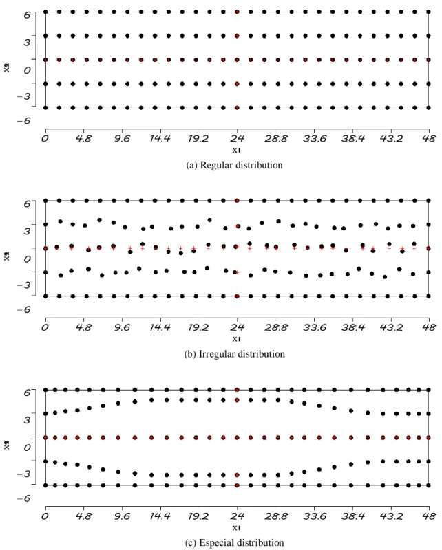
distributions of the beam discretization. The ILMF accuracy is evident. ... 44 6.11 Three different nodal distributions of the beam with 29×5 = 145 nodes with

irregularity of level-2 and Configuration A. ... 46 6.12 Principal displacement and stress for the cantilever beam with three different

nodal distribution. ... 47 6.13 Nodal distributions of the cantilever beam, discretization (5×11 = 55, and

41×17 = 697 nodes) with level-1 of irregularity in configuration A. ... 49 6.14 Energy relative error of ILMF and MLPG as a function of the irregularity

parameter cn, obtained for the irregular discretization of the cantilever beam. ... 49 6.15 The multi-objective Pareto front for irregular distribution of the cantilever beam

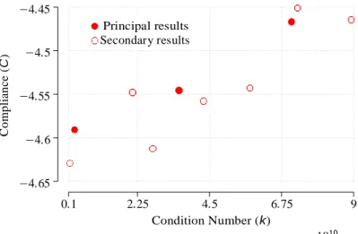
discretization, obtained with the automatic optimization routine. ... 50 6.16 Condition number (k) and Compliance (C) as a function of the number of nodes

(N ), carried out for three different optimization discretization of cantilever beam. 51 6.17 Nodal distributions of the cantilever beam, discretization (5×4 = 20, 9×5 = 45

and 15×9 = 135 nodes) with level-2 of irregularity; in configuration A. ... 52 6.18 Principal displacement and stress for the cantilever beam with three different

irregular nodal discretization, obtained by the automatic optimization routine. ... 53 6.19 Nodal distributions of the beam discretization with 20, 45 and 135 nodes with

level-2 of irregularity; in configuration A. ... 54 6.20 Circular cylinder with internal and external pressure. ... 55 6.21 Circular cylinder with internal pressure. ... 56 6.22 The multi-objective Pareto front for irregular distribution of the circular cylinder

discretizations with internal pressure, obtained with the automatic optimization routine. ... 56 6.23 Condition number (k) and Compliance (C) as a function of the number of

nodes (N ), carried out for three different optimization discretizations of circular cylinder with internal pressure... 57 6.24 Nodal distributions of the circular cylinder with external pressure, discretization

(8×6 = 48, 11×8 = 88 and 17×11 = 187 nodes) with level-2 of irregularity; in configuration A. ... 58 6.25 Principal displacement and stress for the circular cylinder with internal pressure

carried out for three different irregular nodal discretizations, obtained by the

automatic optimization routine. ... 59 6.26 Analysis of the influence of the number of nodes (N ) on Condition number (k)

and Compliance (C), carried out for three different optimization discretization. 60 6.27 Circular cylinder with internal pressure. ... 60

6.28 The multi-objective Pareto front for irregular distribution of the circular cyliner discretization with external pressure, obtained with the automatic optimization routine. ... 61 6.29 Condition number (k) and Compliance (C) as a function of the number of

nodes (N ), carried out for three different optimization discretization of circular cylinder with external pressure. ... 62 6.30 Nodal distributions of the circular cylinder with external pressure, discretization

(8×7 = 56, 11×8 = 88 and 19×12 = 228 nodes) with level-2 of irregularity; in configuration A. ... 63 6.31 Principal displacement and stress for the circular cylinder with external pressure

carried out for three different irregular nodal discretization, obtained by the

automatic optimization routine. ... 64 6.32 Analysis of influence of the number of nodes (N ) on Condition number (k) and

Compliance (C), carried out for three different optimization discretization. ... 65 6.33 Plate with a circular hole. ... 66 6.34 The multi-objective Pareto front for irregular distribution of the plate with a

circular hole discretization, obtained with the automatic optimization routine. ... 67 6.35 Condition number (k) and Compliance (C) as a function of the number of

nodes (N ), carried out for three different optimization discretization of plate with circular hole. ... 68 6.36 Nodal distributions of the plate with a circular hole, discretization (12×7 = 84,

15×9 = 135 and 19×13 = 247 nodes) with level-2 of irregularity; in

configuration A. ... 69 6.37 Horizontal and vertical displacement of the plate with a circular hole, carried

out for three different irregular nodal discretization, obtained by the automatic optimization routine. ... 70 6.38 Stress distribution of the plate with circular hole for θ = 0, π/4, π/2, carried

out for three different irregular nodal discretizations, obtained by the automatic optimization routine. ... 71 6.39 Energy and displacement relative errors as a function of the number of nodes,

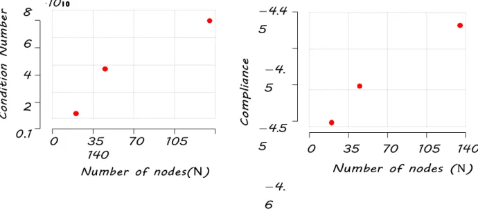
carried out for three different optimization discretizations of plate with circular hole. ... 72 6.40 Condition number (k) as a function of the number of nodes (N ), carried out for

different benchmark problems with automatic discretization. ... 72 6.41 Compliance (C) as a function of the number of nodes (N ), carried out for

different benchmark problems with automatic discretization. ... 73 A.1 Schematic representation of the MLS approximation in one dimension. ... 82

A.2 Typical weight function and shape function of the MLS approximation for a node at x = [1/2 0]T ... 83 B.1 Nodal distributions of the cantilever beam, discretization with 15×9 = 135

nodes and level-2 of irregularity; in configuration A. ... 86 B.2 Principal displacement and stress for the cantilever beam with three different

numerical methods. ... 87 B.3 Nodal distributions of the circular cylinder with external pressure, discretization

with 17×11 = 187 nodes and level-2 of irregularity; in configuration A. ... 88 B.4 Principal displacement and stress for the circular cylinder with internal pressure

carried out for three different numerical methods. ... 89 B.5 Nodal distributions of the circular cylinder with external pressure, discretization

with 19×12 = 228 nodes and level-2 of irregularity; in configuration A. ... 90 B.6 Principal displacement and stress for the circular cylinder with external pressure

carried out for three different irregular nodal discretization, obtained by the

automatic optimization routine. ... 91 B.7 Nodal distributions of the plate with a circular hole, discretization 19×13 = 247

nodes and level-2 of irregularity; in configuration A. ... 92 B.8 Horizontal and vertical displacement of the plate with a circular hole, carried

out for three different numerical methods. ... 93 B.9 Stress distribution of the plate with circular hole for θ = 0, π/4, π/2, carried

out for three different numerical methods. ... 94 D.1 Nodal distributions of the beam discretization with 189 nodes and level-1 of

irregularity; in configuration A, only interior nodes have an irregular distribution, as presented by Liu (2003), while in configuration B all nodes are irregularly distributed. ... 98

LIST OF SYMBOLS, NOMENCLATURES AND ABBREVIATIONS

Abbreviations

ANN Artificial Neural Networks CAD Computer Aided Design

Dbc Displacement boundary condition DEM Diffuse Element Method

EFG Element Free Galerkin FEM Finite Element Method GA Genetic Algorithms

GFEM Generalized Finite Element Method

ILMF Local Mesh-Free Method whit reduced integration LMFM Local Mesh-Free Method

LPIM Local Point Interpolation Method

LRPIM Local Radial Point Interpolation Method MLBIE Mesh-Free Local Boundary Integral Equation MLPG Mesh-Free Local Petrov-Galerkin

MLS Moving least Squares

PSO Particle Swarm Optimization

PUFEM Partition of Unity Finite Element Method RKPM Reproducing Kernel Particle Method SA Simulated Annealing

SOS Symbiotic Organisms Search SPH Smoothed Particle Hydrodynamics Tbc Traction boundary condition

Greek Alphabet Symbols (r, θ) Polar coordinates

αq Parameter size of the local integration domain αs Parameter size of the compact support domain

ε Strain field

ε∗ _{Kinematecally-admissible strain field}

Γ Global domain boundary

ΓQi Interior local boundary associated with the node Q ΓQ Local boundary associated with the node Q

Γt Static boundary Γu Kinematic boundary ǁεǁ Error energy norm ν PoissonJs ratio Ω Global domain

Ωx Definition domain of MLS approximation of the sampling point x ΩP Local compact support associated with the node xP

ΩQ Local compact support associated with the node xQ ΩR Local compact support associated with the node xR Φ Shape functions matrix

φ(i) Shape function of the MLS approximation for a node i σ Statically-admissible stress field

Latin Alphabet Symbols

uˆ Unknown nodal parameters ǁuǁ Error displacement norm

KQ Nodal stiffness matrix associated with the field node Q xi Spatial coordinate of the node i

a Dimension radius Ai Constant

b Dimension modeled section of the plate with a circular hole Bi Constant

C Compliance

Ci Distance of the node i to the nearest neighbouring node cn Parameter of nodal irregularity

D Depth cantilever beam d Distance function E Young’s modulus H(d) Heaviside step function I Moment of inertia k Condition Number L Length cantilever beam N Number of nodes P Shear force

S Area S of local domain ΩQ

w(i) Weight function of the MLS approximation for a node i B Matrix of linear operators

b Body forces c Vector constant K Vector global forces

n Matrix of the components of the unit outward normal t Vector of the tration components

u Displacements

WΓ Arbitrary weight function defined in Γ

WΩ Arbitrary weight function defined in Ω

t Vector of the prescribed tractions

u∗ _{Strain field generated by continuos displacements}

1 - INTRODUCTION

Mesh free numerical methods achieved a remarkable progress over the past few years. The essential feature of these methods is that they perform the discretization of the problem domain and boundaries with a set of scattered field nodes that do not require any mesh for the approximation of the field variables. Historically, most of published mesh free methods rely on background cells for the integration of the weighted residual weak form over the global domain, in the process of the generation of the system of algebraic equations and therefore, they cannot be considered truly mesh free methods.

Local mesh free methods, based on weighted residual local weak forms, have been developed to avoid the background mesh generation in cells. The most popular of these methods is the Meshless Local Petrov-Galerkin (MLPG) method, that is based on the well known moving least- squares (MLS) approximation. The main feature of this method is that local weak forms are used for integration on regular-shaped local regions instead of global weak forms and therefore, the method does not require to use a global background mesh, but only a local background mesh.

The accuracy and efficiency of local mesh free methods is determined by two discretization parameters. They are, respectively the size of the local compact support domain (αs) of each node, that is primarily linked to the accuracy of the model through the total number of nodes used to build the shape functions of the local node stiffness and, the size of the local integration domain (αq) of each node where the work theorem is numerically integrated, that is primarily linked to the efficiency of the model.

The optimization problem of mesh free discretization parameters involves two different sorts of difficulty, which are multiple conflicting objectives and a highly complex search space. In the first case, competing goals give rise to a set of compromise solutions known as Pareto- optimal, and none of the corresponding trade-offs can be said to be better than the others, when preference information is not available. Effectively, all these trade-off solutions are optimal in the wider sense that, in the search space, no other solutions are superior to them, when all objectives are taken into consideration. In the second case, the amplitude and complexity of the search space can be too large to be solved by classic exact methods. Consequently, efficient optimization strategies that are able to address both of these difficulties are required, in an effective way. Evolutionary algorithms have several attributes that are convenient for this sort of problem which, therefore, make them more suitable than classical optimization methods. Evolutionary approaches operate on a set of candidate solutions. Using strong simplifications,

this set is subsequently modified by basic operations based on the principles of evolution: selection, crossover and mutation. Genetic algorithms, which are a class of evolutionary methodologies, implement elitist strategy selection, which ensures that the individual with highest fitness is always copied into the next generation. Among these basic operations, the most important is crossover, because it plays a fundamental role in guiding the population toward an acceptable solution. In general, mutation is not considered to be an especially important operation and it is usually set at a very low rate, sometimes omitted, as reported by Eberhart and Shi (2007). In evolutionary algorithms, natural selection can be simulated by a stochastic selection process. Evolutionary algorithms are especially suited to multi-objective optimization because they can capture multiple Pareto-optimal solutions in a single simulation run and may exploit similarities of solutions by recombination.

This work is concerned with the implementation of the ILMF local mesh free method, presented by Oliveira et al. (2019), with automatic multi-objective optimization of the mesh free discretization parameters, using GA, for the solution automatic discretization of problems in two-dimensional linear elasticity.

1.1 - MOTIVATION

The discretization of the αs and αq parameters determine the accuracy and efficiency of the numerical method and therefore play a key role in the modeling strategy. Both parameters are usually arbitrarily defined and can vary depending on the local mesh free method used. The effect on accuracy and convergence of different parameters was studied by Moussaoui and Bouziane (2013) for the MLPG. The main drawback of dealing with heuristically defined discretization parameters is that their definition is not unique, and consequently cannot be easily implemented into an automatic procedure.

Therefore, an optimization attempt, using genetic algorithms (GA), was performed, on MLPG, by Baradaran and Mahmoodabadi (2009) for two dimensional steady-state heat conduction problems and by Bagheri et al. (2011) for three dimensional elastostatic problems. A similar optimization was proposed by Ebrahimnejad et al. (2015), combined with an additional adaptive refinement technique. Although these authors were successful, their attempt led to a very time consuming approach that requires an analytical solution to be performed and therefore is not efficient.

Thus, there is a clear need for an alternative modeling strategy that considers the implementation of automatic local mesh free numerical methods, with discretization parameter optimization and nodal configuration, without use of the analytical solution.

1.2 - OBJECTIVES

1.2.1 - General objective

The major objective of this thesis is the implementation of the automatic discretization of the new local mesh-free numerical method (ILMF), for solving two-dimensional problems in linear elastostatics. The formulation is derived with the work theorem, of the theory of structures, which turns out to be the weak form of a weighted-residual statement of a statically admissible stress field. The discretization is carried out locally, through a reduced numerical integration, which therefore generates the system of algebraic equations in a node by node scheme. The axiomatization of the discretization is performed in a multi-objective optimization framework of robust evolutionary methods based on genetic algorithms.

1.2.2 - Specific objectives

• Develop a local form of the work theorem, valid in an arbitrary local region of the structural body, to be applied in the formulation of a local mesh-free method, in the set of kinematically- admissible strain fields.

• Formulate and implement a local mesh-free method, with reduced integration, in the set of kinematically-admissible strain fields. Assess the virtues of both the formulation and the implementation of the reduced numerical integration, of the numerical method.

• Formulate and implement a local mesh-free method, with numerical reduced integration, for regular and irregular nodal discretization. Assess the behavior of the numerical method for both cases of the regular and irregular nodal distributions

• Formulate the multi-objective optimization process of the discretization. Define and assess the performance of the objective functions of the formulation.

• Formulate and implement the MATLAB genetic algorithms for the multi-objective optimization of both the nodal discretization and the dimensionless discretization parameters (αs and αq) of the local mesh-free method. Discuss the implementation.

• Compare the performance and efficiency of the automatic local mesh-free method developed, against other local mesh-free methods and available analytical solutions.

1.3 - THESIS LAYOUT

This thesis is developed in seven chapters. In chapter 1, introduction, the motivation, general and specific objectives are presented. Chapter 2, presents the literature review. Chapter 3, presents the theoretical and mathematical development of the local form of the work theorem, the local kinematic formulation for the rigid body displacement and modeling strategy. Chapter 4 presents the local mesh-free method. Chapter 5 presents the optimization of local mesh-free parameters. Chapter 6 presents some numerical results, obtained for a benchmark problem, which give evidence of the accuracy, efficiency and robustness of the strategies adopted for the automatic optimization process. Chapter 7 presents the conclusions and future ideas for research. Finally, complementary annexes used in this research are presented.

2 - LITERATURE REVIEW

One of the paths that were followed in the development of rational mechanics is based on the so-called principle of virtual works, already known, albeit in rudimentary form, by Aristotle and to which Galileo, later on, recognized generality for the first time. Connected with Lagrangian and Hamiltonian mechanics, the principle of the virtual works is a global principle linked to the concepts of work and energy. In the framework of the modern theory of structures, the virtual- work principle is no more than a particular case of the work theorem that is used as a generator of generalized models, as presented by Oliveira (1973).

The work theorem has been postulated as a unifying basis in the formulation of numerical methods in continuum mechanics, as early reported by Portela (1981) and Brebbia (1985). The work theorem establishes an energy relationship between a statically-admissible stress field and an independent kinematically-admissible strain field. The independence of these stress and strain fields is a key feature of the work theorem that allows the generation of different numerical methods. Recently, the local form of the work theorem, valid in an arbitrary local region of the structural body, was applied in the formulation of local mesh-free numerical methods, in the set of kinematically-admissible strain fields, as reported by Oliveira and Portela (2016).

2.1 - MESHFREE METHOD

Mesh-free numerical methods achieved a remarkable progress over the past few years. The essential feature of these methods is that they perform the discretization of the problem domain and boundaries with a set of scattered field nodes that do not require any mesh for the approximation of the field variables. In general, their formulation is based in the weighted-residual method presented by Finalyson (1972). In this work it is shown that the weak form, of the weighted-residual statement of a statically-admissible stress field, is obviously the work theorem of the theory of structures.

Smoothed particle hydrodynamics (SPH), presented by Lucy (1977) and Gingold and Monaghan (1977) is one of the earliest mesh-free methods applied to solve problems in astrophysics. Libersky et al. (1993) were the first to apply SPH in solid mechanics. The main drawbacks of SPH are inaccurate results near boundaries and tension instability that was first investigated by Swegle et al. (1995). SPH is based on a strong-form formulation of the weighted-residual method, with a Lagrangian description.

The collocation method is also based in the weighted-residual strong-form formulation. Typical mesh-free collocation methods were published by Sekher and Vinay (1997), Wu (1992), Zhang et al. (2001), Liu et al. (2002b), Onate et al. (1996), Lee and Yoon (2004) and Jamil and Ng (2013). Collocation methods have some attractive advantages over other mesh-free methods, as they implement a simple algorithm, with no integration required. Despite these advantages, collocation methods tend to be inaccurate and unstable, due to the ill-conditioned system equations. Onate et al. (2001) presented a stabilization technique suitable only for some particular problems.

Other mesh-free methods are based on a weighted-residual weak-form formulation. After discretization, the weak form is used to derive a system of algebraic equations, through a process of numerical integration, using background cells constructed in the domain of the problem. Research on these formulations significantly increased after the publication, by Nayroles et al. (1992), of the diffuse element method (DEM). The reproducing kernel particle method (RKPM), presented by Liu et al. (1995), and the element-free Galerkin (EFG) method, presented by Belytschko et al. (1994), were the first weak-form mesh-free methods applied in solid mechanics. In contrast to EFG and RKPM methods, with a so-called intrinsic basis, other methods with an extrinsic basis and the partition of unity concept were developed. This extrinsic basis was used in the hp-cloud method, presented by Duarte and Oden (1996). Melenk and Babuska (1996) presented the partition of unity finite element method (PUFEM) which is similar to the hp-cloud method; while PUFEM shape functions are based on Lagrange polynomials, the general form of the hp-cloud method also includes the MLS-approximation. Strouboulis et al. (2000) presented the generalized finite element method (GFEM) and pointed out that different partition of unities can be used for the usual approximation and the enrichment.

2.1.1 - Local Meshfree Method

All these weak-form mesh-free methods require the use of a background mesh for integration of the weighted-residual weak form over the global problem domain, and therefore, they are not truly mesh-free methods. To overcome this difficulty, a class of mesh-free methods based on local weighted-residual weak forms, such as the mesh-free local Petrov-Galerkin (MLPG) method presented by Atluri and Zhu (1988) to Atluri and Shen (2002), the mesh-free local boundary integral equation (MLBIE) method presented by Zhu et al. (1998), the local point interpolation method (LPIM) presented by Liu et al. (2001) and the local radial point interpolation method (LRPIM) presented by Liu et al. (2002a), have been developed. The main difference of the popular MLPG method to other global mesh-free methods, such as EFG or RKPM, is that local weak forms are used in MLPG, for integration on local domains, rather than global weak forms and consequently the method does not require the use of a background

global mesh, but only a background local grid. Note that, in contrast to the MLPG method, the new formulations presented in this work, which use generalized local weak forms, are completely free of integration, a very important feature when it comes to computational efficiency.

Local mesh-free methods exhibit excellent performance, at least in some particular applications. Despite of their performance, local mesh-free methods have not succeeded in replacing the standard displacement-assumed finite-element method (FEM), in general applications. It is well known that the global formulation of the standard FEM considers an element-by-element stiffness calculation that is assembled into the global stiffness matrix. This method of generating the final system of equations is not suitable for the analysis processing in parallel environments. Regarding this case, there is a clear advantage in using local formulations of FEM which consider a node-by-node stiffness calculation, to generate the respective rows of the global stiffness matrix. Therefore, the analysis processing can easily be parallelized, in terms of nodes, due to the independence of the nodal equations. Furthermore, the independence of the nodal equations allows, in local formulations of FEM, using of enrichment of a particular nodal stiffness matrix without increasing the nodal degrees of freedom.

2.2 - REDUCED INTEGRATION

The issue of numerical stability is quite significant when developing numerical methods. In the standard FEM, elements with a reduced number of integration points are routinely employed because they are computationally very effective and avoid locking problems of fully integrated elements. As a side effect, such reduced integrated elements are susceptible to spurious singular modes, so-called hourglass modes, which are zero-energy modes in the sense that the element deforms without an associated increase of the elastic energy. These spurious modes, generated by a reduced number of integration points, can be prevented through stabilization techniques. Zienkiewicz and Taylor (1983) and Bathe (2014) provide additional information on this concept. The reduced integration is the main source of the numerical instability of some meshfree methods, leading to unstable hourglass deformation and zero-energy modes. This is the case of the element-free Galerkin method, see Beissel and Belytschko (1996), and the meshfree particle method, as reported by Belytschko et al. (2000). Nodal integration, in meshfree methods without stabilization, leads to instabilities due to the fact that each node is associated with a support domain, where integrations are carried out, to compute the nodal stiffness. This implies that each integration domain is associated with only one integration point, that is the node and hence, when only one integration point is considered for higher order functions, other than constant strain, the nodal integration causes instabilities. In contrast, the new integrated numerical methods presented in this work consider, in the case of the meshfree

method, a total of 4 integration points to compute the stiffness associated to each local node which, therefore, prevents the generation of spurious zero-energy modes, unlike nodal integration methods without stabilization. In order to overcome solution instabilities that are present in direct nodal integration, Taylor series expansions have been used, to serve as stabilization terms, as presented, respectively by Liu et al. (1985), for FEM, and by Liu et al. (1996) and Liu et al. (2007), for meshfree methods. While stable, the drawback of this stabilization technique is that it requires the calculation of high order derivatives.

Therefore, there is still a clear need for an alternative modeling strategy that completely avoids all the issues associated with nodal integration. To fulfill such need, this work presents a linearly integrated local meshfree numerical method.

2.3 - NUMERICAL OPTIMIZATION

Optimization is the process of adjusting the input data or characteristics of a particular system, mathematical process, or experiment, thereby seeking to find the minimum or maximum output data, whether or not is the final result Haupt and Haupt (2004). Engineering problem solving involves multi-stage decision making. The main goal of all these decisions is to minimize the effort required or maximize the desired benefit, as seen in Rao (2009). Since the required effort or desired benefit in any practical situation can be expressed as a function of certain decision variables, optimization can be defined as the process of finding the condition that determines the maximum or minimum value of a function.

Several techniques have been developed over the years to solve different types of optimization problems. Mathematical programming techniques, also known as optimal solution search methods, are good at finding the minimum of a multi-variable function under a set of constraints. Stochastic process techniques can be used to analyze problems described by a set of random variables in a probability distribution. Finally, statistical methods allow the analysis of experimental data and the construction of empirical models, thus seeking to obtain the most accurate representation of the physical situation Goldberg and Holland (1988).

There are several ways to classify optimization problems. Whether or not there are restrictions, they can be classified as restricted or unrestricted. Regarding the nature of decision variables, they can be classified into two broad categories: first as a parameter or static optimization, second as a trajectory or dynamic optimization. Classifications between linear, nonlinear, geometric, and quadratic problems can be assigned with respect to the nature of expressions for the objective function and constraints. Based on the allowed values for decision variables, they can be classified as integers or actual values. Regarding the deterministic nature of the variables, the optimization problem can be classified as deterministic or stochastic. As for the

separation between objective functions and constraints, it can be classified as separable and non-separable. Finally, depending on the number of objective functions to be minimized, the problem and optimization can be classified as mono-objective and multi-objective, as seen in Rao (2009).

Recently, algorithms emerged with great results, including Genetic Algorithm (GA) developed by Holland (1975), Simulated Annealing (SA), developed by Kirkpatrick et al. (1983), Particle Swarm Optimization (PSO), presented by Parsopoulos and Vrahatis (2002). Adaptive Symbiotic Organisms Search developed by Tejani et al. (2016). These evolutionary methods generate new points in search space by applying operators to current points and moving statistically to optimal locations in space. The great results are the result of an intelligent search in a large but finite solution space using statistical methods.

Classic optimization methods are great at finding a single solution in just one interaction, thus making them inconvenient for problem solving with multiple objective functions. In contrast, as demonstrated by Deb (2001), evolutionary algorithms can find many optimal solutions, thanks to their sample space search process, particularly the mutation and the crossover. Thus, these methods are ideal for applications related to multi-objective problems, such as problems related to the present research.

∪ ∪ ∈ ∪ ∈ ∪

3 - STRUCTURAL MODELING

Consider the domain Ω of a body with boundary Γ subdivided in Γu and Γt, with Γ = Γu ∪ Γt, as Figure 3.1 represents.

Figure 3.1 – Representation of the body’s domain Ω, with boundary Γ = Γu Γt; the work theorem is defined in an arbitrary domain ΩQ Ω Γ, assigned to a reference point Q ΩQ, with boundary ΓQ = ΓQi ΓQt ΓQu, in which ΓQi is the interior local boundary, and ΓQt and ΓQu are local boundaries that share the global boundaries, respectively the static boundary Γt and the kinematic boundary Γu; points P and R, have arbitrary local domains, respectively ΩP

and ΩR.

The fundamental boundary value problem of elasticity aims to find, in Ω, the distribution of stresses σ, strains ε and displacements u, when it has displacements u, constrained on Γu, and is under the action of an external system of distributed surface and body forces with densities represented, respectively by t, on Γt and b, in Ω.

The solution of the posed problem, simultaneously satisfying kinematic admissibility of the strains and static admissibility of the stresses, is thus a fully admissible elastic field. Kirchhoff’s theorem, see Kirchhoff (1859), on the uniqueness of solutions of the elasticity boundary value problem shows that this solution is unique, assuming that it exists. The general work theorem will be used to solve the posed problem.

In the body’s domain, loaded by a system of external forces in the conditions already referred, consider a statically admissible stress field σ, which therefore satisfies

∫ ∫ ∫ in Ω, with boundary conditions

t = n σ = t, (3.2)

specified on Γt; L is a matrix differential operator; t denotes traction components; t denotes prescribed tractions and n is the matrix of the components of the unit normal to the boundary outwardly directed.

3.1 - LOCAL DOMAIN

In the body, consider an arbitrary local domain ΩQ ∈ Ω ∪ Γ, assigned to a reference point Q ∈ ΩQ, with boundary ΓQ = ΓQi ∪ΓQt ∪ΓQu, in which ΓQi is the interior local boundary, with local boundaries ΓQt and ΓQu sharing the global boundaries, respectively the static boundary Γt and the kinematic boundary Γu, as Figure 3.1 represents. The work theorem will be derived for this arbitrary local domain ΩQ. Due to its arbitrariness, this local domain ΩQ ∪ ΓQ ∈ Ω ∪ Γ can be overlapping with other similar sub-domains that can be defined in the body.

3.2 - THE WORK THEOREM

The work theorem, presented in Oliveira and Portela (2016), establishes an energy relationship, in an arbitrary local domain ΩQ ∈ Ω, between two independent elastic fields that can be defined in the body which are, respectively a statically admissible stress field σ that satisfies equilibrium with a system of external forces, and a kinematically admissible strain field ε∗ that satisfies compatibility with a set of constrained displacements. Expressed as an integral form, defined in the domain ΩQ ∪ ΓQ, the theorem of work can be written in a compact way, simply as

tT _u∗ _{dΓ +}

ΓQ ΩQ

bT _u∗ _{dΩ =}

ΩQ

σT _ε∗ _{dΩ, (3.3)}

in which no constitutive relation links the stress σ and the strain ε∗ and therefore, they do not depend on each other, as Figure 3.2 schematically represents.

The stress σ, a statically admissible field, can be any one that is in equilibrium with the system of external forces, therefore satisfying equations (3.1) and (3.2); it is not necessarily the stress that the system of external forces actually introduces in the body.

The strain ε∗, a kinematically admissible field, can be any one, generated by continuous displacements u∗ with small derivatives, compatible with an arbitrary set of constraints specified on the kinematic boundary; it is not necessarily the strain actually settled in the body.

∈ ∪

Independent Systems

Figure 3.2 – Schematic representation of the work theorem, an energy relationship, valid in an arbitrary local domain ΩQ Ω Γ, with boundary ΓQ, between any two independent fields, in

which one of them, the stress field σ, is required to satisfy equilibrium with a system of external forces b and t, while the other, the strain field ε∗, is required to satisfy compatibility

with a set of constrained displacements u∗, in the domain Ω ∪ Γ of the body.

Finally, the local domain ΩQ ∪ ΓQ is an arbitrary sub-domain of the body, associated with the reference point Q, as represented in Figure 3.1, where the independent fields σ and ε∗ are defined.

3.3 - KINEMATIC FORMULATIONS

In order to use the work theorem, as the starting point in the formulation of numerical methods, it is necessary to specify one of the two independent fields that can be defined in the body, in accordance with some particular convenience of the numerical method formulation.

Kinematic formulations consider a particular specification of the strain field ε∗, leading thus to an equation of mechanical equilibrium that is used in numerical models, to generate the respective stiffness matrix. A simple case of a kinematic formulation, based on a strain field generated by a rigid-body displacement.

Statics Dbc Kinematics Tbc Statically admissible Kinematically admissible

∫ ∫ ∫ 3.3.1 - Rigid-body displacement formulation

Bearing in mind the key feature of the work theorem, that is the complete independence of the admissible fields, σ and ε∗, the strain field is defined to simplify the formulation. Hence, the simplest and obvious choice is to use a strain field generated by a rigid-body displacement that can be defined as

u∗_{(x) = c, (3.4)}

in which c is a constant vector that conveniently generates null strains

ε∗_{(x) = 0. (3.5)}

The great virtue of this formulation is the simplicity used in the generation of the strain field; in addition, this formulation leads to a simple form of equilibrium equations that, in the absence of body forces, has no domain terms.

3.3.2 - Mechanical equilibrium

When the rigid-body displacement formulation is considered, the work theorem, equation (3.3), simply leads to the equation

ΓQ−ΓQt t dΓ + ΓQt t dΓ + ΩQ b dΩ = 0 (3.6)

which states an integral form of mechanical equilibrium, of tractions and body forces, in the domain ΩQ. Obviously, this equation expresses the local version of the Euler-Cauchy stress principle.

Local equilibrium equation (3.6), is used to generate the stiffness matrix associated to the local node.

3.4 - MODELING STRATEGY

The formulation of numerical methods can be based on the work theorem, along with a proper and convenient kinematic formulation, in order to derive the equilibrium equations that are used to generate the stiffness matrix of each numerical model. This modeling strategy is adopted to solve the actual elastic problem.

Kinematics

Constitutiveness Tbc

3.4.1 - Defining the strain field

The work theorem is kinematically formulated through the specification of an appropriate strain field ε∗. This thesis considers the arbitrary rigid-body displacement, to kinematically formulate the work theorem, thus leading to the equilibrium equation (3.6).

3.4.2 - Defining the stress field

This stage of the modeling strategy regards the definition of the statically admissible stress field, in the equilibrium equation (3.6). The stress field σ, required to satisfy equilibrium with a system of external forces, is assumed as the state of stress that actually settles in the body, loaded by the actual system of distributed surface and body forces, with the actual displacement constraints. This key assumption is schematically represented in Figure 3.3.

Independent Systems

Figure 3.3 – Modeling strategy of kinematic models of the work theorem. After choosing the kinematically admissible strain field, the strategy considers that the statically admissible stress

field is always assumed as the stress field of the unique elastic field that actually settles in the body which satisfies full admissibility. Dbc and Tbc stands for Displacement boundary

condition and Traction boundary condition respectively.

Recall that the elastic field that settles in the body is the unique fully admissible elastic field satisfying the given problem. Therefore, besides satisfying equilibrium, through equations (3.1) and (3.2), or through equation (3.6), generated by the work theorem, this unique fully admissible field also must satisfy compatibility, defined as

ε = L u, (3.7)

Dbc

Statics Dbc

Kinematics

Totally (kinematecally + statically) admissible Kinematically admissible

in Ω, with boundary conditions

u = u, (3.8)

on Γu, in which continuous displacements are assumed with small derivatives, leading to geometrical linearity of the strain field. Hence, equation (3.8), which specifies the constraints of the actual displacements, must be applied in any numerical model, in order to allow for a unique solution of the problem.

This thesis considers the absence of body forces in the formulation of the local mesh free method.

∪

4 - LOCAL MESH-FREE NUMERICAL METHOD

The essential feature of mesh free methods is that they perform the discretization of the problem only with a set of scattered nodes, without using any mesh for the approximation of the variables. The local mesh free method, presented in this paper, is based on the widely used approximation of the moving least-squares (MLS). The basic MLS terminology, introduced by Atluri and Zhu (2000), is presented here, along with a summary of the essential features of the MLS approximation, used in this work.

Each node of the mesh free discretization is associated with its local domain, as schematically represented in Figure 4.1. In general, this local domain is a circular or rectangular region,

Figure 4.1 – Mesh free discretization of the domain Ω and boundary Γ = Γu Γt; reference nodes P , Q and R have associated local domains ΩP , ΩQ and ΩR; the local domain ΩQ,

assigned to the node Q, where the work theorem is defined, has boundary

ΓQ = ΓQi ∪ ΓQt ∪ ΓQu, in which ΓQi is the interior local boundary and ΓQt ∈ Γt and ΓQu ∈ Γu. centered at the respective node, where the rigid-body displacement formulation of the work theorem is defined as a local form, of mechanical equilibrium.

The local character of the MLS approximation is a consequence of the compact support of each node, where the respective MLS shape functions are defined. Circular or rectangular local compact supports, centered at each node, can be used. The size of the compact support, in turn, sets out, in a neighborhood of a sampling point, the respective domain of definition of the MLS approximation at this point, as schematically represented in Figure 4.2. The domain of definition contains all the nodes whose MLS shape functions do not vanish at this sampling point.

∫ ∫

Figure 4.2 – Schematic representation of a mesh-free discretization of the global domain Ω and boundary Γ, with a distribution of nodes; ΩP , ΩQ and ΩR represent the local compact supports

of the corresponding nodes xP , xQ and xR; Ωx is the domain of definition, of the MLS

approximation of the sampling point x, which is the set of nodes, in this case xP , xQ and xR, whose compact support contains this sampling point.

support of each node, where the respective MLS shape functions are defined. Local compact supports, with circular or rectangular shape, centered at each node, can be used. The size of the compact support determines, in a neighborhood of a sampling point, the respective MLS domain of definition at this point, as schematically represented in Figure 4.2.

All the nodes, whose MLS shape functions do not vanish at this sampling point, are contained in the domain of definition. Therefore, the union of the MLS domains of definition of all points in the local domain of each node, defines the domain of influence of the node. Based in the domain of influence of each node, local mesh free formulations use a node-by-node stiffness calculation to generate, the respective rows of the global stiffness matrix of the node. The MLS formulation is presented in the annex.

In the absence of body forces, the local form of the work theorem with the rigid-body displacement formulation, equation (3.6), can be written simply as

ΓQ−ΓQt

t dΓ = −

ΓQt

t dΓ (4.1)

which represents mechanical equilibrium of the boundary tractions of the local domain ΩQ, associated with the field node Q ∈ ΩQ. Note that, although derived in an entirely different way that does not make use the work theorem, this equation corresponds to the model MLPG5 presented by Atluri and Shen (2002).

For a mesh-free discretization of the body, the local mesh-free method, symbolically referred to as LMFM, is used to compute the respective system of algebraic equations, in a node-by-node process, throughout integration of the corresponding local form (4.1) assigned to each node,

P

P

∫ ∫

∫

∫

with rectangular or circular local domains and numerical quadrature applied on each side, or quadrant, of the local domain, as schematically represented in Figure 4.3.

(a) Rectangular domain.

(b) Circular domain.

Figure 4.3 – Schematic representation of numerical-quadrature points, on each side, or quadrant, of local domains, for the computation of the local form of the work theorem, with

the rigid-body displacement formulation.

Discretization of the local form (4.1) is carried out with the MLS approximation, equations (A.15) to (A.19), in terms of the unknown nodal parameters uˆ, thus leading to the system of two linear equations

that can be written as

ΓQ−ΓQt

n D B uˆ dΓ = −

ΓQt

t dΓ (4.2)

KQ uˆ = FQ, (4.3)

in which KQ, the nodal stiffness matrix associated with the field node Q, is a 2 × 2n matrix (n is the number of nodes included in the domain of influence of the reference node Q that is the union of the MLS domains of definition of all integration points in the local domain ΩQ) given by

KQ =

ΓQ−ΓQt

n D B dΓ (4.4)

and FQ, is the force vector associated with the field node Q, given by

FQ = −

ΓQt

t dΓ. (4.5)

Consider that the problem has a total of N field nodes Q, each one associated with the respective local domain ΩQ. Assembling equations (4.3) for all M interior and static-boundary field nodes leads to the global system of 2M × 2N equations

K uˆ = F. (4.6)

Finally, the remaining equations are obtained from the N − M boundary field nodes on the q

n k

Σ

− Σ

kinematic boundary. For a field node on the kinematic boundary, a direct interpolation method, first presented by Liu and Yan (2000), is used to impose the boundary condition as

uh_{(xj) =} Σ _{φi(xj)uˆik = uk, (4.7)}

or, in matrix form as

i=1

uk = Φk uˆ = uk, (4.8)

with k = 1, 2, where uk is the specified nodal displacement component. Equations (4.8) are directly assembled into the global system of equations (4.6).

It is quite important to note that, the line integration carried out only on the boundary of the local domain, in equation (4.1), to build the respective nodal stiffness matrix of LMFM, is computationally much more efficient than the other mesh-free methods that use domain integration, as is the case of the EFG method, presented by Belytschko et al. (1994), or the MLPG1, MLPG3 and MLPG6 methods presented by Atluri and Shen (2002). The higher efficiency of LMFM is clearly evident in numerical results.

4.1 - REDUCED INTEGRATION FORMULATION

General mesh free numerical methods can be effectively formulated through a reduced integration of the equilibrium equation (4.1). In the simplest case, linear variation of tractions is assumed on each boundary of the local domain, which leads to a point-wise discrete form that improves the computational efficiency. In addition, as numerical results clearly demonstrate, there is also an improvement of the accuracy.

For a linear variation of tractions, along each boundary segment of the local domain, the local form of equilibrium (4.1), can be exactly evaluated with 1 quadrature point, centered on each segment, thus leading to

L ni i _t n xj j=1 = Lt nt nt tx_k k=1 , (4.9)

in which ni and nt denote the total number of collocation points defined on, respectively the interior local boundary ΓQi = ΓQ −ΓQt −ΓQu, with length Li, and the local static boundary ΓQt, with length Lt. This equation, completely free of integration, represents mechanical equilibrium of the boundary tractions, evaluated at a set of collocation points, on the boundary of the local domain ΩQ, associated with the field node Q ∈ ΩQ.

For a given mesh free nodal distribution, the local mesh free method with linear reduced integration, symbolically referred to as ILMF, an acronym that stands for Integrated Local