Liércio André Isoldi
[email protected] Federal Univ. of Rio Grande do Sul - UFRGS Graduate Program in Mechanical Engineering 90035-190 Porto Alegre, RS, BrazilArmando Miguel Awruch
Senior Member, ABCM [email protected] Federal Univ. of Rio Grande do Sul - UFRGS Graduate Program in Mechanical Engineering/ 90035-190 Porto Alegre, RS, BrazilPaulo Roberto de F. Teixeira
[email protected]Inácio B. Morsch
[email protected]Geometrically Nonlinear Static and
Dynamic Analysis of Composite
Laminates Shells With a Triangular
Finite Element
Geometrically nonlinear static and dynamic behaviour of laminate composite shells are analyzed in this work using the Finite Element Method (FEM). Triangular elements with three nodes and six degrees of freedom per node (three displacement and three rotation components) are used. For static analysis the nonlinear equilibrium equations are solved using the Generalized Displacement Control Method (GDCM) while the dynamic solution is performed using the classical Newmark Method with an Updated Lagrangean Formulation (ULF). The system of equations is solved using the Gradient Cojugate Method (GCM) and in nonlinear cases with finite rotations and displacements an iterative-incremental scheme is employed. Numerical examples are presented and compared with results obtained by other authors with different kind of elements and different schemes.
Keywords: geometrically nonlinear analysis, laminate composite, static and dynamic analysis of shells
Introduction
1It is well known that laminate composite materials are nowadays commonly used in the aeronautical, aerospace, naval and other industries mainly because their attractive properties as compared to isotropic materials, such as higher stiffness/weight, higher strength, higher damping and good properties related to thermal or acoustic isolation, among others.
A triangular finite element (GPL-T9) presented previously by Zhang, Lu and Kuang (1998) and by Teixeira (2001) for isotropic materials was extended to geometrically nonlinear shell analyses.
It was considered the Classical Lamination Theory (CLT) given by Jones (1999), where the complete laminate, having several layers, is analyzed as an equivalent material with only one layer.
To analyze geometrically nonlinear static problems the Generalized Displacement Control Method (Yang and Shieh, 1990) was used because it is suitable for problems with multiple critical points.
For geometrically nonlinear dynamic problems the Newmark’s Method and an Updated Lagrangean Formulation (Bathe, 1996) were employed.
The system of equations was solved using a Pre-conditioned Gradient Conjugate Method and an incremental/iterative scheme (Teixeira, 2001).
Several examples are analyzed and compared with results obtained by other authors, showing that this element, where its mass and stiffness matrices can be implemented analytically, is able to solve structures involving thin plates and shells of composite materials very efficiently.
Nomenclature
A =element area, m2 (in2)
a =coefficients of Newmark’s method B =strain-displacement matrix
C =damping matrix
D =material properties matrix E =elastic moduli N/m2 (lb/in2) e =linear strain m/m (in/in)
F =nodal vector of internal forces, N (lb) f =forces, N (lb)
G =shear modulus, N/m2 (lb/in2) h =thickness, m (in)
H =interpolation functions K =stiffness matrix L =area coordinates
M =nodal vector of bending internal forces Mm =mass matrix
MN =nodal vector of bending-membrane coupling internal force N =nodal vector of membrane internal forces
NM =nodal vector of membrane-bending coupling internal force Q =elastic constants
ℜ =external forces, N (lb) R =nodal vector of external loads r =transformation matrix
S =second Piola-Kirchhoff stress tensor, N/m2 (lb/in2) T =membrane internal forces, N (lb)
t =time, s (s)
u =displacement, m (in) V =domain (volume), m3 (in3) w =vertical displacement, m (in) X =deformation gradient x =cartesian coordinate y =cartesian coordinate z = cartesian coordinate Greek Symbols
α =coefficient of Newmark’s method
γ = angle between xg and xl, rad (rad)
∆ =increment
δ =coefficient of Newmark’s method
Θ =rotations
θ =angle between xg and 1, rad (rad)
Λ =matrix of cosines
λ =cosine of angles between local and global coordinate systems
ν =Poisson coefficient
ρ =specific mass, kg/m3 (lb.s2/in4)
τ =Cauchy stress tensor, N/m2 (lb/in2) Subscripts
b relative to the bending
bm relative to the bending-membrane coupling g relative to the global
i,j,m index
k relative to the layer L linear
l relative to the local m relative to the membrane
mb relative to the membrane-bending coupling NL nonlinear
r,s index
x relative to x coordinate y relative to y coordinate z relative to z coordinate
γ relative to the γ angle Superscripts
B relative to the body e relative to the element i iteration
k relative to the layer n number of layers S relative to the surface T transpose
t indicate a configuration at time t t+∆t indicate a configuration at time t+∆t _ relative to the global coordinate system .. indicate a second derivative in time
The Incremental Equilibrium Equation
Starting from the principle of virtual work, the incremental equilibrium equation for geometrically nonlinear static problems, using an Updated Lagrangean Formulation, is given by:
t t t
t ij t ij ij t ij
tV ∆ δ ∆εS dV+ tV τ δ ∆η dV=
∫
∫
(
)
t t t t
ij t ij
tV e dV i, j 1,2,3 .
∆ τ δ ∆
+ − =
∫
ℜ ℜ ℜℜ (1)
where t∆Sij are the increments of the second Piola-Kirchhoff stress tensor components referred to the configuration at time t, δ ∆εt ij
are the increments of the virtual Green-Lagrange strain tensor components referred to the configurations at time t (these increments of the virtual strain components are decomposed in the sum of increments of linear strain components δ ∆t eij and nonlinear
strain components δ ∆ηt ij), tτij are the cartesian components of the
Cauchy stress tensor at time t, and t+∆tℜℜℜℜ are components of the external forces at time t+∆t given by:
t t t t B t t t t S S t t
i i i i
t tV f u dV t tA f u dA
∆ ∆ ∆ ∆ ∆
∆ δ ∆ δ
+ + + + +
+ +
=
∫
+∫
ℜ ℜℜ ℜ
(2)
with fiB and fiS being the components of the body force and the surface force, respectively; and δui the components of virtual
displacement vector at time t+∆t. In Eq.(1) and Eq.(2) V and A indicate, respectively, the domain and its boundary.
It is worthwhile to remember that the second Piola-Kirchhoff stress tensor components at time t+∆t referred to their configurations at time t are given by:
t t t t t t t t t
t ijS ij t Sij det t t t i,kx kl t txj ,l
∆ ∆ ∆
∆ ∆
τ ∆ τ
+ + +
+ +
= + = X
( i, j,k ,l=1,2,3 ) (3)
where dett+∆ttX is the determinant of the deformation gradient and
t
t i
t t i ,k t t k
x x
x
∆ ∆
+ +
∂ =
∂ ;
t t
t t i
t ij t
j
x X
x
∆
∆ +
+ =∂
∂ . (4)
On the other hand, the components of the Green-Lagrange strain tensor in terms of displacement components (u) at time t+∆t, referred to the configuration at time t, are given by:
(
) (
)
(
)
t t t t t t t t t t
t ij t i, j t j ,i t k ,i t k , j
1
u u u u i, j,k 1,2,3 .
2
∆ε ∆ ∆ ∆ ∆
+ = + + + + + + =
(5)
Equation (5) may be also written as follows:
(
)
t t
t ij t ij t eij t ij i, j 1,2,3
∆ε ∆ε ∆ ∆η
+ = = + =
(6)
with the linear and nonlinear terms given, respectively, by:
(
)
t ij t i , j t j ,i
1
e u u
2
∆ = ∆ + ∆ and t ij 1t uk ,i t uk , j 2
∆η = ∆ ∆
(
i, j=1,2,3 .)
(7)Linearizing the first term of the left hand side in Eq.(1), one obtains:
t t t t t
t ijrs t rs t ij ij t ij
tV D e e dV tV dV
∆
∆ δ ∆ + τ δ ∆η = + ℜ
∫
∫
(
)
t t
ij t ij
tV τ δ ∆e dV i, j,r ,s 1,2,3 .
−
∫
= (8)where the incremental constitutive relation was used and being
tDijrs the components of the fourth order constitutive tensor
containing material properties.
For dynamic problems it is necessary to add an inertia force to the equilibrium equation of motion, which may be written as follows:
t t t t t t t t t t t t
i i t ij t ij
t tV u u dV t tV S dV
∆ ∆ ∆ ∆ ∆ ∆
∆ ρ δ ∆ δ ε
+ + + + + +
+ + + =
∫
&&∫
t+∆tℜℜℜℜ
where u&&i indicates de second derivative of the displacement
components with respect to time and t+∆tρ is the specific mass at time t+∆t.
The Triangular Finite Element for Thin Plates and Shells
Assuming the Kirchhoff theory, incremental displacement components may be expressed as follows:
(
)
z
i i ,i
u u w z i 1,2
∆ =∆ − = and ∆wz=∆w (10)
where i=1,2 represent directions corresponding to the local axis x and y, respectively; ∆ui are displacement components in the mid plane; w and ∆w are the vertical displacement and its respective increment; z is the coordinate value in the perpendicular direction to the mid plane, which is taken as the reference plane.
Substituting Eq.(10) in Eq.(7), it is obtained:
(
)
z
ij i, j j ,i ,ij
1
e u u w z
2
∆ = ∆ +∆ −∆ and
(
)
z
ij k ,i k , j ,i , j
1
u u w w
2
∆η = ∆ ∆ +∆ ∆
(
i, j,k=1,2)
. (11)A typical triangular element with membrane and bending degrees of freedom, including drilling, is presented in Fig. 1.
Figure 1. Triangular element with membrane and bending degrees of
Membrane displacement components field may be interpolated with respect to nodal membrane displacement components as follows:
x e
m m y
u u
=
H u (12)
where the vector of membrane nodal displacement components and the corresponding interpolation functions are given, respectively, by (Zhang, Lu and Kuang, 1998; Teixeira, 2001):
T e
mi=uxi uyi Θzi
u ; mi i u i
i v i
L 0 H
0 L H
Θ Θ
=
H (13)
being
(
)
u i i m j j m
1
H L b L b L
2
Θ = − and v i i
(
m j j m)
1
H L c L c L
2
Θ = − (14)
i j m
b =y −y and ci=xm−xj, i=1, j=2, m=3 (15)
with Li representing area coordinates and denoting by xi and yi the nodal coordinates. By cycling i→ →j m, shape functions for
i=2,3 can be obtained. The area coordinates are defined by:
(
) (
)
i j m m j j m m j
1
L x y x y x y y y x x
2 A
= − + − + − (16)
being A the triangular element area, given by:
(
i j j i)
1
A b c b c
2
= −
(
i, j=1,2,3)
. (17)The displacement component, perpendicular to the element mid plane, may be interpolated with respect to the bending nodal displacement components as follows (Zhang, Lu and Kuang, 1998; Teixeira, 2001):
e b b
w=H u (18)
where the vector of bending nodal displacement components and corresponding interpolation functions are given, respectively, by:
T e
bi=wi Θxi Θyi
u ;Hbi=Hi Hxi Hyi
(
i=1,2,3)
(19)being:
(
)
(
)
i i i j j m m
H =L −2F + 1−r F + 1+r F (20)
(
)
xi m i j j m i j m i
1
H b L L b L L b b F
2
= − − + − +
(
r bj j+bm)
Fj+(
r bm m−bj)
Fm (21)(
)
yi m i j j m i j m i
1
H c L L c L L c c F
2
= − − + − +
(
r cj j+cm)
Fj+(
r cm m−cj)
Fm (22)1
x1
u
y1
u
z1
Θ
z
y
3
z 3
Θ
y 3
u
x 3
u
x
x 2
u
y 2
u
z 2
Θ
2
membrane degrees of freedom
1
x1
Θ
y1
Θ
1w z
y
3
3
w
y 3
Θ
x 3
Θ
x
x 2
Θ
y 2
Θ
2w
2
1 2
l−
2 3
l−
1 3
l−
and
(
)
i i i i
1
F L L L 1
2
= − −
;
(
)
2 2
i 2 i m i j
j m
1
r l l
l− − −
= −
(
i, j,m=1,2,3)
(23)with:
(
2 2)
12i j i j i j
l− = x− +y− , xi j− =xi−xj and yi j− =yi−yj (24)
Increments of linear strain components given in Eq.(11) are separated in membrane and bending strain components and they may be expressed in terms of displacement components. Thus, it is obtained:
x x,x
e
m y y ,y m m
xy x,y y,x
e u
e u
u u
∆ ∆
∆ ∆ ∆ ∆
∆γ ∆ ∆
= = =
+
e B u ;
x ,xx
e
b y ,yy b b
xy ,xy
w w
2 w
∆κ ∆
∆ ∆κ ∆ ∆
∆κ ∆
= = − =
e B u (25)
where the strain-displacement matrices (B) are:
(
)
(
)
(
)
(
)
i i m j j m
mi i i m j j m
i i i m i m j i j i j m
2b 0 b b L b L
1
0 2c c c L c L
4 A
2c 2b c b b c L c b b c L
−
= −
+ − +
B
(
i, j,m=1,2,3)
(26)(
)
i,xx xi,xx yi ,xx
bi i,yy xi,yy yi,yy
i ,xy xi ,xy yi,xy
H H H
H H H i 1,2,3
2H 2H 2H
= =
B (27)
with A being the element area; bi and ci are defined in Eq.(15),
while Li is an area coordinate. Hi, Hxi and Hyi are given by Eq.(20), Eq.(21) and Eq.(22), respectively.
The element described in this section is a conforming element with the compatibility conditions being satisfied in each node and in each element side (see Teixeira, 2001). Using the drilling degree of freedom, numerical accuracy is improved and singularity of the stiffness matrix is avoided for coplanar elements. The total stiffness matrix for each element is obtained by superposition of the membrane and bending matrices.
The Updated Lagrangean Formulation
The incremental equation corresponding to the principle of virtual work in an Updated Lagrangean Formulation (ULF) was presented in Eq.(8). This expression may be written in a compact form as follows:
1 2 3 4
I +I =I −I (28)
1
I is given by
t
1 t ijrs t rs t ij
tV
I =
∫
D ∆e δ ∆e dV =T t T t
m m m m mb b
tAδ∆ ∆ dA+ tAδ∆ ∆ dA+
∫
e D e∫
e D eT t T t
b bm m b b b
tAδ∆ ∆ dA+ tAδ∆ ∆ dA
∫
e D e∫
e D e (29)where Dm and Db are the constitutive matrices for the membrane
and bending effects, whereas Dmb=Dbm represents the constitutive matrix which results from membrane-bending coupling effect. These constitutive matrices, referred to the element local coordinate system, are defined by (Jones, 1999; Stegmann and Lind, 2001):
(
)
T
mij mij
D =rγ D rγ i, j=1,2,6 ; (30)
(
)
T
mbij bmij mbij
D =D =rγ D rγ i, j=1,2,6 ; (31)
(
)
T
bij bij
D =rγ D rγ i, j=1,2,6 ; (32)
with rγ being the rotation matrix from the global to the local coordinate system, which is defined by:
2 2
2 2
2 2
cos sen cos sen
sen cos cos sen .
2 cos sen 2 cos sen cos sen γ
γ γ γ γ
γ γ γ γ
γ γ γ γ γ γ
= −
− −
r (33)
In Eq.(33), γ is the angle formed by the global axis xg and the local axis xl, as indicated in Fig. 2, where the fibers reference system is also shown.
In Eq.(30), Eq.(31) and Eq.(32), components of constitutive matrices are given by:
( )
(
)
(
)
n k
mij ij k k 1
k 1
D Q z z− i, j 1,2,6
=
=
∑
− = (34)( )
(
)
(
)
n
k 2 2
mbij bmij ij k k 1
k 1
1
D D Q z z i, j 1,2,6
2 −
=
= =
∑
− = (35)( )
(
)
(
)
n
k 3 3
bij ij k k 1
k 1
1
D Q z z i, j 1,2,6
3 −
=
=
∑
− = (36)where n is the number of layers; zk 1− and zk are the coordinates
normal to the lower and upper surfaces of layer k; Qij( )k are elastics constants of the layer k in the global coordinates system (see Fig. 2) defined by the following expressions:
( )k ( )k 4 ( )k ( )k 2 2 ( )k 4
k k k k
11 11 12 66 22
Q =Q cos θ +2 Q +Q sin θ cos θ +Q sin θ (37)
( )k ( )k ( )k ( )k ( )k 2 2
k k
12 21 11 22 66
Q =Q =Q +Q −4Q sin θ cos θ +
( )k
(
4 4)
k k
12
( )k ( )k 4 ( )k ( )k 2 2
k k k
22 11 12 66
Q =Q sin θ +2 Q +2Q sin θ cos θ + ( )k 4
k 22
Q cos θ (39)
( )k ( )k ( )k ( )k ( )k 3
k k
16 61 11 12 66
Q =Q =Q −Q −2Q sinθ cos θ + ( )k ( )k ( )k 3
k k
12 22 66
Q Q 2Q sin θ cosθ
− +
(40)
( )k ( )k ( )k ( )k ( )k 3
k k
26 62 11 12 66
Q =Q =Q −Q −Q sin θ cosθ +
( )k ( )k ( )k 3
k k
12 22 66
Q Q 2Q sinθ cos θ
− +
(41)
( )k ( )k ( )k ( )k ( )k 2 2
k k
66 11 22 12 66
Q =Q +Q −2Q −2Q sin θ cos θ + ( )k
(
4 4)
k k
66
Q sin θ +cos θ (42)
being θk the angle formed by the global axis xg and the fibers
local axis 1, as its is shown in Fig. 2.
Figure 2. Global, local and fiber coordinates systems.
ij
Q
are elastic constants in the layer k in the fibers coordinates system and are defined by the following expressions (Jones, 1999):( ) ( )
( ) ( ) k
k 1
11 k k
12 21
E Q
1 ν ν =
−
(43)
( ) ( ) ( )
( ) ( )
( ) ( )
( ) ( )
k k k k
k 12 2 21 1
12 k k k k
12 21 12 21
E E
Q
1 1
ν ν
ν ν ν ν
= =
− −
(44)
( ) ( )
( ) ( ) k
k 2
22 k k
12 21
E Q
1 ν ν =
−
(45)
( )k ( )k
66 12
Q =G (46)
where E1( )k and E2( )k are the elastic moduli of the layer k in the
direction of the axis 1 and axis 2, respectively; G12( )k is the shear
system; ν( )ijk is the Poisson coefficient defined as the relation between the strain in the transversal direction j and the axial strain in the direction i, considering the fiber coordinates system.
The nonlinear term I2 is defined by the following expressions:
t t T t t
2 t ij t ij t G G
V A
I =
∫
τ δ ∆η dV=∫
δ∆η T∆η dA (47)where tT contains the membrane internal forces and it is given by:
t t
xx xy
t t t
m m m mb b b t t
yx yy
T T
T T
= + =
T D B u D B u (48)
with
,x e
G G b
,x
w w
∆
∆η ∆
∆
= =
G u and
i,x xi,x yi ,x G
i,y xi,y yi,y
H H H
.
H H H
=
G (49)
The internal work due to the external forces at time t+∆t, I3, is given by:
t t t t B t t t t S S t t
3 t t i i t t i i
V A
I = +∆ℜℜℜℜ=
∫
+∆ +∆ f δu +∆dV+∫
+∆ +∆ f δu +∆dA(50)
Finally, the virtual work due to internal forces at time t, I4, is defined by:
t t
4 ij t ij
tV
I =
∫
τ δ ∆e dV=T t t T t t
m m b
tAδ∆ dA+ tAδ∆ dA+
∫
e N∫
e NMT t t T t t
m b b
tAδ∆ dA+ tAδ∆ dA
∫
e MN∫
e M (51)where tNm, tMb, tNM (and tMN) are nodal vectors of internal
forces corresponding to membrane, bending and membrane-bending coupling effects, respectively. These vectors are given by:
T
t t t t t
m= m m m= Nxx Nyy Nxy
N D B u (52)
T
t t t t t
mb b b NMxx NMyy NMxy
= =
NM D B u (53)
T
t t t t t
bm m m MNxx MNyy MNxy
= =
MN D B u (54)
T
t t t t t
b= b b b=Mxx Myy Mxy
M D B u . (55)
The Finite Element Incremental Equilibrium Equations for Static Problems
In static linear problem analysis, only the linear part of the stiffness matrix must be considered, and the finite element
θ θθ θk
γγγγ
xl
1
xg
yg
yl
t t t
m mb m m m
t t t
bm b b b b
∆ ∆ ∆ ∆ + + − = −
K K u R F
K K u R F or
t ∆t t
∆ = + −
L
K u R F (56)
where the linear stiffness matrix, KL, taking into account membrane (Km), bending (Kb) and membrane-bending coupling
effects (Kbm=KTmb), are given by:
T t
m m m m
t A dA
=
∫
K B D B ; mb Tm mb bt
t A dA
=
∫
K B D B ;
T t
bm t b bm m
A
dA
=
∫
K B D B ; b bT b bt
t A dA
=
∫
K B D B . (57)
The nodal vectors of external loads referred to membrane and bending effects, respectively, are defined by the following expressions:
t t x
t t T t
m m t t
t A y
R dA R ∆ ∆ ∆ + + + =
∫
R N and
t t T t t t
b b z
t A R dA
∆ ∆
+ = +
∫
R N . (58)
Equation (56) is obtained at time t+∆t.
Finally, the equivalent nodal vectors due to internal forces at time t corresponding to membrane and bending effects, respectively, taking into account membrane-bending coupling, are given by:
t T t t T t t
m t m m t m
A A
dA dA
=
∫
+∫
F B N B NM and
t T t t T t t
b t b b t b
A A
dA dA
=
∫
+∫
F B M B MN . (59)
To calculate tNm and tMN , given by Eq.(52) and Eq.(54), respectively, the displacement components due to membrane effects,
contained in vector tum (at time t), are used. These displacement
components are obtained performing the difference between the local coordinates at time t and at time 0 (Bathe and Ho, 1981).
To calculate the bending moment components at time t, the following expression is used:
t t t t t
b= +∆ b+ b b +∆∆ b
M M D B u (60)
where t+∆t∆ub is the vector containing increments of displacement
components due bending effects at time t+∆t.
The components of tNM , defined in Eq.(53), are determined in the same form as tMb.
In a geometrically nonlinear static problem the nonlinear stiffness matrix tKNL must be added to the linear part of the
stiffness matrix KL in Eq.(56). Matrix tKNLis given by:
t T t t
NL G G
t A dA
=
∫
K G T G (61)
where: tT and GG are defined by Eq.(48) and Eq.(49), respectively.
The incremental equilibrium equation, previously presented, is referred to each element local coordinates, and a transformation to a common global system is necessary in order to perform the assemblage procedure. Thus, considering the cosine of the angles formed by the local coordinates system (x , y , zl l l) and the global
coordinates system (x , y , zg g g), they me be given by (see Fig. 3):
xx xy xz
yx yy yz
zx zy zz
λ λ λ
Λ λ λ λ
λ λ λ
= (62) where: g g 2 1 xx 1 2 x x ; l λ − − = g g 2 1 xy 1 2 y y ; l λ − − = g g 2 1 xz 1 2 z z ; l λ − −
= zx c
x ; 2 A λ = c zy y ; 2 A
λ = zz zc ; 2 A
λ = λyx=λ λzy xz−λ λxy zz; (63)
yy xx zz zx xz;
λ =λ λ −λ λ λyz=λ λzx xy−λ λxx zy;
being:
(
) (
) (
)
1
2 2 2 2
1 2 2 1 2 1 2 1
g g g g g g
l− = x −x + y −y + z −z
;
(
g g) (
g g) (
g g) (
g g)
c 2 1 3 1 2 1 3 1
x = y −y z −z − z −z y −y ;
(
g g) (
g g) (
g g) (
g g)
c 2 1 3 1 2 1 3 1
y = x −x z −z − z −z x −x ; (64)
(
g g) (
g g) (
g g) (
g g)
c 2 1 3 1 2 1 3 1
z = x −x y −y − y −y x −x ;
(
2 2 2 2)
1c c c
2 A= x +y +z .
and then the transformation matrix from the global to the local coordinates system is given by:
0 0 0 0 0 0 − = r
g l r
r
r
r r
r
and 0 . 0 Λ Λ = r
r (65)
The global equilibrium equations, obtained assemblying all finite elements forming the mesh, are solved using the Generalized Displacement Control Method (GDCM) as proposed by Yang and Shieh (1990), which is suitable for highly nonlinear problems with multiple critical points.
Figure 3. Local and global coordinate systems.
The Finite Element Incremental Equilibrium Equations for Dynamic Problems
The dynamic incremental iterative equilibrium equation, using Newmark’s Method, is given by (Bathe, 1996):
(i 1) ( )i t t (i 1)
ˆ − ∆ = +∆ ˆ −
K u R (66)
where the superposed index i is referred to the iteration number and
(i 1)
(
)
(i 1)t t t t t t
L 0 1 NL
ˆ a a
∆ − ∆ ∆ −
+ K = + K + Mm+ C + + K (67)
(i 1) (i 1) (i 1) (i 1)
t+∆tR − =t+∆tR+Mmt+∆t&&u − +Ct+∆tu& − −t+∆tF −
(68)
with
(i 1) (i 1)
t t t t
0 2 3
a a a
∆ − ∆ −
+ u&& = u − u&− u&&
(69)
(i 1) (i 1)
t t t t
1 4 5
a a a
∆ − ∆ −
+ u& = u − u&− u&& (70)
(i 1) (i 1)
t t t
.
∆ − ∆ −
+ = +
u u u (71)
In Eq.(67), Eq.(69), Eq.(70) and Eq.(71) the coefficients are given by:
0 2
1 a
t
α∆
= ; a1
t
δ α∆
= ; a2 1
t
α∆
= ;
3
1
a 1
2α
= − ; a4 1
δ α
= − ; 5
t
a 2 ;
2 2
∆ δ
= −
(72)
where ∆t is the time step, while δ and α are two parameters fixed by the user. In Eq.(67) and Eq.(68) Mm, C and F are the mass matrix, the damping matrix and the internal force vector, respectively. It was considered in this work C=0.
When the convergence of the iterative process is obtained, acceleration, velocity and displacement vectors are updated for a specific time step with the following expressions:
t t t t
0 2 3
a a a
∆ ∆
+ u&&= u+ u&+ u&& (73)
t t t t t
6 7
a a
∆
+ u&= u− u&&+ u&
(74)
t+∆t =t +∆
u u u (75)
with
(
)
6
a =∆t 1−δ and a7=δ∆t. (76)
To solve the system of Eq.(66), the conjugate gradient method is used, which has less memory requirements with respect to direct methods.
The consistent mass matrix for each element is given by:
( ) ( )
n
k k T
A k 1
h ρ dA
=
=
∑
∫
Mm H H (77)
where n is the number of layers, h( )k and ρ( )k are the thickness and the specific mass of the layer k, respectively, and H is defined by:
(
)
i u i
i v i
i xi yi
L 0 H 0 0 0
0 L H 0 0 0 i 1,2,3
0 0 0 H H H
Θ Θ
= =
H . (78)
Numerical Applications
Geometrically Nonlinear Static Analysis of a Hinged Cylindrical Laminated Shell With a Concentrate Load at its Central Point
A hinged cylindrical laminate shell with a concentrated load at its central point is shown in Fig. 4. Its geometrical properties are: R(radius)=2.54 m, b(length)=0.254 m, h(total thickness)
3
6.35x10− m
= or h=12.70 x10⁻³m, ϕ (angle)=0.1rad. The load is applied at the shell center (point A) and is equal to P=3000.00 N. Owing to symmetry, one quarter of the shell was modeled. The shell was analyzed for two different configurations: (a) with an isotropic material; (b) with a stacking sequence
90 / 0 / 90
. For the isotropic case the material properties are: E(Young modulus)=3102.75 MPa, G(shear modulus)
1193.37 MPa
= and ν (Poisson coefficient)=0.3. For an
orthotropic material the properties are: E1=3300.00 MPa,
2
E =1100.00 MPa, G12=660.00 MPa and ν12=0.25. For h=6.35 mm a mesh with 50 triangular elements (generated in 5 x5=25 rectangular regions) and 36 nodes, and for h=12.70 mm a mesh with 32 triangular elements (generated in 4 x4=16 rectangular regions) and 25 nodes were used. The boundary conditions are: ux=Θy=Θz=0.00 on the line AB,
x y x z
u =u =w=Θ =Θ =0.00 on the line CD and
y x z
u =Θ =Θ =0.00 on the line AD.
Figure 4. Cylindrical shell subjected to a central pinched force.
Results were compared with those obtained by Sze, Liu and Lo. (2004) using 16 x16 S 4 R elements, with 289 nodes, contained in
P
A
D B
C
b
b
ϕ ϕ ϕ ϕ
R zg
xg
8 x8 S 4 Relements, with 81 nodes, when h=12.70 mm; Sze, Liu and Lo (2004) show that with these meshes very accurate results are obtained. Results for load x displacement for the isotropic and the orthotropic case, respectively, are presented in Fig. 5 and Fig. 6.
This problem, which is an interesting benchmark due to the snapping behavior of the structure, shows an excellent concordance with the results presented by Sze, Liu and Lo (2004), although in the present paper meshes are not so refined as in the reference.
-500,00 0,00 500,00 1000,00 1500,00 2000,00 2500,00 3000,00
0,00 5,00 10,00 15,00 20,00 25,00 30,00 35,00 40,00 45,00
w (mm)
Lo
ad
(
N
)
Sze, Liu and Lo (6.35 mm) Present work (6.35 mm) Sze, Liu and Lo (12.70 mm) Present work (12.70 mm)
Figure 5. Nonlinear response for the isotropic cylindrical shell.
-500,00 0,00 500,00 1000,00 1500,00 2000,00 2500,00 3000,00
0,00 5,00 10,00 15,00 20,00 25,00 30,00 35,00 40,00 45,00
w (mm)
Lo
ad (
N
)
Sze, Liu and Lo (6.35 mm) Present work (6.35 mm) Sze, Liu and Lo (12.70 mm) Present work (12.70 mm)
Figure 6. Nonlinear response for the orthotropic cylindrical shell [90/0/90].
Geometrically Nonlinear Static Analysis of a Pinched Cylindrical Laminated Shell
This application is similar to the example analyzed previously (Fig. 4) but now the stacking sequences are a cross ply 0 / 90 / 0 and an angle ply 45 /−45. Two types of boundary conditions are considered: an hinged and a clamped shell. Geometrical and material properties are the same as in the first example, but only the
case where h(total thickness)=12.70x10⁻³m is studied. For the hinged shell a load P=26.70 kN is applied at its center point, while for the clamped shell a load P=89.00 kN is applied. A mesh
with 72 triangular elements (generated in 6 x6=36 rectangular regions) and 49 nodes was used.
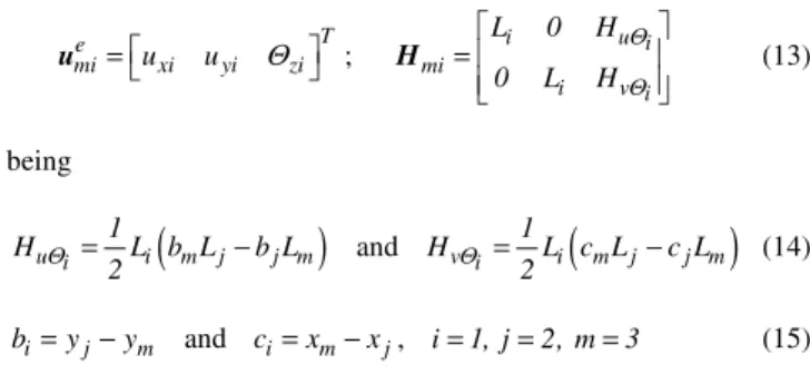
Results are presented in Fig 7. and Fig 8. and compared with those obtained by Yeom and Lee (1989) and a good agreement was obtained. These authors used 36 degenerated solid elements with nine nodes and five degrees of freedom per node. In this case the total number of nodes is 85. In the shell with hinged edges softening-stiffening responses with inflexion points are observed for
both stacking sequences, but this behavior is modified when hinged edges are substituted by clamped edges. It may be observed that results obtained in this paper are very similar to those of the reference with a mesh where a bi-quadratic degenerated quadrilateral element using Lagrangean polynomials as shape functions were substituted by two triangles with three nodes.
0,00 10,00 20,00 30,00 40,00 50,00 60,00 70,00 80,00 90,00 100,00
0,00 5,00 10,00 15,00 20,00 25,00 30,00 35,00
w (mm)
Load (
k
N
)
Yeom and Lee (clamped) Present work (clamped) Yeom and Lee (hinged) Present work (hinged)
Figure 7. Static response of a pinched cylindrical shell with a stacking sequence [0/90/0].
0,00 10,00 20,00 30,00 40,00 50,00 60,00 70,00 80,00 90,00 100,00
0,00 5,00 10,00 15,00 20,00 25,00 30,00 35,00
w (mm)
Lo
ad (k
N)
Yeom and Lee (clamped) Present work (clamped) Yeom and Lee (hinged) Present work (hinged)
Figure 8. Static response of a pinched cylindrical shell with a stacking sequence [45/-45].
Geometrically Nonlinear Dynamic Analysis of a Spherical Laminated Shell Under an External Uniform Pressure
An hinged spherical laminate shell is presented in Fig. 9, where
R(radius)=10.00 m, h(total thickness)=10.00x10⁻³m, b(length of the projected side)=1.00 m. The stacking sequence is an angle
ply 45 /−45 and the material properties are: E1=250.00 GPa, 2
E =10.00 GPa, G12=5.00 GPa, ν12=0.25 and ρ(specific
mass)=1.00 x10 kg / m8 3.Only one quarter of the shell was modeled using a mesh with 32 triangular elements (generated in
4 x4=16 rectangular regions) with 25 nodes, taking into account symmetry conditions. The following boundary conditions were prescribed: uy=Θx=Θz=0.00 on the line AB,
y x z
u =w=Θ =Θ =0.00 on the line BC, ux=w=Θy=Θz=0.00 on the line CD and ux=Θy=Θz=0.00 on the line AD. The
adopted time step and uniform pressure acting on the external
Figure 9. Hinged spherical shell subjected to a uniform external pressure.
The dynamic response at the central point A is shown in Fig. 10 and it is compared with the result presented by To and Wang (1998), and a good concordance is observed. In the present work the same response were obtained with the consistent and the lumped mass matrix.
To and Wang (1998) used the linear hybrid laminated composite triangular shell elements (HLCTS), with eighteen degrees of freedom and a first-order transverse shear deformation theory. These authors used a mesh with 36 triangular elements (generated dividing by four a region formed by 3x3=9 rectangles) with 25 nodes.
Teixeira (2001) used a modified consistent mass matrix taking into account only displacement degree of freedom, i. e. H in Eq.(78) was substituted by:
(
)
i i
i
L 0 0 0 0 0
0 L 0 0 0 0 i 1,2,3
0 0 L 0 0 0
= =
H . (79)
In both cases, in this specific example, results are close to those obtained by To and Wang (1998).
-0,10 0,00 0,10 0,20 0,30 0,40 0,50 0,60 0,70
0,00 0,25 0,50 0,75 1,00 1,25 1,50 1,75 2,00 2,25 Time (s)
w (m
m)
To and Wang Present work (consistent mass) Present work (modified mass)
Figure 10. Geometrically nonlinear dynamic response at the central point for the spherical shell.
Geometrically Nonlinear Dynamic Analysis of a Cylindrical Laminated Shell Subjected to an Uniform Internal Pressure
A cylindrical shell subjected to an uniform internal pressure is
R(radius)=2.54 m, a(arc length)=0.508 m, b(length)
0.508 m
= , h(total thickness)=1.27 x10⁻³m and ϕ(angle) 0.10 rad
= . Material properties are: E1=137.90 GPa,
2
E =9.86 GPa, G12=5.24 GPa, ν12=0.30 and
3
1562.20 kg / m
ρ = . Two stacking sequences were considered: (a)
a symmetric stacking sequence with eight layers 0 /−45 / 90 / 45 s
and (b) a cross ply 0 / 90. In both cases layers with the same thickness were adopted. It is considered that the shell boundary is clamped (ux=uy=w=Θx=Θy=Θz=0.00). The adopted time step and uniform internal pressure were, respectively,
2
t 5.00x10 ms
∆ = − and q=6895.00 Pa. A mesh with 128 elements (generated in 8 x8=64 rectangular regions) was used.
Figure 11. The cylindrical shell with uniform internal pressure.
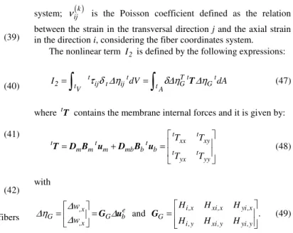
Results for the displacement component w (in the direction of the axis zg) are presented in Fig. 12 and Fig. 13 and comparison with those presented by To and Wang (1999) and Wu, Yang and Saigal (1987) are also shown. To and Wang (1999) used the HLCTS element while Wu, Yang and Saigal (1987) used a curved high-order quadrilateral shell element.
A good relatively agreement is observed, especially with respect to the response obtained by To and Wang (1999). These authors used a mesh with 36 triangular elements (originated dividing in four a region formed by 9 rectangles) with 25 nodes. Some differences may be observed with respect to the results (especially for amplitudes) presented by Wu, Yang and Saigal (1987). In this work a very refined mesh was used in order to confirm results obtained by To and Wang (1999) with respect to those presented by Wu, Yang and Saigal (1987).
q zg
yg
xg
A
xg
zg
yg
-1,00 -0,50 0,00 0,50 1,00 1,50 2,00 2,50 3,00
0,00 0,50 1,00 1,50 2,00 2,50 3,00 3,50 4,00 4,50 Time (ms)
w (m
m)
Wu, Yang and Saigal To and Wang Present Work
Figure 12. Nonlinear dynamic response for the vertical displacement at point A of the cylindrical shell with eight layers [0/-45/90/45]s.
0,00 0,20 0,40 0,60 0,80 1,00 1,20 1,40 1,60
0,00 0,50 1,00 1,50 2,00 2,50 3,00 3,50
Time (ms)
w (m
m)
Wu, Yang and Saigal To and Wang Present work
Figure 13. Nonlinear dynamic response for the vertical displacement at point A of the cylindrical shell with two layers [0/90].
Final Remarks
An efficient triangular finite element for the geometrically nonlinear static and dynamic analysis of laminate shells was presented in this work. The mass and the nonlinear stiffness matrix may be explicitly implemented. Results of all the examples show a very good agreement with those presented by others authors using different types of elements and formulations. In most of the examples the meshes employed in this work are less refined with respect to those used in the corresponding references.
By definition, stress components σzz, τxz and τyz are considered with a null value in the Classical Lamination Theory.
Actually these stress components are not null and they may assume important values in the layer interfaces causing delamination. Physically, one of the reasons of this failure mode is the fact that
zz
σ , τxz and τyz change significantly from one layer to the other
due to the abrupt differences of elastic properties. Thus, this theory is not suitable to study delamination.
In future works topics such as shells optimization analysis and shells with smart materials will be studied.
Acknowledgments
The authors wish to thank CNPq (Brazilian National Research Council) for its financial support.
References
Bathe, K-J., 1996, “Finite Element Procedures”, Ed. Prentice-Hall, New Jersey, United States of America, 1037 p.
Bathe, K-J. and Ho, L-W., 1981, “A Simple and Effective Element for Analysis of General Shell Structures”, Computers and Structures, Vol. 13, pp. 673-681.
Hibbit, Karlsson and Sorensen Inc., 1998, ABAQUS user´s Manual, version 5.8.
Jones, R. M., 1999, “Mechanics of Composite Materials” Ed. Taylor & Francis, Philadelphia, United States of America, 519 p.
Stegmann, J. and Lund, E., 2001, “Notes on Structural Analysis of Composite Shell Structures”, Aalborg University, Aalborg, 90 p.
Sze, K. Y., Liu, X. H. and Lo, S. H., 2004, “Popular Benchmark Problems for Geometric Nonlinear Analysis of Shells”, Finite Elements in Analysis and Design , Vol. 40, pp. 1551-1569.
Teixeira, P. R. F. 2001, “Numerical Simulation of the Interaction of Three Dimensional Compressible and Incompressible Flows with Elastic Structures using the Finite Element Method” (In Portuguese), Ph. D. Thesis, Federal University of Rio Grande do Sul, R.S., Brazil, 237 p.
To, C. W. S. and Wang, B., 1998, “Transient Responses of Geometrically Nonlinear Laminated Composite Shell Structures”, Finite Elements in Analysis and Design, Vol. 31, pp. 117-134.
To, C. W. S. and Wang, B., 1999, “Hybrid Strain Based Geometrically Nonlinear Laminated Composite Triangular Shell Finite Elements”, Finite Elements in Analysis and Design, Vol. 33, pp. 83-124.
Wu, C. Y., Yang, T. Y., Saigal, S., 1987, “Free and Forced Nonlinear Dynamics of Composite Shell Structures”, Journal of Composite Materials, Vol. 21, pp. 898-909.
Yang, Y-B. and Shieh, M-S., 1990, “Solution Method for Nonlinear Problems with Multiple Critical Points, AIAA Journal, Vol. 28, pp. 2110-2116.
Yeom, C. H., and Lee, S. W., 1989, “An Assumed Strain Finite Element Model for Large Deflection Composite Shells”, International Journal for Numerical Methods in Engineering, Vol. 28, pp. 1749-1768.
![Figure 7. Static response of a pinched cylindrical shell with a stacking sequence [ 0/90/0 ]](https://thumb-eu.123doks.com/thumbv2/123dok_br/18975585.455219/8.892.485.794.508.717/figure-static-response-pinched-cylindrical-shell-stacking-sequence.webp)

![Figure 12. Nonlinear dynamic response for the vertical displacement at point A of the cylindrical shell with eight layers [ 0/-45/90/45 ] s](https://thumb-eu.123doks.com/thumbv2/123dok_br/18975585.455219/10.892.95.419.138.355/figure-nonlinear-dynamic-response-vertical-displacement-cylindrical-layers.webp)
