New Analytical Approach to Nonlinear Behavior Study of
Asym-metrically LCBs on Nonlinear Elastic Foundation under Steady
Axial and Thermal Loading
Abstract
In this paper, nonlinear behavior analysis of an asymmetri-cally laminated composite beam (LCB) on nonlinear founda-tion under axial and in-plane thermal loading is considered. To solve the obtained governing equation, a novel method based on Laplace transform is used. The resulted approx-imate analytical solution allows us the parametric study of different parameters which influence the nonlinear behavior of the system. The numerical results illustrate that proposed technique yields a very rapid convergence of the solution as well as low computational effort. The accuracy of the pro-posed method is verified by those available in literatures. Keywords
Nonlinear analytical analysis; Laplace Transform; Asymmet-rically Laminated Composite Beam; Thermal loading; Non-linear elastic foundation
H. Rafieipour∗
, A. Lotfavar and M. H. Mansoori
Department of Mechanical and Aerospace En-gineering, Shiraz University of Technology, 71555-313 Shiraz, Iran
Received 19 Apr 2012; In revised form 09 May 2012
∗Author email: [email protected] [email protected]
1
1 INTRODUCTION
2
Beam is one of the important mechanical elements and has numerous applications in different
3
fields of engineering and industries such as civil, marine and aerospace structures or vehicles.
4
Among these, laminated composite beams with high stiffness and strength to weight ratio are
5
increasingly used in many engineering structures.
6
In most applications, they are subjected to non-linear vibrations which lead to material
7
fatigue and structural damage due to increment of the oscillation amplitude. Therefore, it is
8
necessary and very important to study dynamic nonlinear behavior and natural responses of
9
these structures at large amplitudes. Furthermore, it is desirable to provide an accurate
anal-10
ysis towards the understanding of the non-linear vibration characteristics of these structures.
11
Generally, it is often difficult to find an analytical solution for a given nonlinear problem
12
unless some simplifying assumptions are considered. Therefore, the application of different
13
numerical techniques seems to be obligatory. It should be noted that it is hard to have a
com-14
plete understanding of a nonlinear problem out of numerical results. Furthermore, numerical
15
difficulties appear if a nonlinear problem has singularities or multiple solutions.
However, closed form solutions are more interesting to research community even if they are
17
approximate solutions since they have various advantages such as ease of parametric studies and
18
considering of physics of the problem. Among approximate analytical solutions for nonlinear
19
problems, one may refer to the homotopy perturbation method (HPM) [8], the variational
iter-20
ation method (VIM) [9], the modified Lindstedt-Poincare method (MLPM)[11], the harmonic
21
balance method (HBM) [4], the energy balance method (EBM)[20], the parameter-expansion
22
method (PEM) [19] and He’s variational method (HVM) [12].
23
Most studies for nonlinear vibration and buckling analysis of beams are concerned with
24
isotropic and symmetrically LCBs, [1, 3, 6, 15, 16]. Due to the bending-stretching coupling
25
in asymmetrically laminated beams, their nonlinear vibrations analyses are significantly
dif-26
ferent from that of isotropic beams and symmetrically LCBs. A few studies can be found in
27
the literature for nonlinear analysis of asymmetrical LCBs [2, 7, 14]. For example, Patel et
28
al.[14] used a three-nodded shear flexible beam element in order to investigate nonlinear free
29
flexural vibrations and post-buckling of orthotropic laminated beams resting on a class of two
30
parameter elastic foundation. Gunda et al. [7] employed the Rayleigh-Ritz method to study
31
large amplitude vibration analysis of LCB with symmetric and asymmetric layup orientations.
32
Baghani et al. [2] employed the variational iteration method for large amplitude free vibrations
33
and post-buckling analysis of asymmetrically LCBs on nonlinear elastic foundation.
34
In this paper, geometrically nonlinear vibration and post-buckling analysis of
asymmet-35
rically LCB on nonlinear foundation under axial and in-plane thermal loading is considered.
36
First, Galerkin method is used and the governing nonlinear partial differential equation is
re-37
duced to a single nonlinear ordinary differential equation. Afterwards, a novel method based
38
on Laplace transform [13] that is called Laplace iteration method (LIM) is applied to obtain
39
analytical solution for the nonlinear governing equation. Finally, an approximate analytical
40
expression will be obtained which allows us to study effect of different parameters on
nonlin-41
ear behavior of the system. In this paper for the first time, the effect of thermal loading in
42
addition to the other effects is taking into account. The proposed technique yields very rapid
43
convergence of the solution as well as low computational effort.
44
2 SYSTEM DYNAMICS
45
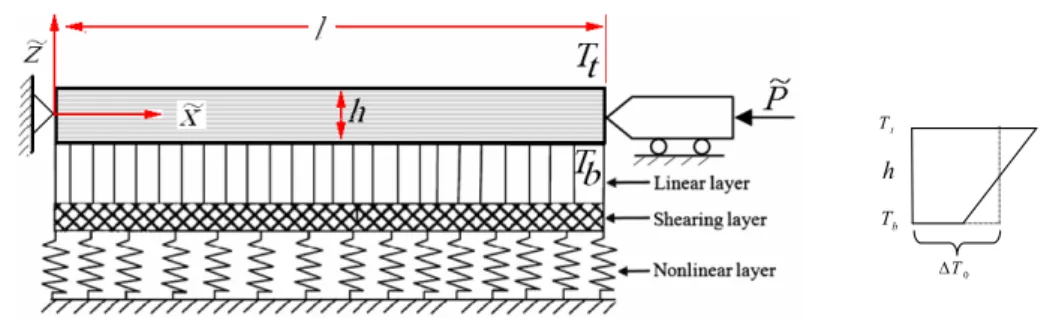
Consider a straight LCB of length l, width b, total thickness h and mass per unit length m
46
which rests on an elastic nonlinear foundation subjected to an axial force of magnitude ˜P and
47
a thermal load i.e. temperature varies linearly from Tb at bottom side to Tt at top side of the
48
beam as shown in Figure 1. A Cartesian coordinate is located while its origin is at left end
49
and its ˜x direction crosses through the neutral axis of the beam.
50
If ˜w and ˜uare the transverse and longitudinal displacements of the beam along the ˜zand
51
˜
x directions, respectively, ε0 shows the beam’s neutral axis strain, κ points up the flexural or
52
bending strain of the beam which is known as the curvature and εth represents the thermal
53
strain. Employing the Von Karman large deformation assumption, the strain–displacement
54
relation with considering thermal effect can be shown as [10]
Figure 1 Schematic of the straight LCB on a nonlinear foundation and subjected to an axial force and thermal loading
ε=εm+εth (1)
where
56
εm=ε0+zκ, ε˜ 0= ∂∂u˜˜x+12(
∂w˜
∂x˜) 2
, κ=−∂
2 ˜
w
∂˜x2, εth=αth∆T, ∆T =∆T0+z∆T˜ 1 (2) And ˜z measures the distance of beam’s material element from midline,αth is coefficient of
57
thermal expansion. Moreover, ∆T0 is temperature variation at midline of the beam and ∆T1
58
stands for temperature difference between top and bottom sides and they can be presented as:
59
∆T0= Tt +Tb
2 , ∆T1=
Tt−Tb
h (3)
The force and moment resultants per unit length based on the classical laminate beam
60
theory can be written as [10, 18]:
61
{ Nx˜ Mx˜ }
=[ A11 B11
B11 D11 ] { ε0
κ }−[
A11th B11th
B11th D11th ] {
∆T0 ∆T1 }
(4)
where its stiffness coefficients are given as follows [10, 18]:
62
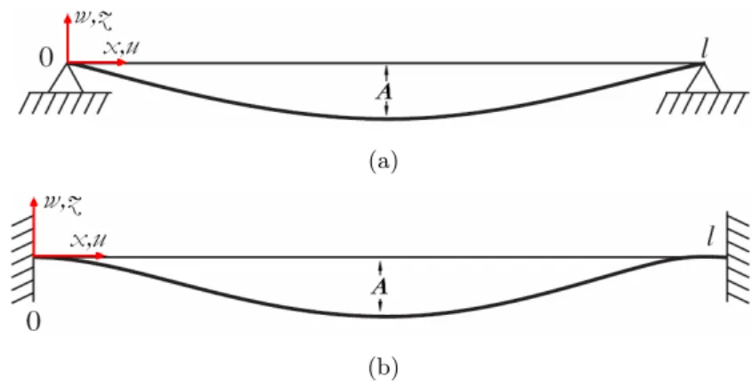
A11=
n
∑
k=1
¯
Q(11k)(hk−hk−1), A11th=
n
∑
k=1
¯
Q(11k)αth(k)(hk−hk−1)
B11= 12
n
∑
k=1
¯
Q(11k)(h2k−h2k−1), B11th= 1 2
n
∑
k=1
¯
Q(11k)α(thk)(h2k−h2k−1)
D11= 13
n
∑
k=1
¯
Q(11k)(h3k−h3k−1), D11th= 1 3
n
∑
k=1
¯
Q(11k)αth(k)(h3k−h3k−1)
(5)
Each layerkis referred to by the ˜z coordinates of its lower face (hk−1) and upper face (hk)
63
and ¯Q(11k) is the elements of the stiffness matrix in the ˜x direction,nis the number of laminas
64
and α(thk)is coefficient of thermal expansion of the kth layer.
65
Finally, using the Extended Hamilton’s principle [17, 18], the governing equation of
trans-66
verse vibration of an LCB including thermal effect and axial stretching on a nonlinear elastic
67
foundation can be obtained as
m∂ 2w˜
∂˜t2 +b(D11− B112 A11)
∂4w˜ ∂x˜4 +β
∂2w˜
∂x˜2 =Fw˜ (6) where
69
β=[P˜+b(A11th∆T0+B11th∆T1)−bA11 2l ∫
l
0(
∂w˜
∂x˜) 2
d˜x−bB11 2l (
∂w˜
∂x˜∣(l,˜t)−
∂w˜
∂x˜∣(0,˜t))]
Fw˜=−˜kLw˜−k˜N Lw˜3+k˜Sh∂
2 ˜
w ∂˜x2
(7)
˜
kL and ˜kN L are linear and nonlinear elastic foundation coefficients, ˜kSh is the shear stiffness
70
of the elastic foundation.
71
By defining non-dimensional variables
72
x= x˜
l, w=
˜
w
r, t=˜t
√
b
ml4γ, r=
√
I
A (8)
it can be written in a simple form as
73
∂2w ∂t2 +
∂4w
∂x4 +KLw+KN Lw 3
−KSh∂
2
w ∂x2
+[P+F0th+F1th−B∫01(
∂w ∂x)
2
dx−Λ(∂w∂x∣
(1,t)−
∂w ∂x∣(0,t))]
∂2
w ∂x2 =0
(9)
where r is the radius of gyration of the beam’s cross-section, and
74
KL=
˜
kLl 4
bγ KN L=
˜
kN Lr 2
l4
bγ KSh=
˜
kShl 2
bγ
P = P l˜
2
bγ F0th= l2
∆T0A11th
γ F1th= l2
∆T1B11th
γ
B= A11r 2
2γ Λ= B11r
γ γ =(D11− B2
11
A11)
(10)
To achieve the aims of the paper, the solution of Eq. (9) is assumed to be
75
w(x, t)=ϕ(x)η(t) (11)
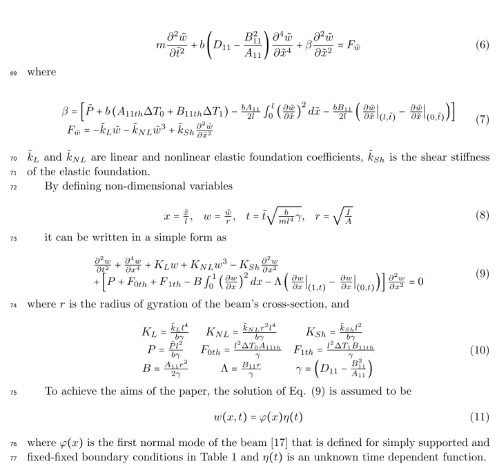
whereϕ(x)is the first normal mode of the beam [17] that is defined for simply supported and
76
fixed-fixed boundary conditions in Table 1 andη(t) is an unknown time dependent function.
77
Table 1 The first normal modes for beam with various boundary conditions
Boundary Condition ϕ(x)
Simply Supported ϕ(x)=sin(πx)
Fixed-Fixed ϕ(x)=(sinh(qx)−sin(qx))− sinh(q)−sin(q)
cosh(q)−cos(q)(cosh(qx)−cos(qx)), q=4.730041
Applying the Galerkin method [17], Eq. (9) yields
78
d2η(t)
dt2 +[α1+(P+F0th+F1th)αP +αL+αSh]η(t)+α2η 2(t)
(a)
(b)
Figure 2 The first normal functions of the beam with a) Simply supported, b) Fixed-Fixed boundary conditions
where
79
Now, it can be assumed that the beam is subjected to an initial displacement according
80
to its first modal shape and zero initial velocity. So, the initial conditions of Eq. (12) can be
81
presented as
82
α1= ∫
1 0ϕ
(iv)ϕdx
∫1 0ϕ
2dx , α2=−Λ(ϕ ′
(1)−ϕ′(0))αP, α3=−BαP ∫
1 0 ϕ
′2 dx
αP = ∫
1 0 ϕ
′′ϕdx ∫1
0ϕ
2dx , αSh =−KShαP, αL=KL, αN L=KN L
∫1 0ϕ
4
dx
∫1 0ϕ
2dx
(13)
η(0)=A, dη(0)
dt =0 (14)
where according to the Fig. 2, Adenotes the non-dimensional maximum amplitude of
oscilla-83
tion at the beam’s center.
84
Based on the Eq. (12) the nonlinear post-buckling load of the considered LCB can be
85
written as
86
PN B=−[α1+αP +αL+αSh]+α2A+(αN L+α3)A
2
αP −(
F0th+F1th) (15)
Neglecting the Ain Eq. (15), the linear buckling load will be derived as
87
PLB =−
α1+αP +αL+αSh
αP −(
F0th+F1th) (16)
The next step is to find the natural frequency of the system. Since the governing equation
88
Eq. (12) is nonlinear, the free vibration of the system has a nonlinear natural frequency
89
which is introduced by ωN L. Indeed, the nonlinear free vibration response of the system η(t)
90
and its nonlinear natural frequency ωN L depend on the system parameters, the boundary
91
condition and the initial conditions. Eq. (12) is strongly nonlinear and nobody can find an
92
exact analytical closed form solution for η(t) and ωN L. Although numerical methods can be
93
implemented to get over this problem but, they cannot offer any suitable way for parametric
study. Therefore, it will be valuable if a powerful analytical approximate method exists that
95
presents an accurate approximation ofη(t) andωN L while providing the ability to parametric
96
study of the problem.
97
3 DESCRIPTION OF THE PROPOSED METHOD
98
Using the Laplace Transformation method an analytical approximated technique is proposed
99
to present an accurate solution for nonlinear differential equations. To clarify the basic ideas
100
of proposed method consider the following second order differential equation,
101
¨
u(t)+N{u(t)}=0 (17)
with artificial zero initial conditions and N is the nonlinear operator. Adding and subtracting
102
the term ω2u(t), the Eq. (17) can be written in the form
103
¨
u(t)+ω2u(t)=L{u(t)}=f(u(t)) (18)
where Lis the linear operator and
104
f(u(t))=ω2u(t)−N{u(t)} (19)
Taking Laplace transform of both sides of the Eq. (18) in the usual way and using the
105
homogenous initial conditions gives
106
(s2+ω2)U(s)=I{f(u(t))} (20) wheres andI are the Laplace variable and operator, correspondingly. Therefore it is obvious 107
that
108
U(s)=I{f(u(t))} G(s) (21)
where
109
G(s)= 1
s2
+ω2 (22)
Now, implementing the Laplace inverse transform of Eq. (21) and using the Convolution
110
theorem offer
111
u(t)=
t
∫
0
f(u(τ) )g(t−τ)dτ (23)
where
112
g(t)=I−1{G(s)}= 1
Substituting Eq. (19) and (24) into (23) gives
113
u(t)=
t
∫
0
(ω2u(τ)−N{u(τ)})1
ωsin(ω(t−τ))dτ (25)
Now, the actual initial conditions must be imposed. Finally the following iteration
formu-114
lation can be used [5]
115
un+1=u0+ 1 ω
t
∫
0
(ω2un(τ)−N{un(τ)})sin(ω(t−τ))dτ (26)
Knowing the initial approximationu0, the next approximationsun, n>0 can be determined
116
from previous iterations. Consequently, the exact solution may be obtained by using:
117
u= lim
n→∞un (27)
In this method, the problems are initially approximated with possible unknowns and it can
118
be applied in non-linear problems without linearization or small parameters. The approximate
119
solutions obtained by the proposed method rapidly converge to the exact solution.
120
4 IMPLEMENTATION OF THE PROPOSED METHOD
121
Eq. (12) can be rewritten in the standard form Eq. (18)
122
d2η(t) dt2 +ω
2η(t)=f(η(t))
(28)
where
123
f(η(t))=ω2η(t)−N{η(t)}, λ1=α1+(P+F0th−F1th)αP +αL+αSh
N{η(t)}=λ1η(t)+λ2η2(t)+λ3η3(t), λ2=α2, λ3=(αN L+α3) (29)
Applying the proposed method, the following iterative formula is assembled
124
ηn+1(t)=η0(t)+ 1 ω
t
∫
0
f(ηn(τ))sin(ω(t−τ))dτ (30)
Eq. (28) will be homogeneous, if f(η(t)) is considered to be zero. So, its homogeneous
125
solution
126
η0(t)=Acos(ωt) (31)
is considered as the zero approximation for using in iterative Eq.(30).
127
Expanding f(η0(τ)), we have:
f(η0(τ))=(−λ1A+ω2A−3
4λ3A 3)
cos(ωt)−1 4λ3A
3
cos(3ωt)−1
2λ2A 2(
1+cos(2ωt)) (32)
Considering the relation:
129 1 ω t ∫ 0
(cos(mωτ))sin(ω(t−τ))dτ =⎧⎪⎪ ⎨⎪⎪ ⎩
cos(ωt)−cos(mωt)
ω2 (m2−1
) m≠1
tsin(ωt)
2ω m=1
(33)
To avoid secular terms in the next iterations, the coefficient of the cos(ωt) in f(η0(τ))
130
should be vanished. So the first approximation of the frequency is obtained as:
131
ω= √
λ1+3
4λ3A
2 (34)
Substituting Eq. (31) into (30) and neglecting the secular terms that are the coefficient of
132
cos(ωt) in forcing function f(η) give
133
η1(t)= 1
96ω2{(32λ2A 2
+96ω2A−3λ3A3)cos(ωt)+16λ2A2cos(2ωt)
+3λ3A3cos(3ωt)−48λ2A2} (35)
This is the first approximation ofη(t). Substituting Eq. (35) in Eq. (30) and implementing
134
the procedure for second time yields the second approximation ofη(t) as
135
η2(t)=
1 1981808640 1 A3 ⎛ ⎜ ⎝
I0+I1cos(ωt)+I2cos(2ωt)+I3cos(3ωt) +I4cos(4ωt)+I5cos(5ωt)+I6cos(6ωt) +I7cos(7ωt)+I8cos(8ωt)+I9cos(9ωt)
⎞ ⎟
⎠ (36)
where Iiare given in Appendix.
136
In this step, to avoid the secular terms the coefficient of cos(ωt) in forcing function must
137
be zero. So,
138
ω8+β6ω6+β4ω4+β2ω2+β0=0 (37)
where
139
β6=(−5
2 25λ3A
2
+13λ2A−λ1)
β4=(3
26λ 2
3A4−232λ2λ3A 3
+(215λ1λ3+ 5 2⋅3λ
2
2)A2−13λ1λ2A)
β2=(−3
2 212λ
3
3A6+215λ2λ 2
3A5+2⋅532λ 3
2A3−2795⋅3λ 2 2λ3A2)
β0=( 3
216λ 4
3A8−2312λ2λ 3 3A7+3
⋅5 29λ
2
2λ23A6−235⋅3)
(38)
Solution of Eq. (37) gives estimation ω for the actual natural frequency of the system.
5 NUMERICAL RESULTS
141
To illustrate the robustness of the proposed LIM method and to compare with other methods,
142
some cases are studied. First, an isotopic beam in two cases of simply supported and
fixed-143
fixed boundary conditions is taken. In these cases, the effects of thermal loading and elastic
144
foundation are ignored. The amounts of the nonlinear to the linear frequency ratioωN L/ωLare
145
derived for four non-dimensional amplitudes A. Table 2 shows the results of three references
146
as well as the numerical results that are computed by the fourth Runge-Kutta method in both
147
cases. The two last columns in each case show the results based on LIM and by one step and
148
two step iteration. As it is mentioned, the proposed method offers the results with excellent
149
accordance with the numerical results even by one step iteration.
150
Table 2 Comparison of nonlinear to linear frequency ratio,ωN L/ωL
Simply Supported Clamped–Clamped
Ref. Ref. Ref. Numerical Present Present Ref. Ref. Ref. Numerical Present Present
A [1] [16] [15] results[2] 1 step 2 step [1] [16] [15] results [2] 1 step 2 step
1 1.0891 1.0897 1.0897 1.0891 1.0892 1.0892 1.0221 1.0628 1.0572 1.0553 1.0566 1.0566 2 1.3177 1.3229 1.3228 1.3175 1.3179 1.3178 1.0856 1.2140 1.2125 1.2042 1.2058 1.2057 3 1.6256 1.6394 1.6393 1.6255 1.6263 1.6257 1.1831 1.3904 1.4344 1.4158 1.4179 1.4176
4 – – 1.9999 1.9758 1.9774 1.9761 1.3064 1.5635 1.6171 1.6658 1.6687 1.6679
In the second step, it is assumed that the composite beam is made by AS4/3501 Graphite–
151
Epoxy. Its mechanical properties [21] are E11 = 138GP a, E22 = 8.9GP a, υ12 = 0.3, α(1)th =
152
−0.5×10⁻⁶/○C and αth(2)=28.5×10
−6
/○
C. To study the effect of cross-ply lay-up configuration
153
on the nonlinear vibration of the considered LCB, three cases of configuration are used. Figure
154
3 illustrates this effect on the nonlinear to the linear frequency ratio ωN L/ωL and Figure 4
155
shows the influence on the ratio of the nonlinear post buckling load to buckling loadPN B/PLB
156
for both cases of boundary conditions, respectively. It can be seen that the nonlinear behavior
157
of the LCB with [0/90/90/0], [0/90/0/90] and [90/0/0/90] lay-up configuration increases from
158
lower values to higher values, respectively. So, the LCB behavioral response can be controlled
159
by its lay-up configuration, passively.
160
(a) (b)
(a) (b)
Figure 4 The effect of cross-ply lay-up configuration on the post bucking to the bucking load ratio Left) Simply supported, Right) Fixed-Fixed boundary conditions
(a) (b)
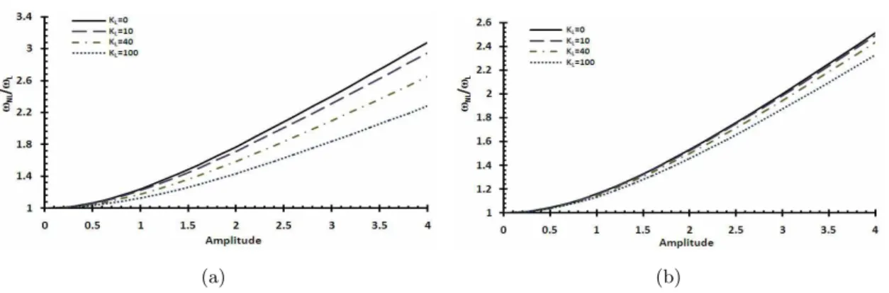
Figure 5 The effect of the linear stiffnessKLon the nonlinear to the linear frequency ratio
Left) Simply supported, Right) Fixed-Fixed boundary conditions
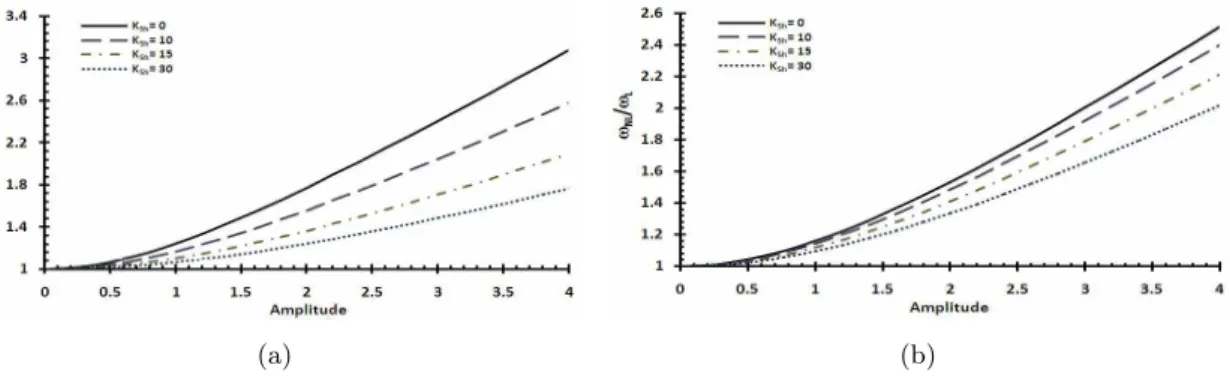
In the next step, the nonlinear behavior of the considered LCB due to elastic foundation is
161
investigated. As the [90/0/0/90] lay-up has the most critical nonlinear behavior, this
configu-162
ration is selected for the rest of the paper. Figure 5 to 7 demonstrate the effects of different
163
stiffness values of KL, KN L and KSh on ωN L/ωL ratio for both boundary conditions,
corre-164
spondingly. It can be seen that an increase in the linear and shearing layer stiffness of the
165
foundation leads to decrement of the nonlinear to linear frequency ratio and also an increase
166
in nonlinear stiffness augments this ratio. Also, the shearing layer stiffness has the strongest
167
effect.
168
Now, the axial loading is applied. Figure 8 shows the variation of the nonlinear to the
169
linear frequency ratio ωN L/ωL due to change in the axial loading P. It shows that axial
170
loading amplifies the nonlinear frequency ratio of the LCB.
171
Finally, the thermal loading is considered. As it is seen in Figure 9, thermal loading
172
increases the nonlinear to the linear frequency of the considered LCB. The results show that the
173
linear and nonlinear natural frequencies decrease by increasing the thermal loading however,
174
the decreasing rate of nonlinear frequency is less than linear natural frequency.
175
In the previous steps, the effect of each factor was studied, independently. So in the last
(a) (b)
Figure 6 The effect of the nonlinear stiffnessKN Lon the nonlinear to the linear frequency ratio
Left) Simply supported, Right) Fixed-Fixed boundary conditions
(a) (b)
Figure 7 The effect of the shear stiffnessKShon the nonlinear to the linear frequency ratio
Left) Simply supported, Right) Fixed-Fixed boundary conditions
(a) (b)
(a) (b)
Figure 9 The effect of the thermal loading on the nonlinear to the linear frequency ratio Left) Simply supported, Right) Fixed-Fixed boundary conditions For [0/90/0/90] lay-up configuration and L/h=50
walk, effects of all factors are implemented simultaneously. Table 3 and 4 show the results for
177
cases with simply supported and fixed-fixed boundary conditions, respectively.
178
Table 3 Comparison of nonlinear frequency(ωN L)and nonlinear to linear frequency ratio(ωN L/ωL)due to
change of different factors for S-S LCB, [0/90/0/90] lay-up configuration, A=2 and L/h=50
Nonlinear Frequency Nonlinear to linear Frequency
(Tt, Tb) P KL KN L KN L
0 50 0 50
Ksh Ksh Ksh Ksh
0 25 0 25 0 25 0 25
(0,0) 0 0 13.796 20.771 17.622 23.439 1.3978 1.1197 1.7855 1.2635
50 15.423 21.935 18.919 24.468 1.2703 1.1049 1.5583 1.2325
3 0 12.771 20.051 16.821 22.810 1.5510 1.1306 2.0428 1.2862
50 14.475 21.253 18.159 23.864 1.3336 1.1131 1.6730 1.2499
(50,50) 0 0 13.047 20.244 17.036 22.978 1.5001 1.1275 1.9587 1.2798
50 14.731 21.436 18.363 24.025 1.3142 1.1108 1.6382 1.2450
3 0 11.994 19.506 16.217 22.337 1.7676 1.1400 2.3900 1.3054
50 13.749 20.738 17.585 23.411 1.4030 1.1201 1.7944 1.2645
(150,50) 0 0 11.935 19.464 16.171 22.301 1.7915 1.1408 2.4273 1.3071
50 13.693 20.698 17.541 23.376 1.4095 1.1206 1.8055 1.2656
3 0 10.864 18.696 15.328 21.642 2.8264 1.1561 3.9877 1.3383
Table 4 Comparison of nonlinear frequency(ωN L)and nonlinear to linear frequency ratio(ωN L/ωL)due to change of different factors for F-F LCB, [0/90/0/90] lay-up configuration, A=2 and L/h=50
Nonlinear Frequency Nonlinear to linear Frequency
(Tt, Tb) P KL KN L KN L
0 50 0 50
Ksh Ksh Ksh Ksh
0 25 0 25 0 25 0 25
(0,0) 0 0 27.778 32.868 32.425 36.899 1.2416 1.1562 1.4493 1.2980
50 28.668 33.622 33.195 37.575 1.2218 1.1477 1.4147 1.2827
3 0 27.102 32.300 31.844 36.392 1.2586 1.1631 1.4788 1.3104
50 28.014 33.067 32.628 37.077 1.2361 1.1539 1.4396 1.2938
(50,50) 0 0 27.283 32.451 31.999 36.527 1.2539 1.1612 1.4706 1.3071
50 28.189 33.215 32.779 37.210 1.2321 1.1522 1.4327 1.2908
3 0 26.594 31.876 31.410 36.015 1.2729 1.1686 1.5034 1.3203
50 27.523 32.653 32.205 36.707 1.2478 1.1587 1.4601 1.3026
(150,50) 0 0 26.555 31.844 31.376 35.986 1.2740 1.1690 1.5053 1.3211
50 27.485 32.621 32.173 36.679 1.2487 1.1591 1.4617 1.3033
3 0 25.846 31.257 30.775 35.466 1.2963 1.1771 1.5435 1.3356
50 26.802 32.049 31.587 36.169 1.2669 1.1663 1.4931 1.3162
6 CONCLUSION
179
In this paper, the effects of different parameters such as vibration amplitude, nonlinear elastic
180
foundation, axial and thermal loading on the nonlinear behavior of the LCBs such as
natu-181
ral frequency and buckling load were investigated. For this purpose and to solve nonlinear
182
governing equation, a new approach based on the Laplace transform method which is called
183
LIM was implemented. This technique provides the ability for parametric study of the
consid-184
ered problem. Results revealed that the presented method offers accurate solution with low
185
computational effort.
186
Moreover, the presented expression is valid for a wide range of vibration amplitudes while
187
predictions of the other analytical techniques such as perturbation methods are valid for small
188
amplitudes. Comparison between the results of the present study and other methods available
189
in the literature shows the accuracy of the method. Results reveal that decreasing linear
190
and shear parameters and increasing nonlinear parameters of foundation lead to increasing
191
frequency and buckling load ratios. Furthermore, increasing axial force decreases absolute
192
values of both linear and nonlinear frequencies as well as natural frequency ratio.
193
Appendix: Ii coefficients in the second approximation of deflection.
194
I0=990904320A((Π1+21
16Π3−2Π4)A 2
+(− 1
32Π 2 3+(−
49 512Π5+
41
48Π4)Π3− 2 3Π
2 4)
A+( 13
4096Π 2 5+
31 72Π
2 4)Π3−
23 36Π
3 4)
I1=1981808640A4+(−54190080Π5−1052835840Π3−1101004800Π1−7741440Π2+1761607680Π4)A3
+(26512128Π23+(−595574784Π4+101007360Π5)Π3−7741440Π25+399114240Π24)A2+
I2=110100480A((Π1−3Π3+2Π4)A2+(− 1
64Π 2
3+(−2Π4− 51
1024Π5)Π3+2Π 2 4)
A+( 7 16Π 2 4+ 3 512Π 2 5)Π3−2
3Π 3 4)
I3=(7741440Π2+54190080Π5+61931520Π3)A3+( 8547840Π
2
3+(3870720Π5−45158400Π4)Π3
+5806080Π25+41287680Π24 ) A2
+((−181440Π25−16629760Π24)Π3−544320Π35+13762560Π34)A+15120Π45
I4=20643840A(A2Π3− 1
10Π3( 49
16Π5−6Π4+Π3)A+(− 2 45Π 2 4+ 3 320Π 2 5)Π3+
4 45Π
3 4)
I5=−483840A((Π2
3+(− 8 3Π5−
40
9 Π4)Π3−4Π 2
5)A+(− 32 27Π
2 4+
Π25 24)Π3+
Π35 8 )
I6=147456AΠ3((Π3+51
16Π5)A− 3 8Π 2 5+ 4 9Π 2 4) 195
I7=26880Π23A2+10080Π25(3Π5+Π3)A−945Π45 I8=3840Π52AΠ3 I9=189Π45
Where
196
Π1= λ1A 2
λ2
ω4 , Π2=
λ1A 3
λ3
ω4 , Π3=
λ2A 4
λ3
ω4 , Π4=
λ2A 2
ω2 , Π5=
λ3A 3
ω2
References
197
[1] L. Azrar, R. Benamar, and R.G. White. A semi-analytical approach to the nonlinear dynamic response problem of 198
s-s and c-c beams at large vibration amplitudes, part i: general theory and application to the single mode approach 199
to free and forced vibration analysis. J Sound Vib, 224:183–207, 1999. 200
[2] M. Baghani, R.A. Jafari Talookolaei, and H. Salarieh. Large amplitudes free vibrations and post-buckling analysis of 201
unsymmetrically laminated composite beams on nonlinear elastic foundation.Appl Math Model, 35:130–138, 2011. 202
[3] A. Barari. Non-linear vibration of euler-bernoulli beams.Latin American Journal of Solids and Structures, 8(2):139– 203
148, 2011. 204
[4] A. Bel´endez, A. Hernandez, T. Bel´endez, M.L. ´Alvarez, S. Gallego, M. Ortu no, and C. Neipp. Application of the 205
harmonic balance method to a nonlinear oscillator typified by a mass attached to a stretched wire. J Sound Vib, 206
302:1018–1029, 2007. 207
[5] E.Hesameddini and H. Latifizadeh. Reconstruction of variational iteration algorithms using the laplace transform. 208
Int J Nonlinear Sci Numer Simul, 10(10):1365–1370, 2009. 209
[6] S.A. Emam. A static and dynamic analysis of the post buckling of geometrically imperfect composite beams.Compos 210
Struct, 90:247–253, 2009. 211
[7] J.B. Gunda, R.K. Gupta, G.R. Janardhan, and G.V. Rao. Large amplitude vibration analysis of composite beams: 212
simple closed-form solutions. Compos Struct, 93:870–879, 2010. 213
[9] JH. He. Variational iteration method: some recent results and new interpretations. J Comput Appl Math, 207:3–17, 215
2007. 216
[10] L.P. Kollar and G.S. Springer.Mechanics of composite structures. Cambridge University Press, 2003. 217
[11] HM. Liu. Approximate period of nonlinear oscillators with discontinuities by modified lindstedt-poincare method. 218
Chaos Solitons Fractals, 23:577–579, 2005. 219
[12] J.F. Liu. He’s variational approach for nonlinear oscillators with high nonlinearity.Comput Math Appl, 58:2423–2426, 220
2009. 221
[13] A. Lotfavar, H. Rafieipour, and H. Latifizadeh. Application of the general variational iteration method to a nonlinear 222
system. InThe 2011 International Conference of Applied and Engineering Mathematics, ICAEM-127, volume 6, 223
pages 182–185, London, July 2011. 224
[14] B.P. Patel, M. Ganapathi, and M. Touratier. Nonlinear free flexural vibrations/post-buckling analysis of laminated 225
orthotropic beams/columns on a two parameter elastic foundation. Compos Struct, 46:189–196, 1999. 226
[15] T. Pirbodaghi, M.T. Ahmadian, and M. Fesanghary. On the homotopy analysis method for nonlinear vibration of 227
beams.Mech Res Commun, 36(2):143–148, 2009. 228
[16] M.I. Qaisi. Application of the harmonic balance principle to the nonlinear free vibration of beams. Appl Acoust, 229
40:141–151, 1993. 230
[17] S. S. Rao. Vibration of Continuous Systems. John Wiely & Sons, New Jersy, 2007. 231
[18] J. Reddy.Mechanics of Laminated Composite Plates Theory and Analysis. CRC, Boca Raton, 1997. 232
[19] D.H. Shou and JH. He. Application of parameter-expanding method to strongly nonlinear oscillators. Int J Nonlin 233
Sci Numer Simul, 8:121–124, 2007. 234
[20] D. Younesian, H. Askari, Z. Saadatnia, and M. KalamiYazdi. Frequency analysis of strongly nonlinear generalized 235
duffing oscillators using he’s frequency amplitude formulation and he’s energy balance method. Comput Math Appl, 236
59:3222–3228, 2010. 237
![Figure 9 The effect of the thermal loading on the nonlinear to the linear frequency ratio Left) Simply supported, Right) Fixed-Fixed boundary conditions For [0/90/0/90] lay-up configuration and L/h=50](https://thumb-eu.123doks.com/thumbv2/123dok_br/18884492.423507/12.892.183.757.103.322/figure-thermal-nonlinear-frequency-supported-boundary-conditions-configuration.webp)
![Table 4 Comparison of nonlinear frequency ( ω N L ) and nonlinear to linear frequency ratio ( ω N L / ω L ) due to change of different factors for F-F LCB, [0/90/0/90] lay-up configuration, A=2 and L/h=50](https://thumb-eu.123doks.com/thumbv2/123dok_br/18884492.423507/13.892.142.706.157.420/comparison-nonlinear-frequency-nonlinear-frequency-different-factors-configuration.webp)
