ISSN 0104-6632 Printed in Brazil
www.abeq.org.br/bjche
Vol. 31, No. 02, pp. 439 - 455, April - June, 2014 dx.doi.org/10.1590/0104-6632.20140312s00002359
Brazilian Journal
of Chemical
Engineering
A MIXED-INTEGER CONVEX FORMULATION
FOR PRODUCTION OPTIMIZATION OF
GAS-LIFTED OIL FIELDS WITH ROUTING AND
PRESSURE CONSTRAINTS
M. A. S. Aguiar
*, E. Camponogara and T. L. Silva
Department of Automation and Systems Engineering, Federal University of Santa Catarina C. P. 476, 88040-900 Florianópolis - SC, Brazil.
*E-mails: [email protected]; [email protected]; [email protected]
(Submitted: October 22, 2012 ; Revised: April 23, 2013 ; Accepted: April 28, 2013)
Abstract - Production optimization of gas-lifted oil fields under facility, routing, and pressure constraints has attracted the attention of researchers and practitioners for its scientific challenges and economic impact. The available methods fall into one of two categories: nonlinear or piecewise-linear approaches. The nonlinear methods optimize simulation models directly or use surrogates obtained by curve fitting. The piecewise-linear methods represent the nonlinear functions using a convex combination of sample points, thereby generating a Mixed-Integer Linear Programming (MILP) problem. The nonlinear methods rely on compact models, but can get stuck in local minima, whereas the piecewise-linear methods can reach globally optimal solutions, but their models tend to get very large. This work combines these methods, whereby piecewise-linear models are used to approximate production functions, which are then composed with convex-quadratic models that approximate pressure drops. The end result is a Mixed-Integer Convex Programming (MICP) problem which is more compact than the MILP model and for which globally optimal solutions can be reached.
Keywords:MINLP; MILP; Mixed-Integer Convex Programming; Oil Production Optimization.
INTRODUCTION
With the increasing demand for fossil energy, the oil industry has looked for new technologies in hardware and software to enable production optimi-zation of oil fields. These are evolving technologies often referred to as smart fields (Williams and Webb, 2007; Moisés et al., 2008). However, before this con-cept is transferred to the oil fields, significant chal-lenges in science and technology should be over-come. To this end, this paper addresses the problem of optimizing production of oil fields operated with artificial lifting and subject to facility, routing, and pressure constraints.
Large oil fields have several production wells spread over a wide area. The production of clusters of
The production optimization problem consists of a Mixed-Integer Nonlinear Programming (MINLP) problem for which the direct application of standard algorithms may not be possible or effective. This problem is only known conceptually because the well-production functions and pressure-drop rela-tions are not explicitly available. The proposed solu-tion approach uses two-dimensional piecewise-linear models for the well-production functions that depend on the lift-gas rate and manifold pressure, while continuous convex functions are used to approximate the three-dimensional pressure-drop functions. The continuous convex approximation has the advantage of being quite compact when compared to three-di-mensional piecewise-linear models. In the end, the production optimization problem is approximated as a Mixed-Integer Convex Programming (MICP) prob-lem which can be tackled with off-the-shelf solvers. Computational experiments are performed to compare the MICP formulation and a Mixed-Integer Linear Programming (MILP) formulation obtained by piecewise-linearizing the pressure drops, which is more precise but demands a large number of sample points. The MICP formulation is further compared with an MINLP formulation obtained from MICP by imposing a precise pressure-balance in the flow lines. The computational experiments assess the trade-off between solution speed and the degree of approximation across formulations. A simulation analysis is carried out to compare the mean errors of the field variables predicted with the formula-tions, against the variables obtained with a multi-phase-flow simulator. Because the true MINLP prob-lem is only known conceptually, this analysis serves the purpose of comparing the effectiveness of the ap-proximations and identifying how complex the under-lying models need to be to represent the production process satisfactorily.
In what follows, the production optimization problem is first formalized in mathematical notation. Background is presented on multidimensional piece-wise-linear (PWL) and quadratic programming (QP) models, which are then used in the problem formula-tion. Computational and simulation results are reported and discussed. Finally, the paper ends by offering some concluding remarks and suggesting directions for future research.
PROBLEM DEFINITION
In several offshore fields, oil production relies on artificial-lifting methods to compensate for low res-ervoir pressure and high depth resres-ervoirs, notably the
ones located off the coast under the sea bed. Among the artificial-lifting methods, gas-lift is a widely ap-plied technique for its desirable features that include relatively low installation and maintenance costs, robustness for using few mechanical components, and efficiency. It works by injecting high pressure gas at the bottom of the production tubing to induce a pressure gradient from the reservoir all the way up to the surface facilities.
When the operating conditions on the surface are kept constant or change slowly, the modeling of well production can be carried out using Well Performance Curves (WPCs), which relate the production of oil, gas, and water to the lift-gas injection rate. Several works in the technical literature (Buitrago et al., 1996; Alarcón et al., 2002; Camponogara and Nakashima, 2006; Camponogara and de Conto, 2009; Misener et al., 2009; Codas and Camponogara, 2012) have ad-dressed the problem of optimizing production for pre-determined surface conditions.
However, when surface conditions change fre-quently due to routing operations, failure of equip-ment, and shutting operations of wells, the standard WPC modeling needs to be extended to consider the pressure at the manifolds which concentrate produc-tion from the wells (Kosmidis et al., 2004). Some works from the literature take into account pressure balance constraints (Litvak et al., 1997; Kosmidis et al., 2004; Bieker, 2007; Gunnerud and Foss, 2010; Silva et al., 2012; Codas et al., 2012; Silva and Camponogara, 2014), with some approaches using nonlinear functions and others relying on piecewise-linear models to approximate pressure drops through pipelines.
A Mixed-Integer Convex Formulation for Production Optimization of Gas-Lifted Oil Fields with Routing and Pressure Constraints 441 concave for a varying lift-gas injection rate, provided
that the well-head pressure is kept at the nominal value and the well does not have a kick-off rate.
The definition of the Production Optimization Problem (POP) is based on the following parameters:
= { , , }¼
N
is the set of oil wells, N being their number, and mÍ is the subset of wells that have a flow line connected to manifold m; ={ , , }¼ M is the set of manifolds, M being the number of manifolds, and nÍ is the subset of manifolds that can receive production from well
n, which is then transferred to a single separator;
={o,g,w} has the multiphase flows: oil o ,
gas g and water w ;
max
i
q is the lift-gas limit supplied by the com-pressors;
qin,min and qin,maxare operational limits for lift-gas injection into well n;
pm,S is the nominal pressure of the separator that receives production from manifold m;
qn,L and qn,Uare the lower and upper bound on the flow rate of well n;
variables:
qin is the lift-gas rate allocated to well n;
n
y is 1 when well n is producing, and 0 other-wise;
,
n m
z takes value 1 if the production from well n
is directed to manifold m, and 0 otherwise;
n m,
h
q is the flow of phase hÎ sent from well
n to manifold m and qn m, = qh:hÎ is a vector with all phase flows. The gas flow rate received by the production manifold is the sum of the lift-gas injected into well n (Inj) and the gas from the
reservoir (R): qgn m, =qg,Rn m, +qg,Injn m, ;
,
Î
=
å
q q
m
m n m
n is the total flow received from the wells connected to manifold m for all phases;
pm is the pressure of manifold m; and functions:
g is the profit function of the oil and gas production that accumulates in a manifold;
c is the cost function for lift-gas injection into a well;
qn m, pm,qin is the production function of well n
if connected to manifold m as a function of the
mani-fold pressure pm and the lift-gas injection rate qin;
Δpm qm is the pressure drop in the flow line connecting manifold m to its dedicated separator as a function of the multiphase flow qm.
Then the production optimization problem con-sidering a group of gas-lifted wells, routing decisions about well-manifold connections, and lift-gas, sepa-rator flow handling, and pressure constraints can be conceptually formalized as an MINLP problem:
POP: m n
m n
f g c qi
max
Î Î
=
å
q -å
(1a)
st.: i imax
Î
£
å
n n
q q (1b)
,min ,max
in n£ in£ in n," Î
q y q q y n (1c)
, ,
Î
= " Î
å
n
n m n m
z y n (1d)
n m n m m n
n m n
p q z
( n m
, ,
i ,
, , ,
= " Î " Î
q q (1e)
,L , ,U ,
Î
£
å
£ " Îq q q
n
n n m n
n n
m
y y n (1f)
, ,
Î
=
å
" Îq q
m
m n m
n
m (1g)
,min£ £ , max," Î
qm qm qm
m (1h)
m m m m
p =p ,S+Δp q ," Îm (1i)
n
y Î{ , }," În (1j)
n m n
z , Î{ , }," În ," Îm (1k)
The restriction given by Eq. (1b) says that there is a limited amount of lift-gas. Eq. (1c) says that the gas injection in an individual well is limited by an upper and lower bound if the well is producing when
= n
y , otherwise this injection is zero when =
n
y . Eq. (1d) ensures that each well must be
con-nected to a single manifold when the well is
produc-ing. Eq. (1e) defines the multiphase flow qn m, from well n to manifold m as a function of the manifold
pressure pm and the lift-gas injection qin. Eq. (1f) restricts the multiphase flow of a well n to be within lower and upper bounds when the well is operating (yn= ). Eq. (1g) ascertains that the inflow into a manifold m is precisely the sum of the multiphase flows from the connected wells. Eq. (1h) establishes processing capacity for the separators. Eq. (1i) ensures the pressure balance in the flow lines, namely that the difference between the manifold pressure and its separator is precisely the pressure drop through the flow line.
The MINLP problem given in Eq. (1) is a concep-tual definition of the production optimization problem,
since the well-production function qn m, pm,qin and the pressure drop Δpm qm are not known explicitly. Correlations can be found in the literature and are often available in simulation software for approxi-mating pressure relations in oil production systems (Beggs and Brill, 1973; Litvak and Darlow, 1995). Although one could conceivably model qn m, and Δpm with these correlations, the resulting MINLP formu-lation would be highly nonlinear and complex, ren-dering a global optimization problem, which is a chal-lenge for existing algorithms and software. This work is half-way between the approaches that use piecewise-linear models and those that rely on non-linear correlations. Instead, the well-production tions will be approximated with piecewise-linear func-tions and the pressure drops with convex funcfunc-tions.
PIECEWISE-LINEAR AND QUADRATIC CONVEX APPROXIMATIONS
Two favorite strategies for solving the production optimization problem are nonlinear programming methods and MILP strategies which rely on models obtained by piecewise linearizing the nonlinear functions. While the former method is prone to get stuck in local minima, the latter method can lead to very large MILP problems.
This work suggests a hybrid approach that ap-proximates the pressure drop functions with convex functions and the well-production functions with piecewise-linear models. Such an approach renders the approximation problem an MICP program which is far more compact than the MILP approximation and which can be solved efficiently up to optimality.
Convex Combination Model
Among the MILP models for piecewise lineariza-tion available in the literature (Vielma et al., 2010), this work uses the Aggregated Convex Combination (CC) model to approximate the well-production func-tion qn m, . Let f : be a continuous function defined over a compact domain Íd. According to Vielma et al. (2010), f is piecewise-linear if and only if there exists a family of polytopes , such that
Î =
P P , { }
Î Ì
mP P d, {c }P PÎ and further:
P
f x =m xT +cP, xÎ " ÎP P, (2a)
Let V P be the set of vertices of polytope P and
PÎ V P
=
be the set of all vertices. The CC model assigns weighting variables to each vertex
Î
v . Thus a graph point is represented by
f λ f
, ,
Î
=
å
vv
x x v v
where { }λv vÎ Ì+
and λ
Î
=
å
vv
. The CC model is given by:
, Î
=
å
vv
v x
λ λ f f
Î
=
å
vv
v x
(3a)
, ,
³ " Î
v v
λ Î
=
å
vv
λ (3b)
( )
, ,
Î
£
å
" Î vv v
P P
λ y
Î
=
å
P P
y (3c)
P
y Î{ , }," ÎP (3d)
where v : {= PÎ:vÎV P } is the set of poly-topes that contain vertex v.
The constraints (3a) represent a graph point f
,
A Mixed-Integer Convex Formulation for Production Optimization of Gas-Lifted Oil Fields with Routing and Pressure Constraints 443 ensure that the λ weights define a convex
combina-tion of the vertices and funccombina-tion values. Equacombina-tions (3c) limit convex combinations to a single polytope, and further guarantee that only the weighting vari-ables associated with vertices of the active polytope can be non-zero.
Convex Quadratic Model
A convex quadratic approximation of a nonlinear function f :n consists of
f x » x x b xTQ + T +c (4a)
where Q is a positive definite matrix denoted by
Q , b is a vector, and c is a constant. Such quadratic functions will be used later to approximate pressure-drop relations, since their behavior is dominated by the effects of friction, which depends on the square of the flow speed.
PROBLEM APPROXIMATION
This section begins by presenting the piecewise-linear modeling of well production, followed by the convex quadratic approximation of pressure drop and the synthesis of such models. These models are then combined to obtain the MICP formulation for oil production optimization.
Piecewise-Linear Approximation of Well Production Functions
The multiphase flow function qn m, pm,qin depends on the pressure of the manifold m to which this well is connected,pm, and the lift-gas injection rate qin. Using the CC model, the piecewise-linear approximation of well production is formulated as follows:
For allnÎ :
i r
, ,
i r
,
i , i
Î Î Î
=
å å å
n n m n m
n n m
q p
m q p
q λ q (5a)
n m n m
n m m
n q p
q p
λ p p m i r , , i r , r , , Î Î
£ " Î
å å
(5b)
i r , , i r , ,max r , , , Î Î £ + -" Î
å å
n m n mm n m m
n m q p
q p
n
p λ p p z
m (5c) i r , , i r , , , i r , , , Î Î = " Î
å å
q q
n m n m
n m n m n m
q p
q p
n
λ q p
m (5d) i q i r , , , r , ³ " Î, ," Î , " Î
n m n m n m
n q p
λ m p (5e)
i r , , i r , , , , Î Î
= " Î
å å
n m n m n m
n m n
q p
q p
λ z m (5f)
i r , i r , , , i , , , r , , , Î
£ " Î " Î
" Î
å
n m
n m n m n m
P n
q p
P q p
n m
λ δ m q
p (5g) , , , , Î
= " Î
å
n m n m
P n m n
P
δ z m
(5h)
n m n m
P n
δ , Î{ , }," Îm ," ÎP , (5i)
having the following extra parameters:
n m, and n m, are the sets of breakpoints for the lift-gas rate and manifold pressure when well n is connected to manifold m, respectively;
n m, is the set of polytopes with vertices in
, ,
n m´ n m
;
n m, q pi, r ={PÎn m, : q pi, r ÎV P } has the polytopes that contain vertex q pi, r ;
pm,max is the maximum manifold pressure; and extra variables:
i r , , n m q p
λ is the weighting variable of a breakpoint
pair in n m, ´n m, ;
dn mP, is a binary variable for each polytope
, n m
of the convex combination defining the gas injection into well n and manifold pressure pm;
q ,n m is the piecewise-linear approximation of ,
n m q .
Notice that the injection bound (1c) and the well-production restriction (1f) are implicitly imposed by the piecewise-linear approximation, i.e., the infeasi-ble points do not belong to the domain of the PWL approximation function.
Convex Quadratic Approximation of Pressure Drop Functions
The approximation of the pressure drop in the flow-line from a manifold m to its separator is approxi-mated with a convex quadratic function. Thus, for all
mÎ:
,
m
m n m
nÎ
=
å
q q
(6a)
Δpm= qm TQmqm+b qTm m+cm (6b)
,S Δ m
m m
p =p + p (6c)
where Qm . Being an equality, Eq. (6c) induces a nonconvex and discontinuous set of candidate solu-tions, which results in a nonconvex approximation of the production optimization problem. However, this equality may be approximated by two convex ine-qualities:
,S
ue
Δpm £pm-pm (7a)
,S
oe
Δpm³pm-pm (7b)
with Δpuem being a convex underestimation and Δpoem being a concave overestimation of the pressure drop
Δpm. Replacing (6b)-(6c) with (7) would lead to a relaxation of the true MINLP. Notice that a problem
: R max{ R : }
R z = f x x X RÎ is a relaxation for
a problem P z: P=max{f x x X PP : Î } if X R ÊX P and f xR ³f xP for all x X PÎ . Provided that the piecewise-linear models of the production functions are precise, the optimal solution
to the MICP arising from this replacement would induce an upper bound on the objective. The ability to produce relaxations based on under and overesti-mation within a reduced domain of the decision space, possibly using convex and concave functions as given in (7), would allow the application of a spatial branch and bound strategy.
The physical behavior in the oil production system is such that, for a given pressure difference
,S
m m
p -p the flow qm will be as large as possible and, thereby, so will be the pressure drop Δpm qm . This means that constraint (7b) may not be bounding and the approximation of (6b)-(6c) can be carried out only with (7a). Since the effectiveness of this ap-proximation should be assessed by simulation of the oil field, we will consider a general single-sided approximation of the form:
,S
Δpm£pm-pm (8a)
where Dpm is a convex function that meets one of the following cases:
1) Underestimation: if Δpm qm £Δpm qm for all qm, then (6b)-(6c) can be approximated by:
, , m
m S m m m S m
p +Dp -p £ p +Dp -p £ (9a) meaning that the resulting MICP formulation will be a relaxation for the true problem, provided that the piecewise-linear functions for well production can be regarded as precise models and the objective function is not modified.
2) Overestimation: if Dpm qm ³Dpm qm for all qm, then (6b)-(6c) is approximated by:
,
,
m
m S m
m S m m
p p p
p p p
D - £
-+D £
+
(10a)
3) Estimation: when Δpm qm neither under-estimates, nor overestimates the true pressure drop, an approximation for (6b)-(6c) is given by:
, m
m S m m
p +Dp -p -e £ (11a)
m
A Mixed-Integer Convex Formulation for Production Optimization of Gas-Lifted Oil Fields with Routing and Pressure Constraints 445 The excess εm may be necessary to ensure
feasi-bility of the MICP formulation when Δpm is an over-estimation. Notice that the excess εm can be nullified
when Δpm£pm-pm,S, otherwise εm should be driven to zero. One possibility is to introduce in the objective a penalty factor on the excess, such as
m e
-m with m > . As m tends to zero the penalty increases, drawing εm towards the origin unless a feasible solution with εm = does not exist. The strategy of introducing an excess variable is also viable for the case of overestimation.
To obtain the MICP formulation, the choice among the cases above should be based on an analysis of the approximation quality and validated through simulation.
Curve Fitting for Quadratic Approximation of Pressure Drop
Two relevant issues are how convex-quadratic approximations for the pressure drop are computed and whether or not such approximations are satisfac-tory. To resolve these issues, we suggest solving a Semi-Definite Program (SDP) minimizing the error with respect to a set of pressure-drop points obtained from field data or multiphase-flow simulators. The synthesis of the convex-quadratic approximation for
Δpm consists in solving the following problem:
CF :
, ,
,
Δ Δ
Δ , ,
m k m k
m k k
m m m
p p
min
p
Q c Î
-å
b
(12a)
s.t.: Δ , , , ,
,
m k m k T m k m k
m Tm
m
p Q
c k
= +
+ " Î
q q b q
(12b)
m mT
Q =Q (12c)
, ,
m m m
Q Î ´ b δ c Î (12d)
where = ¼{ , , }K is the set of indexes of the pressure-drop sample points qm, , Δpm, , , ¼ qm K, ,
,
Δpm K . Notice that CF can be easily recast as an SDP by linearizing the objective function with the
introduction of slack variables and linear inequali-ties, namely by expressing the l -norm of the vector of approximation errors as a system of linear ine-qualities. Reformulations of CF in SDP are briefly discussed in the Appendix.
The choice of convex approximation, the l -norm, and the relative error in the objective function was not arbitrary but rather the result of experimental analyses. For instance, the pressure-drop approxima-tions obtained by minimizing concave funcapproxima-tions were consistently worse than the minimization of convex functions. The experiments also revealed that the error should be normalized because pressure drops can vary drastically from low to very high values.
The analyses leading to these findings will be presented later in the paper.
Piecewise-Linear Convex-Quadratic Approximation
By piecewise-linearizing the well-production function qn m, using the CC model and representing
the pressure drop Δpm with a convex-quadratic function, the oil production optimization problem is approximated by an MICP problem:
i
: max
m n
m n
m
m
POP f g c q
Î Î
Î
m =
-- e
m
å
å
å
q
(13a)
s.t.: in imax
n
q q
Î
£
å
(13b)
For all nÎ :
i r
, ,
i r
,
i q ,p i
q p
q
n m n m n
n n m
m q
Î Î Î
=
å å å
λ (13c)
i r
, ,
i r
, r q ,p
q p
p ,
n m n m
n m m
n
p m
Î Î
£ " Î
å å
λ (13d)
i r
, ,
i r
, ,max r , q ,p
q p
p ,
n m n m
m n m m
n m
n
p p z
m
Î Î
£ +
-" Î
å å
λ
i r , , i r , , , i r q ,p q p
q ,p ,
n m n m
n m n m n m
n m Î Î = " Î
å å
q q
λ (13f) i r , , , i r q ,pnm ³ " Î, m n, q" În m, p" Înm
λ (13g)
i r , , i r , , q ,p q p ,
n m n m
n m
n m n
z m
Î Î
= " Î
å å
λ (13h)
r i i , , ,
q ,p i ,
r ,p , , , , n m r n m
n n m
P P q n m n m m q p Î
£ d " Î " Î " Î
å
λ (13i) , , , , n m n mP n m n P
z m
Î
d = " Î
å
(13j)
,
n
n m n m z y Î =
å
(13k)For all mÎ:
,
m
m n m
nÎ
=
å
q q
(13l)
,min , max
m £ m£ m
q q q (13m)
,S Δ m
m m m
p + p -p -e £ (13n)
m
e ³ (13o)
, { , }, , ,
n m n m
P m n P
d Î " Î " Î (13p)
{ , } ,
n
y Î " În (13q)
, { , } , ,
n m n
z Î " În " Îm (13r)
where Δpm:= qm TQmqm+b qTm m+cm
The approximation error for the well-production
functions is controlled by the number and location of breakpoints. On the other hand, the pressure-drop error depends on the quadratic models obtained by SDP optimization, but also on the penalty factor m. Let w m be a vector with the solution to POP m . Our solution strategy consists in solving a problem sequence {POP mk } with decreasing mk until
approximation errors εm are sufficiently small. At iterationk , problem POP mk is solved starting
from w mk- which is feasible for POP mk .
Notice that the POP mk formulation
encom-passes the three cases considered for Δpm. If Δpm is an underestimation, then εm will be driven to zero by the suggested iterative strategy and POP m will induce an upper bound when εm = for all m. In this case, the excess variables and the penalty factors can be removed altogether, allowing POP m to be solved only once since it will be unaffected by the
choice of m. On the other hand, when Δpm over-estimates the true pressure drop, POP m will be a handy approach to find a nearly optimal solution when the problem becomes infeasible without the excess variables.
Fully Piecewise-Linear Approximation
The MILP approximation for the oil production optimization problem is obtained from POP m by eliminating the excess variables εm, along with the penalty factor in the objective function, and re-placing (13n) with a three-dimensional piecewise-linear formulation using the CC model:
o g w o g w
o g w, , , , , ,
Ω
m
m m m
k k k k k k
k k k Î
=
å
q q
(14a)
o g w o g w, , , ,
o g w
.
Δ Ω
Δ , ,
m
m m
k k k k k k
m
p
p k k k Î
=
å
(14b)
,S Δ m
m m
p =p + p (14c)
o g, , w o g w
A Mixed-Integer Convex Formulation for Production Optimization of Gas-Lifted Oil Fields with Routing and Pressure Constraints 447
o g w
o g w , ,
, ,
o g w
Ω ,
, ,
m
m m
P k k k
P k k k
m y
k k k Î
£
" Î
å
(14e)
m
m m
P P
y y
Î
=
å
(14f)
o g w o g w, , , ,
Ω
m
m m
k k k k k k
y Î
=
å
(14g)
,
m
m
n m n
y z
Î
£
å
(14h)
{ , } m
y Î (14i)
{ , } ,
m m
P
y Î " ÎP (14j)
with the parameters:
o g w
, ,
m k k k
q is the fluid flow of oil ko , gas
g
k , and water kw of the vertex k k ko, ,g w in the domain ofΔpm;
m is the set of polytopes whose union defines the domain of the pressure-drop function;
m k k ko, g, w Ím is the set of polytopes that contain vertex k k ko, ,o w ;
m is the se of all vertices appearing in the
set of polytopes m; and the additional variables:
yPm is a binary variable associated to polytope m
PÎ which assumes the value 1 when the convex combination is confined toP ;
o g w
, ,
Ωmk k k is a variable with the weight
associ-ated to vertex k k ko, g, w Î ;
ym is an auxiliary binary variable which takes on the value 1 when manifold m receives production.
As before, the bound constraint (13m) is implic-itly imposed by the domain of the PWL approxima-tion of the pressure-drop relaapproxima-tion.
COMPUTATIONAL ANALYSIS
This section evaluates the MICP formulation com-putationally. First, a synthetic oil field is instantiated
in a commercial multiphase-flow simulator honoring the characteristics of real-world oil fields. Break-points for well-production functions and pressure drops in flow lines are obtained by sampling the simulator, which are used to yield piecewise-linear models for qn m, and quadratic approximations for Δpm. Finally, the performance and solution quality of the MICP formulation is compared with the MILP formulation and an MINLP formulation obtained from MICP.
Oil Field Scenario
Inspired in a scenario from (Kosmidis et al., 2004), a synthetic oil field was put together for the purpose of computational and simulation analysis (Silva et al., 2012). This field consists of two separators with a limited separation capacity and an operational pres-sure of 300 psia pm,S .
Figure 1 illustrates the structure of the gathering system of the synthetic oil field. Separator 1 is con-nected to an adjoint manifold by a flow line of 100 m, whereas separator 2 is connected to another manifold by a flow line of 50 m. All of the 16 gas-lifted oil wells can be routed to one of the manifolds; how-ever, wells 1 to 8 are closer to manifold 1, while wells 9 to 16 are closer to manifold 2. The wells are limited in the amount of fluids they can handle and lift-gas injection rates should be within bounds when the wells are producing.
The oil field was modeled with the Pipesim simulator, which allowed us to obtain breakpoints for piecewise-linearization of the well-production func-tions and pressure-drop points for the synthesis of quadratic approximations.
Figure 1: Gas-lift production network.
Approximation Analysis of Pressure Drop
the visual analysis was not possible, the concave- and convex-quadratic fittings of the sample data (pressure drop) were analyzed. The different strate-gies considered for pressure-drop approximation with quadratic functions are shown in Table 1.
Table 1: Pressure drop approximation strategies. Function type Concave
Convex
Norm
l -norm l -norm l¥-norm
Error type Absolute Error (min
a
e ) Relative Error (mine%)
To find the approximations according to the strategies of Table 1, the corresponding variations of the curve fitting problem CF , given in Eq. (12), were implemented in YALMIP (Löfberg, 2004) and solved with the SDP solver SeDuMi version 1.3 (Peaucelle et al., 2002). The curve fitting problems were solved in a workstation running Ubuntu Linux with 64 bits. Eq. (12c) was replaced with
m mT
Q =Q for the concave approximation, while Eq. (12a) was modified depending on the error type and norm. In all, 729 breakpoints consisting of the combination of 9 gas-flow rates (in the range from 137,777 to 1,240,000 m3/d), 9 oil-flow rates (from 400 to 3,600 m3/d), and 9 water-flow rates (from 92.2 to 830 m3/d) were sampled from Pipesim.
Intending to compare the curve fitting strategies, we established four quantitative indexes consisting of the maximum and mean values for the absolute
(
e
a) and relative error (e
%) induced by the resulting quadratic formulations. Table 2 shows these quanti-tative indexes with absolute errors given in psia and relative errors given in percentage.The experiments are characterized by a tuple
, ,
m m m where m Î{convex, concave} indicates the curvature, m Î{ , , } l l l¥ indicates the error vector norm, and m Î{min , min }ea e% indicates minimiza-tion of absolute or relative error.
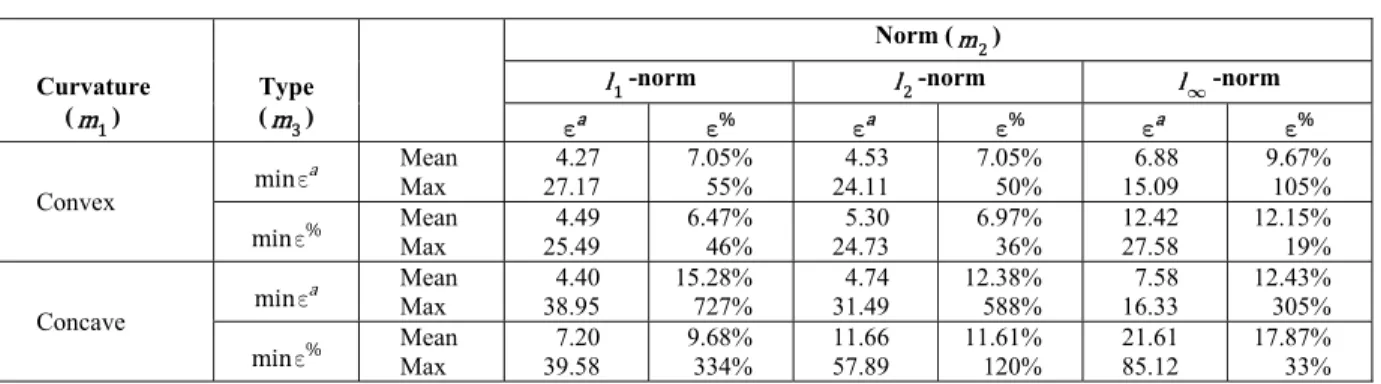
Analyzing the error indexes, it can be noticed that the strategies with concave curvature yield a worse fit than their convex counterpart: concave, ,m m is worse than convex,m m, for all m and m . Further, the convex strategies that minimize relative error tend to induce a better fit than the convex strate-gies that minimize absolute error: convex,m ,minea
is worse than convex,m ,mine% for all m . The remaining issue is the choice of the error norm m for the strategy convex,m ,mine% . Because the mean errors obtained with the strategy convex, ,l¥
%
mine are relatively high, the remaining choices are l and l . The strategy convex, ,minl e% was chosen for the computational experiments because l produced lower mean error in absolute and relative terms.
Computational Analysis
The MILP and MICP formulations were pro-grammed in AMPL and solved with CPLEX 11 in an Intel Core 2 Quad at 2.93 GHz, running on a 64-bit Linux workstation, with 4 GB of RAM. An MINLP formulation was obtained from MICP by imposing the pressure balance at equality on the flow lines (i.e., replacing inequality (13n) with an equality) was also programmed in AMPL, but solved with the global solver SCIP 3.0 (Achterberg et al., 2008; Achterberg, 2009) on the same workstation. All experiments ran with a time limit of 10 000 seconds (≈2.8 hours).
Table 2: Error analysis of the (concave and convex) quadratic approximations.
Curvature (m )
Type (m )
Norm (m )
l -norm l -norm l¥-norm
a
e e% ea e% ea e%
Convex min
a
e Mean Max 27.17 4.27 7.05% 55% 24.11 4.53 7.05% 50% 15.09 6.88 9.67% 105%
%
mine Mean Max 25.49 4.49 6.47% 46% 24.73 5.30 6.97% 36% 12.42 27.58 12.15% 19%
Concave min
a
e Mean Max 38.95 4.40 15.28% 727% 31.49 4.74 12.38% 588% 16.33 7.58 12.43% 305%
%
A Mixed-Integer Convex Formulation for Production Optimization of Gas-Lifted Oil Fields with Routing and Pressure Constraints 449 The lift-gas availability was varied in three
different situations: the compressor has full capacity in the first case (High), half in the second (Medium), and only the capacity for maximizing the production of a single well (Low). This variation in compressing capacity aims to assess the relative performance of the formulations under disparate operational conditions.
The quality of approximation varies according to two different resolutions: a moderate number of polytopes in the PWL functions (Moderate), and a considerably high number of polytopes (Fine). The Moderate resolution has 18 polytopes (squares) for the WPC curve (6 breakpoints for injection rate, and 3 for manifold pressure), and 125 polytopes (cubes) for the pressure-drop function (5 breakpoints for each phase flow). The Fine resolution has 66 poly-topes (squares) for WPC curves (11 breakpoints for injection rate, and 6 for manifold pressure), and 103 polytopes (cubes) for pressure-drop functions (10 breakpoints for each phase flow). The goal for vary-ing the resolution is to evaluate the trade-off between the quality of approximation and the relative performance of the formulations.
For the sake of simplicity, we assume that
n =
, the number of breakpoints for qin is
,
n m =K
and the number of breakpoints for pm is |n m, |=R in the well-production functions, which imply n m, = K- R- for all m and
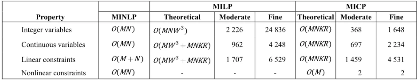
n. Further, the number of breakpoints in each dimension (oil, gas, and water) for Δpm is W which implies m =W - for allm. Table 3 gives the size of the conceptual MINLP, MILP and MICP formulation as a function of these parameters, along with the actual size of the Moderate and Fine instance. The size of the MICP and the MINLP formulation obtained by imposing an equality on the
pressure balance are the same.
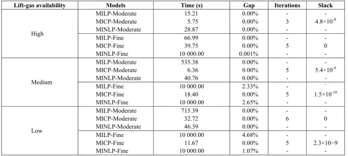
For solving POP m , an iterative process was followed in which the penalty factor was initialized
asm = , and updated asmk+ = mk / , until em became lower than 10-6. Table 4 shows the execution time in seconds and the final dual gap of the solutions obtained with these formulations. For MICP, the table also provides the total number of iterations performed and the maximum slack on the pressure constraint (13n), i.e.,
,
maxïíïïìpm S +Δpm-pm :mÎ ýüïïï.
ï ï
î þ
The computational experiments revealed that the production optimization problem may not be efficiently solved with the MILP and MINLP formulation:
The MILP formulation reached the global optimum with the Moderate resolution for all compression capacities. With a Fine resolution, it was solved to optimality for high capacity, but failed to close the primal-dual gap with medium and low compression capacities.
The MINLP formulation was solved more efficiently than the MILP formulation for the Moderate resolution, but the primal-dual gap could not be closed with the Fine resolution.
On the other hand, globally optimal solutions were found relatively quickly using the MICP formulation for all instances, arguably due to the gradient information provided by the convex-quadratic approximations and the reduced number of binary variables.
It can also be noticed that the approximation of
the pressure-drop equation, Δpm=pm-pm,S with inequality (13n) was very accurate. This behavior corroborates the hypothesis that this inequality is binding, with the slack in the inequality being essentially zero.
Table 3: MILP and MICP formulation size.
Property
MILP MICP
MINLP Theoretical Moderate Fine Theoretical Moderate Fine
Integer variables O MN O MNW 2 226 24 836 O MNKR 368 1 648
Continuous variables O MN O MW +MNKR 962 4 248 O MNKR 697 2 234
Linear constraints O M N+ O MW +MNKR 1 707 6 529 O MNKR 1 459 4 531
Table 4: Computational time of formulations.
Lift-gas availability Models Time (s) Gap Iterations Slack
High
MILP-Moderate 15.21 0.00% - -
MICP-Moderate 5.75 0.00% 3 4.8×10⁻⁸
MINLP-Moderate 28.87 0.00% - -
MILP-Fine 66.99 0.00% - -
MICP-Fine 39.75 0.00% 5 0
MINLP-Fine 10 000.00 0.001% - -
Medium
MILP-Moderate 535.38 0.00% - -
MICP-Moderate 6.36 0.00% 5 5.4×10⁻⁹
MINLP-Moderate 40.76 0.00% - -
MILP-Fine 10 000.00 2.33% -
-MICP-Fine 18.40 0.00% 5 1.5×10⁻¹⁰
MINLP-Fine 10 000.00 2.65% - -
Low
MILP-Moderate 715.39 0.00% - -
MICP-Moderate 32.72 0.00% 6 0
MINLP-Moderate 46.39 0.00% - -
MILP-Fine 10 000.00 4.68% - -
MICP-Fine 11.67 0.00% 5 2.3×10⁻⁹
MINLP-Fine 10 000.00 1.07% - -
Simulation Analysis
This section presents an approach for analyzing and reducing mean errors between the values of process variables calculated with the simulator and their predictions obtained with the MILP and MICP formulations. The solutions obtained with the MICP and MINLP formulation were essentially identical. This approach called off-line simulator-optimizer-application loop is shown in Figure 2.
Figure 2: Off-line simulator-optimizer-application loop.
Aiming to reduce the discrepancy between opti-mization models and the process simulation model, the off-line loop applies four steps:
Step 1: The application gives the simulator an initial resolution quality.
Step 2: The nonlinear functions are sampled in
the multi-phase flow simulator.
Step 3: The optimizer receives the sample break-points as inputs and finds a solution providing lift-gas rates, well-manifold routes, flow rates, and pres-sure predictions.
Step 4: The lift-gas rates and well-manifold routes obtained by the optimizer are injected into the simu-lator. Then, the values calculated by the simulator and the optimizer predictions are given as inputs to the application. A mean error is calculated for the cur-rent resolution and the application decides whether a new iteration is necessary for the optimizer predic-tions to match simulator values. If the resolution quality needs to be improved, a new iteration starts from step 1.
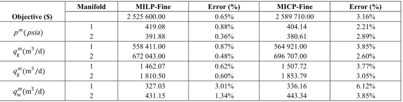
The simulation analysis evaluated the mean errors of the scenario with low compression capacity for both optimization models (MILP and MICP) con-sidering two resolution iterations: Moderate and Fine resolutions. Tables 5 and 6 present the simulation values and the relative errors of the optimization model predictions, for Moderate and Fine resolutions respectively. The MILP and MICP formulations produced the same well-manifold routes. The differ-ences arise in the multiphase flows handled by the manifolds and their pressures.
at-A Mixed-Integer Convex Formulation for Production Optimization of Gas-Lifted Oil Fields with Routing and Pressure Constraints 451 tributed to an insufficient number of breakpoints to
represent the nonlinear characteristics of well-per-formance and pressure-drop curves.
According to Table 6, the simulator-relative er-rors of the Fine resolution are relatively low when compared to the Moderate resolution. The mean of the mean errors is 1.02% for MILP-Fine and 3.5% for MICP-Fine. Once the resolutions of the MILP and MICP are improved, the simulator-relative errors decrease and good solutions are reached with both formulations.
The MILP-Fine formulation is more precise and achieves a representation quite similar to the real process according to the simulator.
The computational and simulation analyses elicit the following remarks:
Performance: The computational analysis shows that an improvement in the resolution quality has a significant impact on the performance of the MILP formulation. When the lift-gas delivered by the com-pression unit is constrained to medium or low, the MILP formulation could not reach the global opti-mum with the Fine resolution. On the other hand, an
improvement in the resolution quality does not slow down the MICP formulation significantly. This result was expected since the MICP formulation has the advantage of being more compact—the three-dimen-sional functions (pressure drops) are approximated with a quadratic function.
Process Representation: The analysis indi-cates that both MILP and MICP formulations reach better solutions when the approximation resolution is improved (the number of sampled breakpoints is in-creased). In order to reduce the optimizer prediction errors, some iterations of the off-line simulator-opti-mizer-application loop will be necessary to deter-mine a sufficient number of breakpoints for a satis-factory approximation of the nonlinear functions.
Extrapolation of the Sampled Region: The MICP formulation was bound to the same sampled region of the MILP formulation. However, the MICP approach is able to extrapolate out of the sampled region within which the convex-quadratic approxi-mation was fitted. It might not be a good approxima-tion, but at least it gives us a lead about the existence of better operating points.
Table 5: Comparison between decision variables of MILP and MICP with moderate approximation.
Objective ($)
Manifold MILP-Moderate Error (%) MICP-Moderate Error (%)
2 277 110.00 5.08% 2 335 690.00 2.66%
m
p psia 1 391.77 4.01% 386.06 5.61% 2 383.41 1.88% 371.92 1.06%
gm m d/
q 1 2 479 023.00 629 903.00 10.26% 1.00% 495 578.00 641 826.00 7.89% 1.50%
om m d/
q 1 2 1 307.70 1 693.28 8.08% 9.30% 1 341.24 1 742.16 12.38% 5.72%
w m d/ m
q 1 316.73 8.63% 322.10 2 349.76 28.51% 459.96 31.23% 10.86%
Table 6: Comparison between decision variable of MILP and MICP with fine approximation.
Objective ($)
Manifold MILP-Fine Error (%) MICP-Fine Error (%)
2 525 600.00 0.65% 2 589 710.00 3.16%
m
p psia 1 419.08 0.88% 404.14 2.21% 2 391.88 0.36% 380.61 2.89%
gm m d/
q 1 2 558 672 411.00 0.87% 043.00 0.48% 564 696 921.00 3.85% 707.00 2.60%
gm m d/
q 1 1 2 1 462.07 0.62% 1 810.50 0.60% 1 507.72 3.77% 853.79 3.05%
w m d/ m
SUMMARY
This work proposed a mixed-integer convex programming formulation for oil production opti-mization of gas-lifted oil fields subject to opera-tional, routing, and pressure constraints. The MICP formulation arises from the piecewise-linearization of the well-production functions and their composi-tion with convex-quadratic approximacomposi-tion funccomposi-tions of the pressure drops. Besides being relatively com-pact, the convexity of the MICP formulation allows for optimization solvers to reach globally optimal solutions. The piecewise-linear models arose from the convex combination of well-production points sampled in the domain of lift-gas injection and mani-fold pressure, whereas the convex-quadratic models were obtained by solving a semi-definite program for fitting the model to pressure-drop points sampled from a multiphase-flow simulator.
A computational analysis performed in a syn-thetic oil field modeled in a multiphase-flow simula-tor showed that the MICP formulation is more efficient than the MILP and MINLP formulation.
A simulation analysis performed in the same oil field showed that the MILP and MICP formulations reach better solutions when the approximation reso-lution is improved. Although the MILP formulation is more precise, it might not be efficient when the approximation resolution is fine. The MICP formula-tion approximates the three-dimensional funcformula-tions (pressure drops) with a single quadratic function re-sulting in a more compact formulation. This MICP approach has the advantage of not being significantly slowed down when the resolution quality is im-proved.
Future research directions include:
the design of more detailed models for pressure drop, possibly including temperature and outlet pres-sure in the pipelines;
the development of piecewise-convex models, which could more precisely approximate complex functions while being more compact than piecewise-linear models; and
the integration with compressor scheduling models (Camponogara et al., 2011; Camponogara et al., 2012).
ACKNOWLEDGMENTS
This work was funded in part by a research contract with Petróleo Brasileiro S.A. (Petrobras).
NOMENCLATURE
Parameters
N number of wells M number of manifolds
max i
q maximum lift-gas rate which represents the compressor capacity
,min in
q lift-gas injection lower bound ,max
in
q lift-gas injection upper bound ,S
m
p nominal pressure for separator
,L n
q lower bound on well flow rate
,U n
q upper bound on well flow rate
,min m
q minimum manifold flow rate ,max
m
q maximum manifold flow rate ,max
m
p maximum manifold pressure
Sets
set of wells set of manifolds
m
subset of wells that can be connected to manifold m
n
manifolds that well n can send its production set of phase flows set of polytopes
V P set of vertices of a polytope set of all vertices
P v set of polytopes that contain vertex v
, n m
breakpoints for the lift-gas rate when well n is connect to manifold m
, n m
manifold pressure
breakpoints when well n is connected to manifold m ,
n m
set of polytopes with vertices in n m, ´n m,
, i, r
n m q p
subset of polytopes that contain vertex q pi, r m
A Mixed-Integer Convex Formulation for Production Optimization of Gas-Lifted Oil Fields with Routing and Pressure Constraints 453 o g w, ,
mk k k
subset of polytopes containing vertex
o, g, w k k k m
set of all vertices in the domain of the pressure drop function
Variables
in
q
gas injection rate for well n ny well n activation ,
n m
z connection of well n to manifold m
,
n m h
q flow of phase h from well n to manifold m
m
q total multiphase flow handled by manifold m
m
p pressure in manifold m v
λ weight for vertex v in a piecewise-linear
approximation P
y polyhedron selection in piecewise-linear
approximation
i, r
, ,
n m q p
λ weighting variable for vertex i, r
q p ,
n m P
d binary variable indicating that a polytope P is active ,
n m
q approximation of well production
Δpm approximation of pressure drop in the flowline of manifold m
m
e excess variable for approximation error of pressure drop
o g w, ,
Ωmk k k weighting variable for vertex
o, g, w
k k k m
y auxiliary variable indicating that a manifold m is receiving production
m P
y binary variable indicating that a polytope PÎm is active
Functions
g objective profit function
c
objective cost function ,n m
q production function of well n when connected to manifold m
Δpm pressure drop in the flow line of manifold m
REFERENCES
Achterberg, T., SCIP: Solving constraint integer pro-grams. Mathematical Programming Computation, 1(1), pp. 1-41 (2009).
Achterberg, T., Berthold, T., Koch, T. and Wolter, K., Constraint integer programming: A new approach to integrate CP and MIP. In Proceedings of the 5th International Conference on Integration of AI and OR Techniques in Constraint Programming for Combinatorial Optimization Problems, pp. 6-20 (2008).
Alarcón, G. A., Torres, C. F. and Gómez, L. E., Global optimization of gas allocation to a group of wells in artificial lift using nonlinear con-strained programming. ASME Journal of Energy Resources Technology, 124 (4), pp. 262-268 (2002).
Beggs, D. and Brill, J., A study of two-phase flow in inclined pipes. Journal of Petroleum Technology, 25(5), pp. 607-617 (1973).
Bieker, H. P., Topics in Offshore Oil Production Optimization Using Real-time Data. Ph.D. Thesis, Norwegian University of Science and Technology (2007).
Boyd, S. and Vandenberghe, L., Convex Optimization. Cambridge University Press (2004).
Buitrago, S., Rodruiguez, E. and Espin, D., Global optimization techniques in gas allocation for continuous flow gas lift systems. In Proceedings of the SPE Gas Technology Symposium (1996). Camponogara, E. and Nakashima, P. H. R., Solving
a gas-lift optimization problem by dynamic pro-gramming. European Journal of Operational Research, 174(2), pp. 1220-1246 (2006).
Camponogara, E. and Conto, A. M., Lift-gas alloca-tion under precedence constraints: MILP formula-tion and computaformula-tional analysis. IEEE Transac-tions on Automation Science and Engineering, 6(3), pp. 544-551 (2009).
Camponogara, E., Castro, M. P., Plucenio, A. and Pagano, D. J., Compressor scheduling in oil fields: Piecewise-linear formulation, valid inequalities, and computational analysis. Optimization and En-gineering, 12, pp. 153-174 (2009).
Camponogara, E., Nazari, L. F. and Meneses, C., A revised model for compressor design and sched-uling in gas-lifted oil fields. IIE Transactions, 44, pp. 342-351 (2012).
optimization for optimal lift-gas allocation with well-separator routing. European Journal of Op-erational Research, 217, pp. 222-231 (2012). Codas, A., Campos, S. R. V., Camponogara, E.,
Gunnerud, V. and Sunjerga, S., Integrated pro-duction optimization of oil fields with pressure and routing constraints: The Urucu field. Com-puters & Chemical Engineering, 46, pp. 178-189 (2012).
Gunnerud, V. and Foss, B., Oil production optimiza-tion–a piecewise linear model, solved with two decomposition strategies. Computers & Chemical Engineering, 34(11), pp. 1803-1812 (2010). Kosmidis, V. D., Perkins, J. D. and Pistikopoulos, E.
N., Optimization of well oil rate allocations in petroleum fields. Industrial & Engineering Chem-istry Research, 43(14), pp. 3513-3527 (2004). Litvak, M. and Darlow, B., Surface network and well
tubing-head pressure constraints in compositional simulation. In Proceedings of the SPE Reservoir Simulation Symposium, San Antonio, USA (1995). Litvak, M. L., Clark, A. J., Fairchild, J. W., Fossum,
M. P., MacDonald, C. J. and Wood, A. R. O., In-tegration of Prudhoe Bay surface pipeline net-work and full field reservoir models. In Proceed-ings of the SPE Annual Technical Conference and Exhibition, San Antonio, USA (1997). Löfberg, J., YALMIP: A toolbox for modeling and
optimization in MATLAB. In Proceedings of the IEEE International Symposium on Computer-Aided Control System Design, Taipei, Taiwan (2004).
Misener, R., Gounaris, C. E. and Floudas, C. A., Global optimization of gas lifting operations: A comparative study of piecewise linear formula-tions. Industrial & Engineering Chemistry Re-search, 48(13), pp. 6098-6104 (2009).
Moisés, G. V., Rolim, T. A. and Formigli, J. M., Gedig: Petrobras corporate program for digital integrated field management. In Proceedings of the SPE Intelligent Energy Conference and Exhi-bition, Amsterdam, The Netherlands (2008). Peaucelle, D., Henrion, D., Labit, Y. and Taitz, K.,
User’s guide for SeDuMi interface 1.04. Techni-cal Report, LAAS, CNRS (2002).
Silva, T. L., Codas, A. and Camponogara, E., A com-putational analysis of convex combination models for multidimensional piecewise-linear approxima-tion in oil producapproxima-tion optimizaapproxima-tion. In Proceedings of the IFAC Workshop on Automatic Control in Offshore Oil and Gas Production, Trondheim, Norway (2012).
Silva, T. L., Camponogara, E., A computational analysis of multidimensional piecewise-linear models with applications to oil production opti-mization. European Journal of Operational Re-search, 232(3), pp. 630-642 (2014).
Vielma, J. P., Ahmed, S. and Nemhauser, G., Mixed-integer models for nonseparable piecewise linear optimization: unifying framework and extensions. Operations Research, 58(1), pp. 303-515 (2010). Williams, C. and Webb, T., Shell strives to make
smart fields smarter. Society of Petroleum Engi-neers (2007).
APPENDIX
SEMI-DEFINITE REFORMULATIONS
The strategies for finding quadratic approxima-tions are a variation of problem CF given in Equa-tion (12), which can be easily recast as a standard SDP by replacing the objective with:
min k
kÎ
j
å
(A1a)
and introducing the inequalities:
, ,
,
Δ Δ ,
Δ
m k m k
k p m kp k k
p
-j £ £j " Î (A1b)
The l¥- norm for approximation error can be handled in a similar manner by simple manipulation of problem CF . It suffices to introduce inequality (A1b), introduce the inequalities j £ j " Îk , k , and replace the objective withminj.
The representation of the square of the approxi-mation error (l -norm) requires the use of Schur complement since quadratic functions are not explic-itly allowed in SDP. The synthesis of convex-quadratic models using the l -norm of relative errors can be cast as an SPD program:
, ,
min
m m m k
Q c kÎ
j
å
bA Mixed-Integer Convex Formulation for Production Optimization of Gas-Lifted Oil Fields with Routing and Pressure Constraints 455
,
( )
, , ,Δ
s.t.: pm k m k TQm m k Tm m k cm ,
k
= + +
" Î
q q b q
(A2b) , , , , , ,
Δ Δ
Δ
Δ Δ
Δ , m k m k m k m k m k k T m k p p I p p p p k
é æç ö÷ù
ê ç - ÷÷ú
ê çç ÷÷ú
êæ ö çç ÷÷ú
êççê - ÷÷ è øúú ÷
ç ÷ j
çê ÷ ú
ç ÷
êçè ÷ø ú
ê ú
ë û
" Î
(A2c)
m mT
Q =Q (A2d)
, ,
m m m
Q Î ´ b δ c Î (A2e)
According to Schur complement, Eq. (A2c) is equivalent to: , , , , , , , , ,
Δ Δ Δ Δ
Δ Δ
Δ Δ
Δ
m k m k
m k m k
k m k m k
m k m k
k T
k m
p p I p p
p p
p p
p
-æ ö÷ æ ö÷
ç ÷ ç ÷
ç ÷ ç ÷
ç - ÷ ç - ÷
ç ÷ ç ÷
ç ÷ ç ÷
j -ç ÷÷ ç ÷÷
ç ÷ ç ÷
ç ÷ ç ÷
ç ÷ ç ÷
ç ÷ ç ÷
è ø è ø
æ ö÷
ç ÷
ç ÷
ç - ÷
ç ÷
ç ÷
j ³ç ÷÷
ç ÷ ç ÷ ç ÷ ç ÷ è ø
Notice that the fitting of concave-quadratic func-tions is achieved by using Qm as the condition on the Hessian. Approximations that minimize abso-lute error are obtained by eliminating the
denomina-tor Δpm k, from the equations that calculate error.
The gas-flow rates are of the order of 6 and
when squared reach values of the order of a trillion of m /d, which are far larger than the water- and oil-flow rates. Thus, normalization of the flow rates was required before using the SDP solver to find a
quadratic approximation Δ .pm
The normalization is obtained with a diagonal matrixTm as follows:
,o ,g ,w 0 0 0 0 0 0 m m m m T T T T
ˆm=Tm m
q q
where ˆqm is the normalized multiphase-flow rate and Tm,o Tm,g,Tm,w is the maximum oil-flow rate (gas-flow and water-flow rate). Solving problem
CF using the normalized flow-rates ˆqm yields a normalized quadratic approximation function given
by Q ˆ , ˆbm m, and cˆm. Thus,
( )
( )
( )
(
)
(
)
(
)
( )
( )
( )
( )
( )
mm m m m m m
m m m m m m m m m
m m m m m m m m m
T
m m m m m m
p Q c
T Q T T c
T Q T T c
Q c
ˆ ˆ
ˆ ˆ ˆ ˆ
ˆ ˆ ˆ ˆ ˆ Δ ˆ T T T T
T T T
T T = + + = + + = + + = + +
q q b q
q q b q
q q b q
q q b q
by defining,Qm=T mT Q Tˆm m, bm= T mT bˆm , and ˆ
=
m m