Constraints on methane emissions in North America from future geostationary remote-sensing measurements

(1)

www.atmos-chem-phys.net/16/6175/2016/ doi:10.5194/acp-16-6175-2016

Constraints on methane emissions in North America from future

geostationary remote-sensing measurements

Nicolas Bousserez1, Daven K. Henze1, Brigitte Rooney1, Andre Perkins1,a, Kevin J. Wecht3, Alexander J. Turner3, Vijay Natraj2, and John R. Worden2

1_{Department of Mechanical Engineering, University of Colorado, Boulder, CO, USA} 2_{Jet Propulsion Laboratory, California Institute of Technology, Pasadena, CA, USA} 3_{School of Engineering and Applied Sciences, Harvard University, Cambridge, MA, USA} a_{now at: Department of Atmospheric Sciences, University of Washington, Seattle, WA, USA} Correspondence to:Nicolas Bousserez (nicolas.bousserez@colorado.edu)

Received: 21 April 2015 – Published in Atmos. Chem. Phys. Discuss.: 10 July 2015 Revised: 25 March 2016 – Accepted: 15 April 2016 – Published: 20 May 2016

Abstract.The success of future geostationary (GEO) satel-lite observation missions depends on our ability to design instruments that address their key scientific objectives. In this study, an Observation System Simulation Experiment (OSSE) is performed to quantify the constraints on methane (CH4) emissions in North America obtained from shortwave

infrared (SWIR), thermal infrared (TIR), and multi-spectral (SWIR+TIR) measurements in geostationary orbit and from future SWIR low-Earth orbit (LEO) measurements. An effi-cient stochastic algorithm is used to compute the information content of the inverted emissions at high spatial resolution (0.5◦×0.7◦) in a variational framework using the GEOS-Chem chemistry-transport model and its adjoint. Our results show that at sub-weekly timescales, SWIR measurements in GEO orbit can constrain about twice as many independent flux patterns than in LEO orbit, with a degree of freedom for signal (DOF) for the inversion of 266 and 115, respectively. Comparisons between TIR GEO and SWIR LEO configu-rations reveal that poor boundary layer sensitivities for the TIR measurements cannot be compensated for by the high spatiotemporal sampling of a GEO orbit. The benefit of a multi-spectral instrument compared to current SWIR prod-ucts in a GEO context is shown for sub-weekly timescale constraints, with an increase in the DOF of about 50 % for a 3-day inversion. Our results further suggest that both the SWIR and multi-spectral measurements on GEO orbits could almost fully resolve CH4 fluxes at a spatial resolution of

at least 100 km×100 km over source hotspots (emissions >4×105kg day−1). The sensitivity of the optimized

emis-sion scaling factors to typical errors in boundary and initial conditions can reach 30 and 50 % for the SWIR GEO or SWIR LEO configurations, respectively, while it is smaller than 5 % in the case of a multi-spectral GEO system. Over-all, our results demonstrate that multi-spectral measurements from a geostationary satellite platform would address the need for higher spatiotemporal constraints on CH4emissions

while greatly mitigating the impact of inherent uncertainties in source inversion methods on the inferred fluxes.

1 Introduction

Methane (CH4) plays a key role in both atmospheric

chem-istry composition and climate. With a radiative forcing rel-ative to preindustrial times that is one-third that of carbon dioxide, CH4 is the second most important greenhouse gas

(Myhre and Shindell, 2013). Furthermore, as a precursor to tropospheric ozone, CH4also impacts surface-level air

qual-ity (Fiore et al., 2002; West et al., 2006; West and Fiore, 2005) and crops (e.g., Shindell et al., 2012), and contributes to ozone radiative forcing (e.g., Fiore et al., 2008). Con-siderable uncertainty remains in our understanding of CH4

sources (e.g., Dlugokencky et al., 2011; Kirschke et al., 2013), which include emissions from coal, wetlands, live-stock, landfills, biomass burning, geologic seepage, and leaks from the production and distribution of natural gas.

Although there is a growing interest in using CH4

(2)

ad-dress current air quality and global warming challenges (e.g., West et al., 2012), the lack of confidence in the available CH4emission estimates remains a problematic limitation to

the design of efficient environmental policies. Indeed, recent studies showed discrepancies of up to a factor of 2 between bottom-up inventories and top-down inversions using atmo-spheric CH4 concentration observations (Katzenstein et al.,

2003; Kort et al., 2008; Xiao et al., 2008; Karion et al., 2013; Miller et al., 2013; Wecht et al., 2012, 2014a; Caulton et al., 2014; Turner et al., 2015). Extrapolation of local emis-sion characteristics to larger areas and/or the use of proxy data (e.g., energy consumption, emission ratios applied to co-emitted species) are the main sources of error in bottom-up methods. On the other hand, top-down approaches us-ing space-based measurements of CH4from low-Earth orbit

(LEO) platforms allow a global spatial coverage within 1 to 6 days but at the same local time. However, as CH4emissions

can exhibit significant diurnal cycles, e.g., over wetland or boreal peatland (Morin et al., 2014; Gazovic et al., 2010), such temporal undersampling may affect our ability to ac-curately quantify those fluxes. More generally, insufficient observational coverage and the diffusive nature of transport considerably reduce our ability to spatially resolve grid-scale emissions from space.

Geostationary (GEO) remote-sensing measurements would alleviate the above-mentioned shortcomings by providing an almost continuous monitoring and complete spatial coverage of CH4 concentrations within the field

of view. Previous studies have already demonstrated the potential of column-integrated trace gas measurements from geostationary satellites to constrain surface fluxes at regional scale, from single mega-city emissions down to power plant sources (Polonsky et al., 2014; Rayner et al., 2014). The GEOstationary Coastal and Air Pollution Events (GEO-CAPE) mission (Fishman et al., 2012) was recommended by the National Research Council’s Earth Science Decadal Survey in order to improve our understanding of both coastal ecosystems and air quality from regional to continental scale. Its aim is to enable multiple daily observations of key atmospheric and oceanic constituents over North and South America from a GEO platform. For air-quality applications, such high-spatial and high-temporal-resolution measurements would enable source estimates of air-quality pollutants and climate forcers and development of effective emission-control strategies at an unprecedented level of confidence. In order to provide more flexibility and to minimize the cost and risk of the mission, the concept of a phased implementation that would launch remote-sensing instruments separately on commercial host spacecrafts has been adopted. The first phase will consist of the launching of the Tropospheric Emissions: Monitoring of Pollution (TEMPO) instrument circa 2019 (Chance et al., 2013), which will provide GEO hourly measurements of ozone and precursors as well as aerosols over greater North America (from Mexico City to the Canadian tar sands, and from the

Atlantic to Pacific oceans). For the second phase, which aims at completing GEO-CAPE’s mission requirements by including measurements of important drivers of climate and air quality such as CH4, CO, and ammonia (Zhu et al., 2015),

a rigorous instrument design study is critical to achieve the mission’s scientific objectives within its budget constraints.

In this study we perform an Observation System Simu-lation Experiment (OSSE) in order to characterize the con-straints on grid-scale CH4 emissions over North America

provided by different potential GEO-CAPE instrument con-figurations. The simulation consists of a 4D-Var inversion of CH4emissions using the GEOS-Chem chemical-transport

model (CTM) over a 0.5◦×0.7◦ horizontal grid resolution covering North America. In practice, quantifying the infor-mation content of such a high-dimensional problem requires either Monte Carlo simulations or, for linear models, a nu-merical approximation of the inverse Hessian matrix of the 4D-Var cost function (Tarantola, 2005). Although previous studies have used Monte Carlo estimates (e.g., Chevallier et al., 2007; Liu et al., 2014; Cressot et al., 2014), their com-putational cost can be extremely high. Indeed, many per-turbed inversions (typically about 50) are needed, each of them requiring numerous forward and adjoint model integra-tions (iteraintegra-tions) in case the problem is not well conditioned (about 50 iterations for our methane inversion). Alternatively, inverse Hessian approximations based on information from the minimization itself can be employed, but are usually of very low rank (e.g., Meirink et al., 2008; Bousserez et al., 2015). Therefore, most information content analyses in pre-vious trace-gas Bayesian inversion studies have relied on ex-plicit calculations of the inverse Hessian matrix, by either considering a regional domain (e.g., Wecht et al., 2014a) or performing a prior dimension reduction of the control vector (e.g., Wecht et al., 2014b; Turner and Jacob, 2015). However, thus far dimension reduction methods for high-dimensional problems have relied on suboptimal choices for the reduced space, which preclude an accurate and objective quantifica-tion of the spatiotemporal constraints on the optimized emis-sions.

In this study we use a gradient-based randomization al-gorithm to approximate the inverse Hessian of the cost func-tion (Bousserez et al., 2015), which allows us to calculate the posterior errors as well as the model resolution matrix (or av-eraging kernel) of our CH4emission inversion at grid-scale

resolution. Such information is used to evaluate the impact of different instrumental designs (spatiotemporal sampling, ver-tical sensitivity of the measurements) on CH4emission

con-straints. In particular, the potential of CH4retrievals from the

(3)

results of our experiments, where the information content of the inversion is analyzed in detail. A conclusion to this work is presented in the last section of the paper.

2 Inverse method

2.1 4D-Var system and information content

The variational approach to Bayesian inference is the method of choice for high-dimensional problems, since the solution can be computed by iteratively minimizing a cost function instead of algebraically solving for the minimum, which be-comes computationally intractable for high-dimensional sys-tems. Provided the error statistics are all Gaussian, finding the maximum likelihood entails solving the following prob-lem:

arg min

x J (x) (1)

J (x)=1

2(H (x)−y)

T_R−1_{(H (x)}₋_y)

+1

2(x−xb)

T_B−1_(x₋

xb),

wherexbis the prior vector, defined in the control spaceE

of dimensionn,xbelongs toE,yis the observation vector, defined in the observations vector spaceF of dimension p, H:E→F is the forward model operator (also called the observational operator), which associates with any vector in E its corresponding observation inF, and RandBare the covariance matrices of the observation and prior errors with dimension(p×p)and(n×n), respectively. The argument of the minimum of Eq. (1) is called the analysis and is referred to asxa.

When the adjoint of the forward model (HT_{) is available,} the minimum of the cost function J can be found itera-tively using a gradient-based minimization algorithm (Lions, 1971). The gradient of the cost function with respect to the control vectorxcan be written as

∇J (x)=HTR−1(H (x)−y)+B−1(x−xb). (2)

An important result is that if the forward model is ap-proximately linear, the posterior error covariance matrixPa is equal to the inverse of the Hessian of the cost function: Pa=(∇2J )−1(xa)=(B−1+HTR−1H)−1. (3)

This equivalence can be used to compute information con-tent diagnostics prior to performing the inversion. In this study, following Bousserez et al. (2015), the diagonal ele-ments ofPa(error variances) are computed using a random-ization estimate ofHTR−1H. Here an ensemble of 500 ran-dom gradients of the cost function are used, based on the con-vergence of the uniform norm (k.k∞) of the inverse Hessian

approximation. Bousserez et al. (2015) showed that good ap-proximation of both the error variances and the error corre-lations can be obtained using this approach. For the present

study we further validated our method by comparing direct finite-difference estimates of selected diagonal elements of Pa to their stochastic approximations, and found a relative error standard deviation smaller than 10 %.

The model resolution matrix (or averaging kernelA) is defined as the sensitivity of the analysisxa (optimized CH4

emissions) to the truthxt(true emissions):

A≡∂xa ∂xt

. (4)

The model resolution matrix in Eq. (4) can be rewritten in matrix form:

A=I−PaB−1. (5)

SinceBis diagonal in our experiments, Eq. (5) allows us to calculate any element ofAusing

Ai,j =δij− Pa_i,j Bj,j

. (6)

Finally, the degree of freedom for signal (DOF) of the inver-sion is defined as the trace ofA, that is, DOF=P_iAi,i. 2.2 Forward model and prior emissions

The forward model in Eq. (1) includes the GEOS-Chem chemistry-transport model, which relates the CH4emissions

to the 3-D concentration field of atmospheric CH4, and the

satellite observation operator that transforms the CH4

con-centration profiles into their corresponding retrieved profile or columns. The GEOS-Chem simulation used in our exper-iment is described in Wecht et al. (2014a) and Turner et al. (2015). It consists of a nested simulation over North Amer-ica at 0.5◦×0.7◦horizontal resolution and 72 vertical levels, driven by offline meteorological data provided by GEOS-5 reanalysis from the NASA Global Modeling and Assimila-tion Office (GMAO). Boundary condiAssimila-tions for the nested do-main are used every 3 h from a global 4◦×5◦GEOS-Chem simulation. In the case of profile assimilation (multi-spectral instrument), the application of the measurement averaging kernels to the model profiles can be written as follows: lnzretr=lnza+A(lnzmod−lnza), (7)

wherezretris the profile that would be retrieved if the

mod-eled profile concentrations (zmod) were sounded, andza

rep-resents the prior profile concentrations. In the case ofXCH4 columns assimilation, we obtain (Parker et al., 2011) XCH4=

XCO2 CO2

(a+aT(ωmod−ωa)), (8)

whereωmodis the modeled vertical profile of methane,ωais

the a priori profile,ais the corresponding a priori column

(4)

CO2is the measured vertical column concentration of CO2, andXCO2is a modeled column mixing ratio of CO2. For sim-plicity, we use a single averaging kernel for each instrument. A larger ensemble of averaging kernels describing a poten-tial range of sensitivities is beyond the scope of this study given the computational cost. However, based on knowledge of thermal IR (e.g., TES) and total column (e.g., TROPOMI) retrievals, use of a single averaging kernel is a reasonable approximation as our study is constrained to Northern Hemi-sphere summertime where the temperature and sunlight con-ditions provide a sufficient signal for the present evaluation, and because our study looks at the relative merits of different observing approaches.

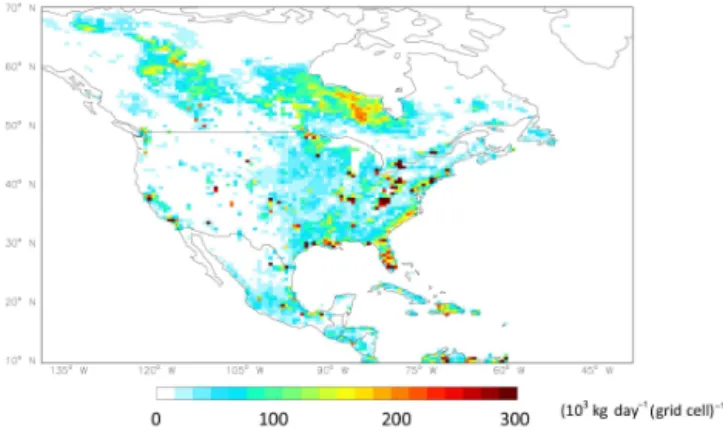
The prior methane emissions we use are from the EDGARv4.2 anthropogenic methane inventory (European Commission, 2011), the wetland model from Kaplan (2002) as implemented by Pickett-Heaps et al. (2011), the GFED3 biomass burning inventory (van der Werf et al., 2010), a ter-mite inventory and soil absorption from Fung et al. (1991), and a biofuel inventory from Yevich and Logan (2003). Fig-ure 1 shows the total average daily prior methane emissions for the entire North America nested domain. Strong hotspots of CH4sources clearly appear over the Canadian wetlands,

the Appalachian Mountains (an extensive coal mining area) and densely urbanized areas (e.g., southern California and the eastern coast). Following previous assessments of the range of the prior error (Wecht et al., 2014a; Turner et al., 2015), we assume a relative prior standard error of 40 % for our bottom-up emission inventory in every grid cell. This re-sults in a 2.9 Tg month−1 _{uncertainty in the total emission}

budget over North America, a magnitude comparable to the correction to the prior budget found in the inversion of Turner et al. (2015) of 2.3 Tg month−1_{. We assume no prior spatial}

error correlations, which means that the matrixBin Eq. (1) is diagonal. Accurately defining error correlations in bottom-up inventories is a challenging problem due to the sparsity of available flux measurements, and is beyond the scope of our study. However, it is likely that the diagonal Bassumption made in our study is overly optimistic, which may result in an overestimation of the spatial resolution of the constraints afforded by the satellite measurements. Note that in our setup one emission scaling factor is optimized per grid cell; there-fore, the temporal variability of the emissions is assumed to be a hard constraint at scales smaller than the assimilation window.

2.3 Observations and model uncertainties

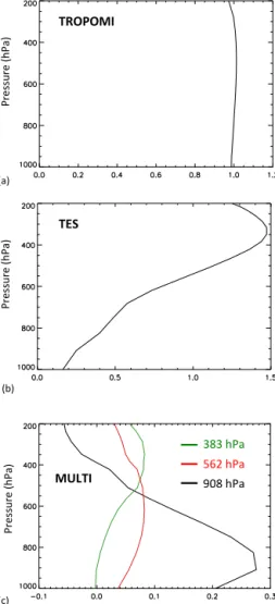
We consider several instrument configurations for our study, which are associated with different vertical sensitivities: the future TROPOMI instrument (2016 launch), which will mea-sure in the shortwave infrared (SWIR); the Tropospheric Emission Spectrometer (TES) V005 Lite product (Worden et al., 2012) (http://tes.jpl.nasa.gov/data/), which consists of CH4 vertical profile retrievals from thermal infrared (TIR)

Figure 1.Total daily average prior methane emissions for the nested North America domain (0.5◦×0.7◦).

measurements at 7.58–8.55 µm; and a hypothetical multi-spectral CH4profile retrieval, which allows us to capture a

signal in the boundary layer. Since the DOF for the TES re-trievals is less than 2, we use a pressure-weighted TESXCH4 column instead of the retrieved CH4 profiles. The

averag-ing kernel for the TROPOMI configuration is taken from the Greenhouse gases Observing SATellite (GOSAT) Proxy XCH4 v3.2 retrieval described by Parker et al. (2011) (avail-able from http://www.leos.le.ac.uk/GHG/data/), which con-sists of CH4 column mixing ratios (XCH4) obtained from SWIR measurements near 1.6 µm. As noted in Wecht et al. (2014b), the difference between the TROPOMI and GOSAT retrievals are of little consequence, as the averaging kernel for SWIR observations is near unity in the troposphere in any case. The multi-spectral averaging kernel is derived by first combining the Jacobians (or sensitivities) of the mod-eled radiances to methane concentrations from the 1.6 and 8 µm bands. Both the TES and GOSAT retrievals also si-multaneously estimate interferences such as clouds, albedo, emissivity, temperature, and H2O. The effects of these

in-terferences can be included by further combining their cor-responding Jacobians with the methane Jacobians (e.g., Wor-den et al., 2004; Kulawik et al., 2006; Butz et al., 2010). Con-straints for methane and the other radiative interferences are described in Worden et al. (2012) and Parker et al. (2011). The combination of these Jacobians and constraints are then used to calculate the averaging kernel. The methane compo-nent of the resulting multi-spectral, multi-species averaging kernel is then used for this study. The effect of the interfer-ences with this simultaneous retrieval approach is to reduce the overall sensitivity to methane but improve the posteriori errors. A proof of concept for combining near-IR and IR-based methane estimates to derive a lower tropospheric esti-mate is discussed in Worden et al. (2015) using GOSAT and TES profile retrievals.

(5)

Pres

su

re

(hP

a

)

Pres

su

re

(hP

a

)

908 hPa

383 hPa

562 hPa

(a)

(c)

TROPOMI

MULTI

Pres

su

re

(hP

a

)

TES

(b)

Figure 2.Averaging kernels for the different instrument configu-rations:(a)TROPOMI column averaging kernel;(b)TES column averaging kernel;(c)multi-spectral averaging kernels at three pres-sure levels: 908, 562 and 383 hPa.

retrieval. The TROPOMI retrieval sensitivity is nearly uni-form throughout the troposphere, with averaging kernel val-ues close to 1. The TES retrieval is mostly sensitive to CH4

concentrations in the upper troposphere, with a peak of the column averaging kernel around 300 hPa. The multi-spectral profile retrieval shows a distinct signal in the boundary layer, with weaker sensitivities above.

Observation and model transport errors are assumed to be independent and therefore added in quadrature to define the error covariance matrixRin Eq. (1). Observational error standard deviations for TROPOMI XCH4 columns are uni-formly set to 12 ppb, within the range of values reported for GOSAT in Parker et al. (2011). For the TES retrievals, the profile error covariance matrix is averaged vertically using pressure-weighted functions to obtainXCH4 column errors, as described in Connor et al. (2008). This results in a 0.5–2 % (or 10–40 ppb) standard error deviation for the TES columns

(Worden et al., 2012). For the multi-spectral retrievals, a ver-tically resolved error covariance matrix is used. The error covariance for the multi-spectral retrieval is derived along with the averaging kernel using the approach described in Fu et al. (2013) and references therein. The Jacobians for CH4and other trace gases affecting the observed radiances,

from the near-IR and thermal IR, are combined along with noise estimates for both spectral regions that are based on TES and GOSAT radiances. Because we assume that inter-ferences such as albedo, emissivity, and H2O are jointly

es-timated, the uncertainties from these interferences are also included in the resulting observation error matrix. The re-sulting pressure-weighted columnXCH4 error standard de-viation is similar to the one obtained for GOSAT retrievals (∼12 ppb).

As shown by Locatelli et al. (2013), taking into account transport errors is critical in order to mitigate uncertainties in the inversion, since neglecting them can lead to discrepancies in the posterior estimates of more than 150 % of the prior flux at model grid scale. We estimate model transport error using model–data comparison statistics for North American in situ observations from the NOAA/ESRL surface, tower, and flask network as well as observations from the HIPPO and Cal-Nex measurement campaigns (Turner et al., 2015). Model error standard deviations are set to 46 ppb in the boundary layer and 22 ppb in the free troposphere. Vertical error cor-relations between simulated concentrations are difficult to quantify with the limited observational sampling available in situ. Transport error correlations between the boundary layer and the free troposphere are assumed to be negligi-ble due to the decoupling of the physical processes between those two regions. However, within both the boundary layer and the free troposphere, a model error correlation of one is assumed between all altitude levels, which is a conserva-tive (pessimistic) assumption. Our gradient-based estimates of the inverse Hessian matrix involve generating random per-turbations that follow the observational error statistics (see Sect. 2.1). For the multi-spectral configuration, a singular value decomposition (SVD) is first performed on the verti-cally resolved matrixRin order to generate independent per-turbations (e.g., Bousserez et al., 2015).

In order to assess the relative impact of measurement sen-sitivity versus spatiotemporal sampling on the CH4

(6)

Figure 3.Density of satellite observations (grid cell−1week−1) for LEO (left) and GEO (right) orbits for the nested North America domain (0.5◦×0.7◦) and for the period 1–8 July 2008.

deviation is reduced by multiplying it by the square root of the number of observations.

Finally, contamination by clouds is taken into account for each grid cell by removing a fraction of the total number of observations within that cell that corresponds to the GEOS-5 cloud fraction. The resulting spatial distribution of the obser-vational data density for each satellite configuration (LEO or GEO) is shown in Fig. 3.

3 Results

In the following experiments, we consider the inversion of 30-, 7-, and 3-day grid-scale emission scaling factors over North America. In particular, this means that the spatiotem-poral variability of the methane fluxes (e.g., diurnal cycle and spatial distribution) within each time window is assumed to be known, and only its magnitude is adjusted. The informa-tion content of the inversion is analyzed for four different observational systems:

– a TROPOMI instrument onboard a low-Earth orbit plat-form (TROPOMI_LEO);

– a TROPOMI instrument onboard a geostationary orbit platform (TROPOMI_GEO);

– a TES-like instrument onboard a geostationary orbit platform (TES_GEO);

– a multi-spectral instrument onboard a geostationary or-bit platform (MULTI_GEO).

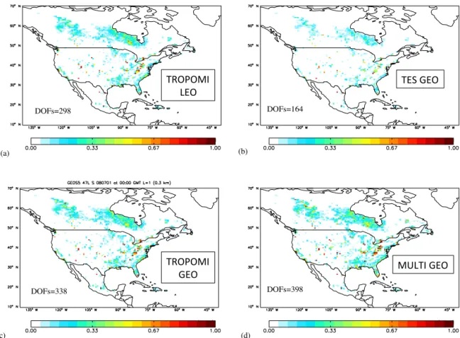
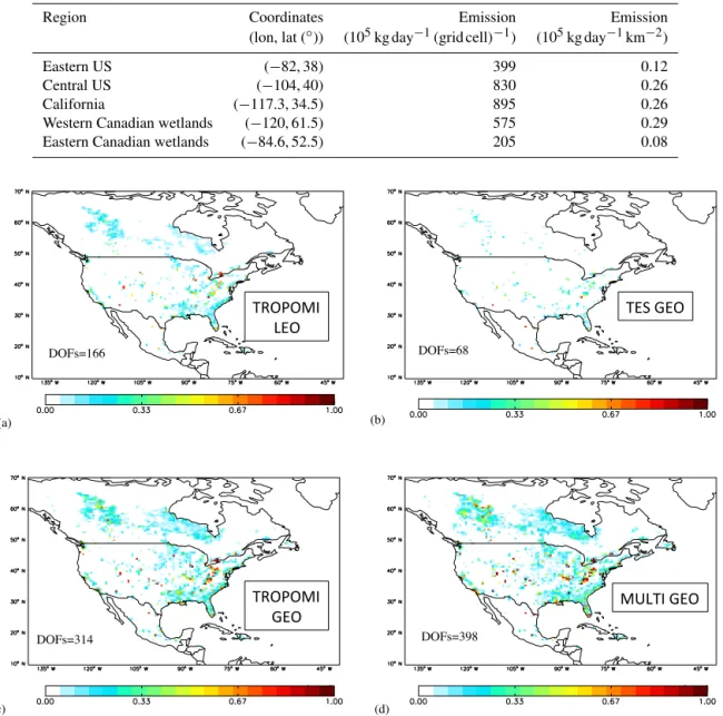
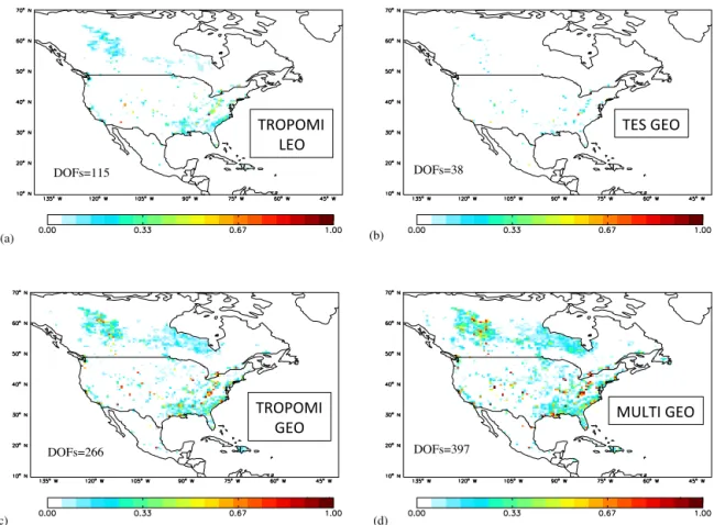
3.1 Error reduction of optimized methane emissions Figures 4, 5, and 6 show the relative error variance reduction in the emission scaling factors for 30-, 7-, and 3-day inver-sions, respectively, for each of the observational configura-tions described above. The DOF, which quantifies the num-ber of pieces of information independently constrained by

the observations, is also indicated. For the monthly inversion, the TROPOMI_LEO, TROPOMI_GEO, and MULTI_GEO configurations show error variance reductions close to 100 % for sparse hotspots over the continent, in particular in the Los Angeles basin, the central US, the Toronto urban area, the Appalachian Mountains, and the northeastern US. The TES_GEO configuration still shows significant observational constraints in those locations, with error variance reductions >70 %. However, overall the error variance reductions af-forded by using a TES-like instrument in geostationary orbit are much smaller than the one obtained from a TROPOMI-like or multi-spectral instrument. In particular, the DOF for the TES_GEO configuration (164) is about half that of the TROPOMI_LEO configuration (298). This demonstrates that using measurements with significant sensitivities to lower-tropospheric concentrations is critical to obtaining surface flux information, even in a geostationary framework with high-frequency temporal sampling. The advantage of the GEO over the LEO configuration is more pronounced when smaller emission timescales are constrained (weekly, 3-day). In particular, the DOF for TROPOMI_LEO varies from 88 to 43 % of the DOF for TROPOMI_GEO between the monthly and 3-day inversions. Similarly, but to a lesser ex-tent, the benefit of a multi-spectral profile observation com-pared to a TROPOMI-like column measurement is most ev-ident when the temporal resolution of the flux inversion is increased, with a DOF ratio between TROPOMI_GEO and MULTI_GEO varying from 84 to 67 % between the monthly and 3-day inversions.

(7)

(a) (b)

(c) (d)

DOFs=298 DOFs=164

DOFs=338 DOFs=398

TROPOMI

LEO

TES GEO

TROPOMI

GEO

MULTI GEO

Figure 4.Relative error variance reduction for a 30-day methane emission optimization (1–30 July 2008) using(a)TROPOMI low-Earth orbit observations (TROPOMI_LEO);(b)GEO-CAPE observations with a TES-like instrument (TES_GEO);(c)GEO-CAPE observations with a TROPOMI-like instrument (TROPOMI_GEO); and(d)GEO-CAPE observations with a multi-spectral instrument (MULTI_GEO). Zero values correspond to emissions with no constraints from observations, while values of one correspond to emissions entirely constrained by observations. The DOF for each inversion, which is the sum of all diagonal elements of the model resolution matrix, is also indicated.

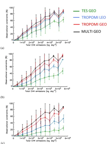
4×105kg day−1grid−1), a multi-spectral instrument in geo-stationary orbit would reduce prior flux error variances by more than 80 % at timescales as small as 3 days. In par-ticular, this could provide valuable information to monitor the variation of CH4 emission hotspot activities between

workweek and weekend. Finally, we note that Turner et al. (2015) obtained a DOF of 39 for a multi-year CH4flux

in-version over North America using GOSAT LEO observa-tions. The much higher DOF (298) obtained for our monthly TROPOMI_LEO inversion clearly demonstrates the impact of spatial sampling when using a TROPOMI LEO config-uration, which will provide roughly 2 orders of magnitude more observations than GOSAT. We also note that in Turner et al. (2015), a prior dimension reduction of the inverse prob-lem was performed to enable an analytical computation of the solution with only 369 control vector elements. Although it is claimed that the aggregation scheme used to define the reduced space is designed to account for prior error corre-lations, the results obtained in Turner et al. (2015) indicate the reduction method is suboptimal (see the interactive dis-cussion of Turner et al., 2015, for more details), which could

result in an underestimation of the DOF. On the other hand, in our case neglecting error correlations in the prior inven-tory may result in an overestimation of the DOF. In the ab-sence of a rigorous methodology to accurately estimate the prior error correlations, the DOFs we derived should there-fore be interpreted with caution, but can provide useful in-sights into the relative magnitude of the constraints afforded by different instruments and orbit configurations. These re-sults also correspond to the limit to which the observational constraints would tend as the effective spatial resolutions of the bottom-up CH4inventories are increased. In relation to

(8)

Table 1.Coordinates of the five locations considered for the rows of the model resolution matrix, with their corresponding emission rate.

Region Coordinates Emission Emission

(lon, lat (◦)) (105kg day−1(grid cell)−1) (105kg day−1km−2)

Eastern US (−82, 38) 399 0.12

Central US (−104, 40) 830 0.26

California (−117.3, 34.5) 895 0.26

Western Canadian wetlands (−120, 61.5) 575 0.29

Eastern Canadian wetlands (−84.6, 52.5) 205 0.08

(a) (b)

(c) (d)

DOFs=166 DOFs=68

DOFs=314 DOFs=398

TROPOMI

LEO

TES GEO

TROPOMI

GEO

MULTI GEO

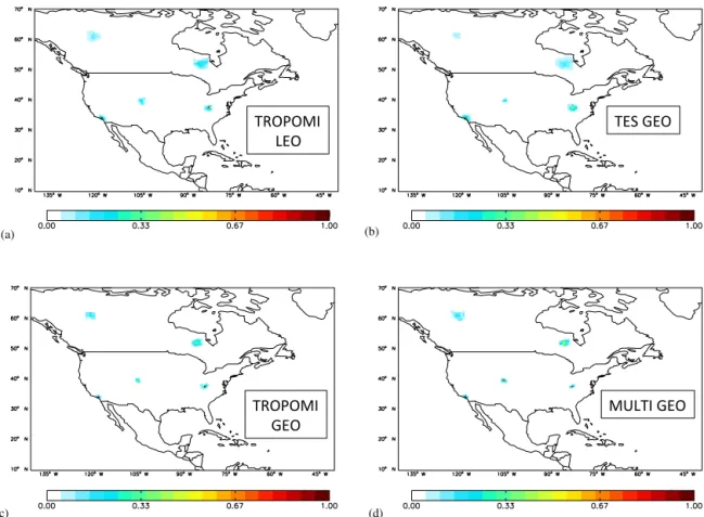
3.2 Spatial resolution of the inversion

An objective measure of the spatial resolution of the inver-sion, i.e., the ability of the observational system to constrain grid-scale emissions independently of each other, is provided by the rows of the model resolution matrix (see Eq. 5). Fig-ure 8 shows the model resolution matrix rows of the weekly inversion corresponding to five different locations, chosen to span a range of characteristics, in terms of emissions mag-nitude and error reduction. For readability, only grid cells included within the largest circle centered on each location

and containing values greater than 0.05 are shown. Table 1 summarizes the coordinates and CH4emissions

(9)

(a) (b)

(c) (d)

DOFs=266

DOFs=115 DOFs=38

DOFs=397

TROPOMI

LEO

TES GEO

TROPOMI

GEO

MULTI GEO

constrained flux patterns is about 2 times higher in the case of a GEO configuration (radius∼80 km) compared to a LEO configuration (radius ∼160 km). Based on the comparison between the TROPOMI_GEO and MULTI_GEO configura-tions, the gain in spatial resolution afforded by the use of a multi-spectral instrument appears significant (factor of 2) only over the eastern US region. Note that although the sizes of the flux structures are similar between the TES_GEO and TROPOMI_LEO configurations, the average values of the model resolution matrix row within each structure are sig-nificantly higher in the case of TROPOMI_LEO.

3.3 Impact of boundary and initial conditions uncertainties

Boundary and initial conditions used in the forward trans-port model contain errors. Therefore, any consistent flux in-version system should jointly optimize the fluxes, initial state and boundary conditions. However, in practice, many studies overlook this issue and optimize those quantities separately (e.g., Basu et al., 2013; Deng et al., 2014). In the latter case, a flux-only inversion is performed with initial and boundary

conditions that are effectively assumed perfectly known. It is therefore of interest to estimate the impact of errors in the initial and boundary conditions on the optimized fluxes. Fig-ure 9 shows the perturbations in the optimized emission scal-ing factors for the weekly inversion resultscal-ing from random Gaussian perturbations of the boundary conditions with stan-dard deviation 16 ppb. The choice for the stanstan-dard error of the noise is based on model–data comparisons from the HIA-PER Pole-to-Pole Observations (HIPPO) experiment (Turner et al., 2015), which consists in extensive aircraft measure-ments throughout the troposphere over the Pacific Ocean. Only weekly inversion results are shown here, so that enough constraints are obtained for all observational configurations while keeping the computational cost of the inversions man-ageable.

(10)

Table 2.Coordinates of the five locations considered for the rows of the model resolution matrix and approximate radius of influence of neighboring grid cells (see text), for each satellite configuration and a weekly methane flux inversion.

Region Coordinates TES_GEO TROPOMI_LEO TROPOMI_GEO MULTI_GEO (lon, lat (◦)) Radius (km) Radius (km) Radius (km) Radius (km)

Eastern US (−82, 38) 160 160 160 80

Central US (−104, 40) 79 158 79 79

California (−117.3, 34.5) 164 164 82 82

Western Canadian wetlands (−120, 61.5) 130 196 131 196

Eastern Canadian wetlands (−84.6, 52.5) 283 213 142 142

TES GEO

TROPOMI LEO

TROPOMI GEO

MULTI GEO

(a)

(b)

(c)

Figure 7.Relative error variance reduction as a function of methane emission magnitude for a(a)30-day (1–30 July 2008),(b)7-day (1–8 July 2008), and(c) 3-day (1–4 July 2008) inversion. Blue: TROPOMI low-Earth orbit observations (TROPOMI_LEO); green: GEO-CAPE observations with a TES-like instrument (TES_GEO); red: GEO-CAPE observations with a TROPOMI-like instru-ment (TROPOMI_GEO); black: GEO-CAPE observations with a multi-spectral instrument (MULTI_GEO). Results for a 3-day MULTI_GEO inversion are also shown in purple (top). The verti-cal bars indicate the standard deviation of observational constraints within each bin.

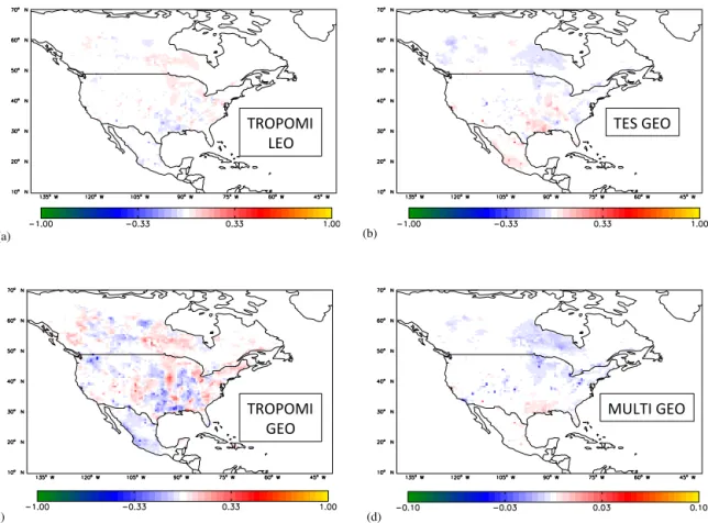
the optimized scaling factors to boundary conditions, with large areas characterized by perturbations between 10 and 50 %, and with impacts greater than 50 % locally. In com-parison, the TROPOMI_GEO configuration shows smaller

sensitivities to boundary conditions, with perturbations gen-erally smaller than 30 %. The MULTI_GEO results are in contrast to the other configurations, with most scaling factor perturbations being smaller than 5 %.

The differences between the sensitivities of the optimized fluxes to boundary conditions for different observational sys-tems are driven by two factors: (1) the sensitivity of the ob-servations to the underlying fluxes (defined by the opera-torH) and (2) the model–data mismatch (i.e.,H (x)−y)). This can be seen, e.g., by considering the observational term in the gradient formula of Eq. (2). Formally, a per-turbation of the boundary conditions will translate into a corresponding perturbation of the observations (y) in the model–data mismatch, which is propagated into flux scal-ing factor perturbations through the adjoint matrix of sen-sitivities (HT). The effect of (1) is clearly seen when com-paring the TROPOMI_GEO and TROPOMI_LEO results, the higher temporal frequency of the geostationary obser-vations providing higher sensitivity to the fluxes. The effect of (2) is best illustrated by comparing the TROPOMI_GEO and MULTI_GEO results. Indeed, since the multi-spectral measurements allow for distinguishing boundary layer from free tropospheric CH4 concentrations, and given the

uni-form (∼1) sensitivity of the TROPOMI column measure-ments throughout the troposphere (see Fig. 2), the boundary layer model–data mismatch (MULTI_GEO) is much smaller than the column model–data mismatch (TROPOMI_GEO), which results in much higher flux adjustments for the TROPOMI_GEO configuration.

The same analysis applies to the sensitivities of the op-timized fluxes to initial conditions, which are shown in Fig. 10. Here the CH43-D initial concentrations were

(11)

(a) (b)

(c) (d)

TROPOMI

LEO

TES GEO

TROPOMI

GEO

MULTI GEO

Figure 8.Rows of the model resolution matrix (unitless) for five locations for a 7-day inversion (1–8 July 2008), using(a)TROPOMI low-Earth orbit observations (TROPOMI_LEO); (b)GEO-CAPE observations with a TES-like instrument (TES_GEO);(c)GEO-CAPE observations with a TROPOMI-like instrument (TROPOMI_GEO); and (d) GEO-CAPE observations with a multi-spectral instrument (MULTI_GEO). Coordinates of the five locations considered are reported in Table 1 and approximately correspond to the peak value of each structure on the maps.

significant sensitivities to CH4concentrations throughout the

troposphere with high-frequency measurements, is most sen-sitive to initial condition perturbations, with up to 30 % vari-ability in the optimized scaling factors. The TROPOMI_LEO and TES_GEO configurations show comparable sensitivities, with scaling factor perturbations generally smaller than 10 %. Similarly to the boundary condition case, initial condition sensitivities associated with the MULTI_GEO configuration are about 1 order of magnitude smaller than other configu-rations, with scaling factor perturbations generally smaller than 3 %. These results show that although the advantage of a multi-spectral instrument in terms of spatiotemporal con-straints on the fluxes becomes significant only for timescales smaller than a week, there is still a clear benefit in using this configuration to mitigate the impact of uncertainties in boundary and initial conditions on the inversion, even when optimizing fluxes at coarser temporal resolution (e.g., weekly or monthly).

4 Conclusions

In this paper we evaluated top-down constraints on methane emissions in North America provided by future potential geostationary (GEO-CAPE) and planned low-Earth orbit (TROPOMI) remote-sensing observation missions. For the first time, a grid-scale estimate of the information content of a high resolution inversion (0.5◦×0.7◦over North America) in a 4D-Var inversion framework has been performed using an efficient stochastic algorithm. In particular, this allowed us to compute both the relative error reductions and the spa-tial correlations between observational constraints in the in-version. Instrument configurations corresponding to TIR and SWIR methane retrievals (TES-like and TROPOMI, respec-tively), as well as a potential future multi-spectral retrieval, were considered. This allowed us to assess the relative im-portance of the vertical sensitivity of the measurement versus the spatiotemporal resolution of the sampling (GEO versus LEO) in methane flux inversions.

(12)

(a) (b)

(c) (d)

TROPOMI

LEO

TES GEO

TROPOMI

GEO

MULTI GEO

Figure 9.Sensitivity of the optimized emission scaling factors to uncertainties in boundary conditions for a 7-day inversion (1–8 July 2008), using(a)TROPOMI low-Earth orbit observations (TROPOMI_LEO);(b)GEO-CAPE observations with a TES-like instrument (TES_GEO); (c)GEO-CAPE observations with a TROPOMI-like instrument (TROPOMI_GEO); and(d)GEO-CAPE observations with a multi-spectral instrument (MULTI_GEO). Shown is the impact of perturbations of the boundary condition concentrations with Gaussian distribution N(0.16 ppb) on the optimized scaling factors. Note the different color scale for the MULTI_GEO configuration.

of error reductions in the optimized fluxes when the targeted timescales are about a week or less. For a 3-day inversion, the number of pieces of information (DOF) independently constrained by the GEO observations is about twice as many as in the case of a LEO configuration (DOF of 266 and 115, respectively). Experiments with TIR GEO and SWIR LEO configurations demonstrated that the high temporal fre-quency of GEO observations cannot compensate for weak sensitivities of the satellite measurement to boundary layer concentrations, since constraints from a TES-like instrument in GEO orbit correspond to only about half of the information content afforded by a TROPOMI instrument in LEO orbit for a monthly inversion (DOF of 164 and 298, respectively). In a GEO orbit, the benefit of using a multi-spectral instru-ment compared to a SWIR instruinstru-ment has been demonstrated for weekly to sub-weekly scale flux constraints, with an in-crease in the DOF of about 50 % for a 3-day inversion. For the multi-spectral GEO configuration, the information con-tent is similar for a 3-day or a 1-month optimization (DOF of 397 and 398, respectively). Moreover, comparison of our re-sults with those from a recent CH4inversion study by Turner

et al. (2015) suggests that TROPOMI or GEO-CAPE could improve monthly-scale constraints on emissions by about an order of magnitude relative to GOSAT.

Over some local CH4 source hotspots (emissions

>4×105kg day−1) in the central US, California and east-ern US, both SWIR and multi-spectral GEO configurations allow for nearly complete constraints on emissions (error re-duction close to 100 %) at a spatial resolution smaller than 100 km×100 km. These estimates are optimistic, given the lack of spatial error correlation considered in our prior emis-sions, which should be addressed in future work, but do re-veal the potential spatial resolution provided by the measure-ments alone.

(13)

(a) (b)

(c) (d)

TROPOMI

LEO

TES GEO

TROPOMI

GEO

MULTI GEO

Figure 10.Sensitivity of the optimized emission scaling factors to uncertainties in initial condition concentrations for a 7-day inversion (1– 8 July 2008), using(a)TROPOMI low-Earth orbit observations (TROPOMI_LEO);(b)GEO-CAPE observations with a TES-like instrument (TES_GEO);(c)GEO-CAPE observations with a TROPOMI-like instrument (TROPOMI_GEO); and(d)GEO-CAPE observations with a multi-spectral instrument (MULTI_GEO). Shown is the impact on the optimized emission scaling factors of perturbations of the boundary layer and free troposphere initial CH₄ concentrations with Gaussian distributionsN(0.22 ppb) andN(0.46 ppb), respectively. Note the different color scale for the MULTI_GEO configuration.

With growing concerns about the environmental impacts of CH4emissions from the oil and gas industry and the urge

for better monitoring of the US’ CH4budget, a multi-spectral

instrument onboard geostationary orbit would provide a key tool to characterize the variability of the CH4 fluxes at a

weekly to sub-weekly timescale, while greatly mitigating the impact of inverse method uncertainties on the optimized fluxes. Moreover, such an observational system would allow for better understanding of the critical role of wetlands in the global methane budget and their impact on climate change (e.g., Bloom et al., 2012; Miller et al., 2014). Further in-vestigations would be needed to quantify the sensitivity of these results to the choice of the reference CH4emission

in-ventory, since significant discrepancies in the magnitude and spatiotemporal distributions of CH4 sources exist between

current bottom-up inventories (Kirschke et al., 2013). In our study we have neglected prior error correlations in the absence of robust data and methodology to rigorously es-timate them. Since error correlations in prior bottom-up in-ventories nevertheless exist, additional experiments should be performed to test the sensitivity of our information

(14)

Acknowledgements. This project was supported by NASA GEO-CAPE Science Team grant NNX14AH02G and NOAA grant NA14OAR4310136. This work utilized the Janus supercomputer, which is supported by the National Science Foundation (award number CNS-0 821 794) and the University of Colorado Boulder. The Janus supercomputer is a joint effort of the University of Colorado Boulder, the University of Colorado Denver and the National Center for Atmospheric Research. Alexander J. Turner was supported by a Department of Energy (DOE) Computational Science Graduate Fellowship (CSGF). Part of this research was carried out at the Jet Propulsion Laboratory, California Institute of Technology, under a contract with the National Aeronautics and Space Administration.

Edited by: M. Palm

References

Basu, S., Guerlet, S., Butz, A., Houweling, S., Hasekamp, O., Aben, I., Krummel, P., Steele, P., Langenfelds, R., Torn, M., Bi-raud, S., Stephens, B., Andrews, A., and Worthy, D.: Global CO2

fluxes estimated from GOSAT retrievals of total column CO₂, Atmos. Chem. Phys., 13, 8695–8717, doi:10.5194/acp-13-8695-2013, 2013.

Bloom, A. A., Palmer, P. I., Fraser, A., and Reay, D. S.: Sea-sonal variability of tropical wetland CH4emissions: the role of

the methanogen-available carbon pool, Biogeosciences, 9, 2821– 2830, doi:10.5194/bg-9-2821-2012, 2012.

Bocquet, M., Wu, L., and Chevallier, F.: Bayesian design of control space for optimal assimilation of observations. Part I: Consistent multiscale formalism, Q. J. Roy. Meteor. Soc., 137, 1340–1356, doi:10.1002/qj.837, 2011.

Bousserez, N., Henze, D. K., Perkins, A., Bowman, K. W., Lee, M., Liu, J., Deng, F., and Jones, D. B. A.: Improved analysis-error covariance matrix for high-dimensional variational inver-sions: application to source estimation using a 3-D atmospheric transport model, Q. J. Roy. Meteor. Soc., 141, 1906–1921, doi:10.1002/qj.2495, 2015.

Butz, A., Hasekamp, O. P., Frankenberg, C., Vidot, J., and Aben, I.: CH₄retrievals from space-based solar backscatter mea-surements: Performance evaluation against simulated aerosol and cirrus loaded scenes, J. Geophys. Res., 115, D24302, doi:10.1029/2010JD014514, 2010.

Caulton, D. R., Shepson, P. B., Santoro, R. L., Sparks, J. P., Howarth, R. W., Ingraffea, A. R., Cambaliza, M. O., Sweeney, C., Karion, A., Davis, K. J., Stirm, B. H., Montzka, S. A., and Miller, B. R.: Toward a better understanding and quantification of methane emissions from shale gas development, P. Natl. Acad. Sci. USA, 111, 6237–6242, 2014.

Chance, K., Liu, X., Suleiman, R. M., Flittner, D. E., Al-Saadi, J., and Janz, S. J.: Tropospheric emissions: monitoring of pollution (TEMPO), Proc. SPIE 8866, Earth Observing Systems XVIII, 88660D (23 September 2013), doi:10.1117/12.2024479, 2013. Chevallier, F., Bréon, F. M., and Rayner, P. J.: Contribution of the

Orbiting Carbon Observatory to the estimation of CO2sources

and sinks: Theoretical study in a variational data assimilation framework, J. Geophys. Res.-Atmos., 112, 2156–2202, 2007.

Connor, B. J., Boesch, H., Toon, G., Sen, B., Miller, C., and Crisp, D.: Orbiting Carbon Observatory: Inverse method and prospective error analysis, J. Geophys. Res.-Atmos., 113, D05305, doi:10.1029/2006JD008336, 2008.

Cressot, C., Chevallier, F., Bousquet, P., Crevoisier, C., Dlu-gokencky, E. J., A., Fortems-Cheiney, A., Frankenberg, C., Parker, R., Pison, I., Scheepmaker, R. A., Montzka, S. A., Montzka, S. A., Krummel, P. B., Steele, L. P., and Langen-felds, R. L.: On the consistency between global and regional methane emissions inferred from SCIAMACHY, TANSO-FTS, IASI and surface measurements, Atmos. Chem. Phys., 14, 577– 592, doi:10.5194/acp-14-577-2014, 2014.

Deng, F., Jones, D. B. A., Henze, D. K., Bousserez, N., Bowman, K. W., Fisher, J. B., Nassar, R., O’Dell, C., Wunch, D., Wennberg, P. O., Kort, E. A., Wofsy, S. C., Blumenstock, T., Deutscher, N. M., Griffith, D. W. T., Hase, F., Heikkinen, P., Sherlock, V., Strong, K., Sussmann, R., and Warneke, T.: Inferring regional sources and sinks of atmospheric CO2from GOSAT XCO2data,

Atmos. Chem. Phys., 14, 3703–3727, doi:10.5194/acp-14-3703-2014, 2014.

Dlugokencky, E. J., Nisbet, E. G., Fisher, R., and Lowry, D.: Global atmospheric methane: budget, changes and dangers, Philos. T. R. Soc. A, 369, 2058–2072, 2011.

European Commission: Emission Database for Global Atmospheric Research (EDGAR), release version 4.2, Tech. rep., Joint Re-search Centre (JRC)/Netherlands Environmental Assessment Agency (PBL), available at: http://edgar.jrc.ec.europa.eu (last ac-cess: 1 December 2014), 2011.

Fiore, A. M., Jacob, D. J., Field, B. D., Streets, D. G., Fernan-des, S. D., and Jang, C.: Linking ozone pollution and climate change: the case for controlling methane, Geophys. Res. Lett., 29, 25–1, 2002.

Fiore, A. M., West, J. J., Horowitz, L. W., Naik, V., and Schwarzkopf, M. D.: Characterizing the tropospheric ozone re-sponse to methane emission controls and the benefits to climate and air quality, J. Geophys. Res.-Atmos., 113, 1984–2012, 2008. Fishman, J., Iraci, L., Al-Saadi, J., Chance, K., Chavez, F., Chin, M., Coble, P., Davis, C., DiGiacomo, P., Edwards, D., Eldering, L., Goes, J., Herman, J., Hu, C., Jacob, D. J., Jordan, C., Kawa, S. R., Key, R., Liu, X., Lohrenz, S., Mannino, A., Natraj, V., Neil, D., Neu, J., Newchruch, M., Pickering, K., Salisbury, J., Sosik, H., Subramaniam, A., Tzortziou, M., Wang, J., and Wang, M.: The United States’ next generation of atmospheric composition and coastal ecosystem measurements: NASA’s Geostationary Coastal and Air Pollution Events (GEO-CAPE) Mission, B. Am. Meteo-rol. Soc., 93, 1547–1566, 2012.

Fu, D., Worden, J. R., Liu, X., Kulawik, S. S., Bowman, K. W., and Natraj, V.: Characterization of ozone profiles derived from Aura TES and OMI radiances, Atmos. Chem. Phys., 13, 3445–3462, doi:10.5194/acp-13-3445-2013, 2013.

Fung, I., John, J., Lerner, J., Matthews, E., Prather, M., Steele, L., and Fraser, P.: Three-dimensional model synthesis of the global methane cycle, J. Geophys. Res.-Atmos., 96, 13033–13065, 1991.

Gazovic, M., Kutzbach, L., Schreiber, P., Wille, C., and Wilmk-ing, M.: Diurnal dynamics of CH4from a boreal peatland during

(15)

Kaplan, J. O.: Wetlands at the Last Glacial Maximum: distribu-tion and methane emissions, Geophys. Res. Lett., 29, 3-1–3-4, doi:10.1029/2001GL013366, 2002.

Karion, A., Sweeney, C., Pétron, G., Frost, G., Michael Hard-esty, R., Kofler, J., Miller, B. R., Newberger, T., Wolter, S., Banta, R., Brewer, A., Dlugokencky, E., Lang, P., Montzka, S. A., Schnell, R., Tans, P., Trainer, M., Zamora, R., and Conley, S.: Methane emissions estimate from airborne measurements over a western United States natural gas field, Geophys. Res. Lett., 40, 4393–4397, 2013.

Katzenstein, A. S., Doezema, L. A., Simpson, I. J., Blake, D. R., and Rowland, F. S.: Extensive regional atmospheric hydrocarbon pollution in the southwestern United States, P. Natl. Acad. Sci. USA, 100, 11975–11979, 2003.

Kirschke, S., Bousquet, P., Ciais, P., Saunois, M., Canadell, J. G., Dlugokencky, E. J., Bergamaschi, P., Bergmann, D., Blake, D. P., Bruhwiler, L., Cameron-Smith, P., Castaldi, P., Chevallier, F., Feng, L., Fraser, A., Heimann, M., Hodson, E. L., Houweling, S., Josse, B., Fraser, P. J., Krummel, P. B., Lamarque, J. F., Langen-felds, R. L., Le Quere, C., Naik, V., O’Doherty, S., Palmer, P. I., Pison, I., Plummer, D., Poulter, B., Prinn, R. G., Rigby, M., Ringeval, B., Santini, M., Schmidt, M., Shindell, D. T., Simp-son, I. J., Spahni, R., Steele, L. P., Strode, S. A., Sudo, K., Szopa, S., van der Werf, G. R., Voulgarakis, A., van Weele, M., Weiss, R. F., Williams, J. E., and Zen, G.: Three decades of global methane sources and sinks, Nat. Geosci., 6, 813–823, 2013. Kort, E. A., Eluszkiewicz, J., Stephens, B. B., Miller, J. B.,

Ger-big, C., Nehrkorn, T., Daube, B. C., Kaplan, J. O., Houweling, S., and Wofsy, S. C.: Emissions of CH4and N2O over the United

States and Canada based on a receptor-oriented modeling frame-work and COBRA-NA atmospheric observations, Geophys. Res. Lett., 35, L18808, doi:10.1029/2008GL034031, 2008.

Kulawik, S. S., Worden, J., Eldering, A., Bowman, K., Gunson, M., Osterman, G. B., Zhang, L., Clough, S., Shephard, M. W., and Beer, R.: Implementation of cloud retrievals for Tropospheric Emission Spectrometer (TES) atmospheric retrievals: part 1. De-scription and characterization of errors on trace gas retrievals, J. Geophys. Res., 111, D24204, doi:10.1029/2005JD006733, 2006. Lions, J. L.: Optimal Control of Systems Governed by Partial

Dif-ferential Equations, Springer-Verlag, Berlin, 1971.

Liu, J., Bowman, K., Lee, M., Henze, D. K., Bousserez, N., Brix, H., Collatz, G., Menemenlis, D., Ott, L., Pawson, S., Jones, D., and Nassar, R.: Carbon monitoring system flux estimation and at-tribution: impact of ACOS-GOSAT XCO2sampling on the

in-ference of terrestrial biospheric sources and sinks, Tellus B, 66, 22486, doi:10.3402/tellusb.v66.22486, 2014.

Locatelli, R., Bousquet, P., Chevallier, F., Fortems-Cheney, A., Szopa, S., Saunois, M., Agusti-Panareda, A., Bergmann, D., Bian, H., Cameron-Smith, P., Chipperfield, M. P., Gloor, E., Houweling, S., Kawa, S. R., Krol, M., Patra, P. K., Prinn, R. G., Rigby, M., Saito, R., and Wilson, C.: Impact of transport model errors on the global and regional methane emissions estimated by inverse modelling, Atmos. Chem. Phys., 13, 9917–9937, doi:10.5194/acp-13-9917-2013, 2013.

Meirink, J. F., Bergamaschi, P., and Krol, M. C.: Four-dimensional variational data assimilation for inverse modelling of atmospheric methane emissions: method and comparison with synthesis inversion, Atmos. Chem. Phys., 8, 6341–6353, doi:10.5194/acp-8-6341-2008, 2008.

Miller, S. M., Wofsy, S. C., Michalak, A. M., Kort, E. A., An-drews, A. E., Biraud, S. C., Dlugokencky, E. J., Eluszkiewicz, J., Fischer, M. L., Janssens-Maenhout, G., Miller, B. R., Miller, J. B., Montzkad, S. A., Nehrkornf, T., and Sweene, C.: Anthropogenic emissions of methane in the United States, P. Natl. Acad. Sci. USA, 110, 20018–20022, 2013.

Miller, S. M., Worthy, D. E., Michalak, A. M., Wofsy, S. C., Kort, E. A., Havice, T. C., Andrews, A. E., Dlugokencky, E. J., Kaplan, J. O., Levi, P. J., Tian, H., and Zhang, B.: Observational constraints on the distribution, seasonality, and environmental predictors of North American boreal methane emissions, Global Biogeochem. Cy., 28, 146–160, 2014.

Morin, T. H., Bohrer, G., Naor-Azrieli, L., Mesi, S., Kenny, W. T., Mitsch, W. J., and Schaefer, K. V. R.: The seasonal and diurnal dynamics of methane flux at a created urban wetland, Ecol. Eng., 72, 74–83, 2014.

Myhre, G. and Shindell, D.: Climate Change 2013: The Physi-cal Science Basis, Intergovernmental Panel on Climate Change (IPCC), Chap. 8, Cambridge University Press, 2013.

Parker, R., Boesch, H., Cogan, A., Fraser, A., Feng, L., Palmer, P. I., Messerschmidt, J., Deutscher, N., Griffith, D. W., Notholt, J., Wennberg, P. O., and Wunch, D.: Methane observations from the Greenhouse Gases Observing SATellite: comparisonn to ground-based TCCON data and model calculations, Geophys. Res. Lett., 38, L15807, doi:10.1029/2011GL047871, 2011.

Pickett-Heaps, C. A., Jacob, D. J., Wecht, K. J., Kort, E. A., Wofsy, S. C., Diskin, G. S., Worthy, D. E. J., Kaplan, J. O., Bey, I., and Drevet, J.: Magnitude and seasonality of wetland methane emissions from the Hudson Bay Lowlands (Canada), Atmos. Chem. Phys., 11, 3773–3779, doi:10.5194/acp-11-3773-2011, 2011.

Polonsky, I. N., O’Brien, D. M., Kumer, J. B., O’Dell, C. W., and the geoCARB Team: Performance of a geostationary mission, geoCARB, to measure CO2, CH4and CO column-averaged

con-centrations, Atmos. Meas. Tech., 7, 959–981, doi:10.5194/amt-7-959-2014, 2014.

Rayner, P. J., Utembe, S. R., and Crowell, S.: Constraining re-gional greenhouse gas emissions using geostationary concentra-tion measurements: a theoretical study, Atmos. Meas. Tech., 7, 3285–3293, doi:10.5194/amt-7-3285-2014, 2014.

Shindell, D., Kuylenstierna, J. C., Vignati, E., van Dingenen, R., Amann, M., Klimont, Z., Anenberg, S. C., Muller, N., Janssens-Maenhout, G., Raes, F., Schwartz, J., Faluvegi, G., Pozzoli, L., Kupiainen, K., Hoglund-Isaksson, L., Emberson, L., Streets, D., Ramanathan, V., Hicks, K., Oanh, N., Milly, G., Williams, M., Demkine, V., and Fowler, D.: Simultaneously mitigating near-term climate change and improving human health and food secu-rity, Science, 335, 183–189, 2012.

Tarantola, A.: Inverse problem theory and methods for model parameter estimation, SIAM, doi:10.1137/1.9780898717921, 2005.

Turner, A. J. and Jacob, D. J.: Balancing aggregation and smoothing errors in inverse models, Atmos. Chem. Phys., 15, 7039–7048, doi:10.5194/acp-15-7039-2015, 2015.

(16)

Wennberg, P. O., and Wunch, D.: Estimating global and North American methane emissions with high spatial resolution us-ing GOSAT satellite data, Atmos. Chem. Phys., 15, 7049–7069, doi:10.5194/acp-15-7049-2015, 2015.

van der Werf, G. R., Randerson, J. T., Giglio, L., Collatz, G. J., Mu, M., Kasibhatla, P. S., Morton, D. C., DeFries, R. S., Jin, Y., and van Leeuwen, T. T.: Global fire emissions and the contribution of deforestation, savanna, forest, agricultural, and peat fires (1997–2009), Atmos. Chem. Phys., 10, 11707–11735, doi:10.5194/acp-10-11707-2010, 2010.

Wecht, K. J., Jacob, D. J., Wofsy, S. C., Kort, E. A., Worden, J. R., Kulawik, S. S., Henze, D. K., Kopacz, M., and Payne, V. H.: Val-idation of TES methane with HIPPO aircraft observations: impli-cations for inverse modeling of methane sources, Atmos. Chem. Phys., 12, 1823–1832, doi:10.5194/acp-12-1823-2012, 2012. Wecht, K. J., Jacob, D. J., Frankenberg, C., Jiang, Z., and

Blake, D. R.: Mapping of North American methane emissions with high spatial resolution by inversion of SCIAMACHY satel-lite data, J. Geophys. Res.-Atmos., 119, 7741–7756, 2014a. Wecht, K. J., Jacob, D. J., Sulprizio, M. P., Santoni, G. W.,

Wofsy, S. C., Parker, R., Bösch, H., and Worden, J.: Spatially resolving methane emissions in California: constraints from the CalNex aircraft campaign and from present (GOSAT, TES) and future (TROPOMI, geostationary) satellite observations, Atmos. Chem. Phys., 14, 8173–8184, doi:10.5194/acp-14-8173-2014, 2014b.

West, J. J. and Fiore, A. M.: Management of tropospheric ozone by reducing methane emissions, Environ. Sci. Technol., 39, 4685– 4691, 2005.

West, J. J., Fiore, A. M., Horowitz, L. W., and Mauzerall, D. L.: Global health benefits of mitigating ozone pollution with methane emission controls, P. Natl. Acad. Sci. USA, 103, 3988– 3993, 2006.

West, J. J., Fiore, A. M., and Horowitz, L. W.: Scenarios of methane emission reductions to 2030: abatement costs and co-benefits to ozone air quality and human mortality, Climatic Change, 114, 441–461, 2012.

Worden, J., Kulawik, S., Shephard, M. W., Clough, S. A., Wor-den, H., Bowman, K., and Goldman, A.: Predicted errors of tropospheric emission spectrometer nadir retrievals from spectral window selection, J. Geophys. Res., 109, D09308, doi:10.1029/2004JD004522, 2004.

Worden, J., Kulawik, S., Frankenberg, C., Payne, V., Bowman, K., Cady-Peirara, K., Wecht, K., Lee, J.-E., and Noone, D.: Pro-files of CH4, HDO, H2O, and N2O with improved lower

tro-pospheric vertical resolution from Aura TES radiances, Atmos. Meas. Tech., 5, 397–411, doi:10.5194/amt-5-397-2012, 2012. Worden, J. R., Turner, A. J., Bloom, A., Kulawik, S. S., Liu, J.,

Lee, M., Weidner, R., Bowman, K., Frankenberg, C., Parker, R., Payne, V. H.: Quantifying lower tropospheric methane concen-trations using GOSAT near-IR and TES thermal IR measure-ments, Atmos. Meas. Tech., 8, 3433–3445, doi:10.5194/amt-8-3433-2015, 2015.

Xiao, Y., Logan, J. A., Jacob, D. J., Hudman, R. C., Yantosca, R., and Blake, D. R.: Global budget of ethane and regional con-straints on US sources, J. Geophys. Res.-Atmos., 113, D21306, doi:10.1029/2007JD009415, 2008.

Yevich, R. and Logan, J. A.: An assessment of biofuel use and burn-ing of agricultural waste in the developburn-ing world, Global Bio-geochem. Cy., 17, 1095, doi:10.1029/2002GB001952, 2003. Zhu, L., Henze, D., Bash, J. O., Cady-Pereira, K. E.,

Shep-hard, M. W., Luo, M., and Capps, S. L.: Sources and impacts of atmospheric NH3: Current understanding and frontiers for