www.atmos-chem-phys.net/15/305/2015/ doi:10.5194/acp-15-305-2015
© Author(s) 2015. CC Attribution 3.0 License.
Simulations of atmospheric methane for Cape Grim, Tasmania,
to constrain southeastern Australian methane emissions
Z. M. Loh1, R. M. Law1, K. D. Haynes1,*, P. B. Krummel1, L. P. Steele1, P. J. Fraser1, S. D. Chambers2, and A. G. Williams2
1Centre for Australian Weather and Climate Research, CSIRO Oceans and Atmosphere Flagship,
Private Bag 1, Aspendale, Vic 3195, Australia
2Australian Nuclear Science and Technology Organisation, Locked Bag 2001, Kirrawee DC, NSW 2232, Australia *now at: Department of Atmospheric Science, Colorado State University, Fort Collins, CO, USA
Correspondence to:R. M. Law ([email protected])
Received: 1 August 2014 – Published in Atmos. Chem. Phys. Discuss.: 19 August 2014 Revised: 26 November 2014 – Accepted: 17 December 2014 – Published: 13 January 2015
Abstract. This study uses two climate models and six sce-narios of prescribed methane emissions to compare modelled and observed atmospheric methane between 1994 and 2007, for Cape Grim, Australia (40.7◦S, 144.7◦E). The model simulations follow the TransCom-CH4protocol and use the
Australian Community Climate and Earth System Simulator (ACCESS) and the CSIRO Conformal-Cubic Atmospheric Model (CCAM). Radon is also simulated and used to re-duce the impact of transport differences between the mod-els and observations. Comparisons are made for air samples that have traversed the Australian continent. All six emis-sion scenarios give modelled concentrations that are broadly consistent with those observed. There are three notable mis-matches, however. Firstly, scenarios that incorporate interan-nually varying biomass burning emissions produce anoma-lously high methane concentrations at Cape Grim at times of large fire events in southeastern Australia, most likely due to the fire methane emissions being unrealistically in-put into the lowest model level. Secondly, scenarios with wetland methane emissions in the austral winter overesti-mate methane concentrations at Cape Grim during winter-time while scenarios without winter wetland emissions per-form better. Finally, all scenarios fail to represent a methane source in austral spring implied by the observations. It is pos-sible that the timing of wetland emissions in the scenarios is incorrect with recent satellite measurements suggesting an austral spring (September–October–November), rather than winter, maximum for wetland emissions.
1 Introduction
Methane (CH4) is an important greenhouse gas whose
at-mospheric concentration has more than doubled since the 18th century (MacFarling Meure et al., 2006), with con-siderable variations in its growth rate over recent decades (Rigby et al., 2008; Dlugokencky et al., 2009; Sussmann et al., 2012). Methane has both anthropogenic and natural emissions, while the main sink for methane is through reac-tion with hydroxyl radical (OH) in the troposphere and by photolysis in the stratosphere. On a global scale, consider-able uncertainty remains about the causes of recent changes in the methane growth rate (Kirschke et al., 2013), and on a regional level, significant discrepancies have been found between “bottom up” inventory estimates of emissions and “top down” atmospheric inverse modelling studies. For ex-ample, in Miller et al. (2013), the authors find that the in-ventories underestimate emissions by up to 2.7 times in the south-central USA.
methane and CSIRO flask methane data, together with the AGAGE methyl chloroform records to deduce the Northern Hemisphere and Southern Hemisphere changes in methane emissions required to account for the measured increase in methane mole fraction growth rate from 2007.
Recently a model intercomparison, “TransCom-CH4”, has
been run for methane (Patra et al., 2011), with a focus on understanding how transport model differences contributed to variations in the methane simulations. All model sim-ulations used the same prescribed methane emissions and modelled methane loss using prescribed, climatological OH fields. We have used the simulations defined for this inter-comparison to compare simulated and measured methane at Cape Grim, with the goal of evaluating the accuracy of the prescribed methane emissions for southeastern Australia. The model intercomparison also simulated radon, sulfur hex-afluoride (SF6) and methyl chloroform (CH3CCl3) as
addi-tional tests for different components of the transport model. Radon (222Rn) is emitted reasonably uniformly in both space and time from land surfaces at much higher rates than from oceans and decays radioactively with a half-life of 3.8 days. Due to its short lifetime, radon is often used as a tracer of re-cent contact with land and to explore vertical mixing through the lower atmosphere (Zahorowski et al., 2004; Williams et al., 2011, 2013; Chambers et al., 2011). Since radon fluxes are usually assumed to be better characterized than fluxes of other trace gases, radon has been used, via tracer ratio meth-ods, to estimate regional carbon dioxide, methane and nitrous oxide or other greenhouse gas fluxes (Schmidt et al., 1996; Wilson et al., 1997; Biraud et al., 2000; Zahorowski et al., 2004; Wada et al., 2013).
An Australian methane budget was described by Wang and Bentley (2002), who used 1997 Cape Grim atmo-spheric methane measurements in an inversion to constrain the methane fluxes from southern Australia. Their study suggested that the methane inventory overestimated south-eastern Australian fluxes. A more recent modelling study by Fraser et al. (2011) ran forward model simulations for 2005–2008 and separated methane into different regional and process-based components, focusing on better parameteriz-ing methane fluxes from seasonal wetlands in tropical Aus-tralia. At Cape Grim, they found their simulated methane was dominated by animal, landfill and ocean fluxes. They also noted that their model reproduced background, baseline methane concentrations at Cape Grim well, but the model was less successful in reproducing concentrations influenced by local emissions. The concentration excursions driven by local emissions are typically large in magnitude and are re-ferred to as “non-baseline” events. These events contain in-formation regarding regional fluxes and are the focus of this study.
To investigate non-baseline events, this study uses both ob-servations at Cape Grim and forward model simulations with prescribed emissions. Sections 2 and 3 describe the observa-tions at Cape Grim and the model simulaobserva-tions, respectively.
136 138 140 142 144 146 148 150 152 154 136 138 140 142 144 146 148 150 152 154
44
42
40
38
36
34
32
44
42
40
38
36
34
32
Longitude (˚E)
Latitude (˚S)
Mainland Australia
Melbourne
Bass Strait
Tasmania
ACCESS CCAM Cape Grim
144 145 146 144 145 146
41
40
39
41
40
39
Cape Grim ACCESS
CCAM
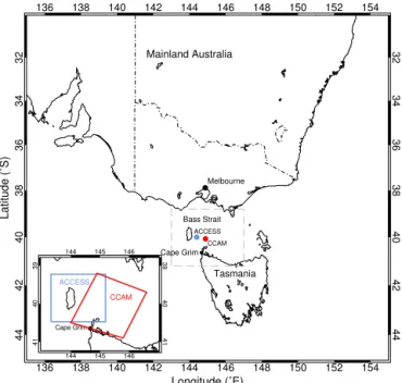
Figure 1.Map of southeastern Australia, showing the location of
the Cape Grim Baseline Air Pollution Station, along with the AC-CESS (blue) and CCAM (red) grid points selected to best represent Cape Grim. The choice of these grid points is discussed in Sect. 4.2. The inset shows the extent of each of the grid cells.
Section 4 focuses on seasonal-scale results, exploring an ap-parent anomaly between modelled and observed methane in austral spring. The implications for regional methane fluxes are discussed in Sect. 5.
2 Observations
Cape Grim is located at the top of a 90 m cliff on the north-west coast of Tasmania (40.7◦S, 144.7◦E), which is sepa-rated from mainland Australia by Bass Strait (Fig. 1). The Cape Grim station has been operating since the 1970s and now has the most comprehensive monitoring programme in the Southern Hemisphere for greenhouse gases (Langenfelds et al., 2014), ozone-depleting gases (Krummel et al., 2014) and radon (Zahorowski et al., 2014).
cy-Jan Feb Mar Apr May Jun Jul Aug Sep Oct Nov Dec Jan
2006 2007
1700 1750 1800 1850 1900
CH
4
(ppb)
(a)
Jan Feb Mar Apr May Jun Jul Aug Sep Oct Nov Dec Jan
2006 2007
0 2 4 6 8 10
Radon (Bq m
-3) (b)
01 02 03 04 05 06 07 08 09 10 11 12 13 14 15 16 17 18 19 20 21 22 23 24 25 26 27 28 29 30 31 January 2006
1700 1720 1740 1760 1780 1800
CH
4
(ppb)
(c)
01 02 03 04 05 06 07 08 09 10 11 12 13 14 15 16 17 18 19 20 21 22 23 24 25 26 27 28 29 30 31 January 2006
0 1 2 3 4 5
Radon (Bq m
-3) (d)
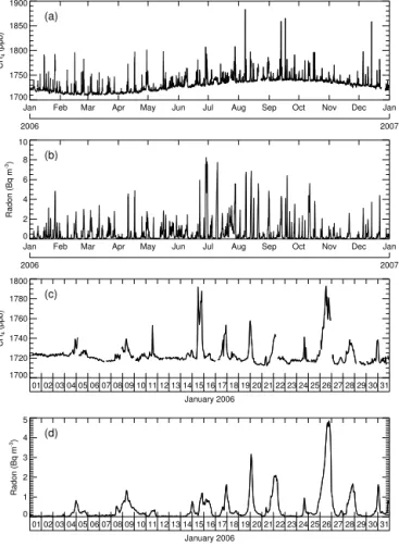
Figure 2.Cape Grim observations(a)2006 methane data(b)2006
radon data (c)January 2006 methane data and(d) January 2006 radon data.
cles in both methane and radon are apparent in Fig. 2a and b which show a full year of data. In Fig. 2c and d, showing just one month of data, the difference between baseline periods and non-baseline events can be more clearly seen and one gets a sense of the degree to which methane and radon are correlated.
Flask measurements of CH4began at Cape Grim in 1984,
while the record from the current AGAGE GC-MD (multi-gas chromatograph, multi-detector) in situ instrument sys-tem, which incorporates a Carle GC fitted with a flame ion-ization detector (see Prinn et al., 2000) began late in 1993. Ambient methane measurements are made on discrete air samples every 40 min, taken alternately from a 75 and 10 m inlet for the majority of the study period. The data from both inlets are used in this study. Ambient samples are bracketed by analysis of a calibration standard, and the resulting CH4
record is reported on the Tohoku University scale (Aoki et al., 1992; Prinn et al., 2000).
During the period of observations used for this study, Cape Grim radon measurements were made using a number of tectors. From 1994 to 1997, a 9000 L two-filter radon de-tector featuring a particle generator was used, operating at
a nominal flow rate of 200 L min−1 and with a response time of approximately 90 min (Whittlestone and Zahorowski, 1995). From 1997, a newly designed 5000 L dual flow loop, two-filter radon detector was commissioned, operating at a nominal flow rate of 285 L min−1and with a response time of 45 min (Whittlestone and Zahorowski, 1998). Later devel-opments saw this new detector enhanced from a single-head design to two and eventually four heads in 2004, with corre-sponding improvements to sensitivity and lower limit of de-tection. Air was sampled from a 75 m inlet, the same height as the upper CH4observations. Raw radon counts were
col-lected half-hourly and aggregated to hourly values during post-processing. Detector sensitivity ranged from 0.6 to 1.2 counts per second per Bq m−3 during the period of mea-surements. Calibrations were performed monthly using a Py-lon flow-through radon source (20.9±0.8 kBq Radium-226),
traceable to US National Institute of Standards and Technol-ogy (NIST) standards, and instrumental background checks were performed approximately every 3 months. The lower limit of detection for the Cape Grim radon detectors, defined as the radon concentration below which the statistical count-ing error exceeds 30 %, ranged from 6 to 10 mBq m−3.
For this study, CH4 observations from 1994–2007 have
been processed using the following steps:
1. We have linearly interpolated between the discrete mea-surements of atmospheric CH4every 40 min, to
gener-ate hourly CH4data, to facilitate comparisons with the
hourly radon data, and the hourly values from the model simulations.
2. The CH4observations were then selected for baseline
conditions by excluding all hours when the coincident radon measurement was greater than 100 mBq m−3.
3. A smooth curve was then found through these baseline-selected CH4 observations using the methodology
de-scribed in Thoning et al. (1989). Specifically, the baseline data are fitted with a function consisting of a second-order polynomial and four harmonics. This function fit is then subtracted from the baseline data and the resulting residuals are then filtered with a band-pass filter with a short-term cut-off of 80 days. The original function fit is then added back to the filtered residuals to give a smooth curve fit through the data. This procedure is performed iteratively, and in each iteration, the indi-vidual hours that lie outside twice the standard deviation around the fit are excluded until the fit converges.
4. Lastly, the smooth curve fitted to the baseline data is subtracted from all CH4observations to give a time
3 Model simulations
This study uses simulation experiments that were run for the TransCom-CH4 model intercomparison to investigate
vari-ous methane flux estimates. The TransCom-CH4 model
in-tercomparison involved running nine tracers in a global at-mospheric model for the years 1988–2007. The first six trac-ers used different methane emission scenarios. The remain-ing three tracers were radon, sulfur hexafluoride and methyl chloroform. In each methane case, chemical loss of methane was simulated using prescribed OH fields (with seasonal variations but no interannual variations) and prescribed loss rates to represent photolysis in the stratosphere. The emis-sions are described in detail and a global analysis of the re-sults is presented in Patra et al. (2011). Other details can also be found online in the TransCom-CH4protocol (Patra et al.,
2010).
3.1 Methane emission scenarios
The six methane scenarios were created by combining var-ious estimates of anthropogenic, rice, biomass burning and wetland components in different ways (Table 1). Details are given in Patra et al. (2011) and we use the same emis-sion scenario labels as used in that paper and across the TransCom-CH4project. The control (CTL) scenario uses
an-thropogenic fluxes as specified in the Emissions Database for Global Atmospheric Research (EDGAR) inventory, ver-sion 3.2 (Olivier and Berdowski, 2001) and includes fossil fuel, industrial, animal, fire, waste and biofuel emissions. Added to these fluxes are seasonally varying (no interannual variability) natural fluxes comprising biomass burning from Fung et al. (1991), wetland emissions (Matthews and Fung, 1987; Fung et al., 1991) and rice (Yan et al., 2009).
Four alternative emissions scenarios change one or more of the CTL component fluxes. CTL_E4 uses EDGAR 4.0 (van Aardenne et al., 2001) for the anthropogenic compo-nent; BB (biomass burning) uses biomass burning emis-sions from the Global Fire Emisemis-sions Database, version 2 (van der Werf et al., 2006) (including interannual variations when available); WLBB (wetland and biomass burning) ad-ditionally includes interannually varying wetland emissions (Ringeval et al., 2010); EXTRA uses the same biomass burn-ing as BB and interannually varyburn-ing model generated wet-lands and rice emissions from the VISIT model (Ito and Inatomi, 2012). A final emissions scenario, INV, does not use fluxes from inventories or process models but those estimated by the atmospheric inversion of Bousquet et al. (2006). All six emissions scenarios use the same soil sink. Table 2 de-tails which components of each scenario include interannual variability and in which years of the simulations.
Figure 3a shows the aggregated emissions for the region of southeastern Australia bounded by 135–155◦E and 45–30◦S which is the region shown in Fig. 1. The emissions show a seasonal cycle that is dominated by the wetland component
J F M A M J J A S O N D
0 2 4 6
Flux (Tg CH
4
yr
-1 )
(a)
1994 1996 1998 2000 2002 2004 2006 2008
0 2 4 6
Flux (Tg CH
4
yr
-1 )
INV
EXTRA WLBB BB CTL_E4 CTL
(b)
Figure 3.Seasonal cycle(a)and annual mean(b)methane fluxes
for 1994–2007 integrated over the SE Australian region (135– 155◦E, 30–45◦S). Six flux scenarios are shown as listed in the key.
for CTL, CTL_E4 and BB with higher emissions from May to October. The seasonality is much smaller for the WLBB and EXTRA scenarios with maximum fluxes in December and January due to biomass burning. The INV emissions show similar seasonality to the CTL emissions, though with smaller amplitude. It is worth noting that the inversion used to generate these fluxes included only baseline CH4 data at
Cape Grim, so there is no reason to expect the INV fluxes to fit the non-baseline record at Cape Grim better than the other flux scenarios.
Figure 3b shows the interannual variability of the pre-scribed emissions, again aggregated over the region shown in Fig. 1. The CTL fluxes show almost no change in time, while the CTL_E4 fluxes increase over time. The three fluxes that include interannually varying biomass burning – BB, WLBB and EXTRA – show peaks in 2003 and 2006 associated with significant summer fires in southeastern Australia. This will be discussed in more detail in Sect. 4.1. The INV fluxes show the greatest interannual variability in this region.
The prescribed TransCom-CH4methane emissions can be
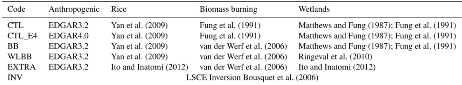
Table 1.The broad components of the methane emission scenarios. The anthropogenic category includes fossil fuel, industrial, animal, fire, waste and biofuel emissions. See Patra et al. (2011) for further details of how the emission scenarios were constructed.
Code Anthropogenic Rice Biomass burning Wetlands
CTL EDGAR3.2 Yan et al. (2009) Fung et al. (1991) Matthews and Fung (1987); Fung et al. (1991) CTL_E4 EDGAR4.0 Yan et al. (2009) Fung et al. (1991) Matthews and Fung (1987); Fung et al. (1991) BB EDGAR3.2 Yan et al. (2009) van der Werf et al. (2006) Matthews and Fung (1987); Fung et al. (1991) WLBB EDGAR3.2 Yan et al. (2009) van der Werf et al. (2006) Ringeval et al. (2010)
EXTRA EDGAR3.2 Ito and Inatomi (2012) van der Werf et al. (2006) Ito and Inatomi (2012)
INV LSCE Inversion Bousquet et al. (2006)
Table 2.Methane emission scenarios, indicating which components have interannual variations over different periods. A mean seasonal cycle
is used outside the listed periods.
Code Anthropogenic Rice Biomass burning Wetlands
CTL 1990:1995:2000 No No No
CTL_E4 1990–2005 No No No
BB As CTL No 1996–2008 No
WLBB As CTL No As BB 1994–2000
EXTRA As CTL 1988–2008 As BB 1988–2008
INV 1988–2005
Table 3.Annual flux emissions (in Tg y−1) from southeastern
Aus-tralia for different years and from different sources.
Source Year Flux
Wang and Bentley (2002) inventory 1997 3.09 Wang and Bentley (2002) inversion 1997 1.93
Fraser et al. (2011) 2008 2.88
This study 1997 2.38–3.82
This study 2008 2.34–4.16
and Fraser et al. (2011) (Table 3). To approximate our re-gion of interest, from Wang and Bentley (2002) we sum their regions A, C and D, which extend slightly further west and north than our region. This gives total anthropogenic emissions (agriculture including cattle, the energy and trans-port sectors and waste management) of 3.39 Tg y−1, using the methodology of the Australian National Greenhouse Gas Inventory (NGGI) coupled with statistical data for 1997 to give a spatially explicit representation of methane emissions. By adding in an estimate of methane uptake by Australian soils, the net anthropogenic flux used in Wang and Bentley (2002) across southeastern Australia is 3.09 Tg y−1. Wang
and Bentley (2002) also adjust their inventory-based estimate by fitting atmospheric CH4 at Cape Grim using an
inver-sion technique. This gives a substantially lower flux estimate (1.93 Tg y−1).
From Fraser et al. (2011) we sum their anthropogenic emissions (agriculture including cattle (and rice, which is very small), the energy sector, waste management and a small amount of prescribed burning) from five regions – New South
Wales, Australian Capital Territory, Victoria, Tasmania and South Australia – to give total anthropogenic emissions of 2.88 Tg y−1 for 2008. Fraser et al. (2011) take emissions
from the EDGAR 3.2 inventory (Olivier et al., 2005), and scale them to the Australian NGGI. Both inventories have total annual CH4emissions which are closer to the annual
emissions of the lower set of methane scenarios used here, but the inventories do not include natural fluxes while the TransCom methane scenarios do. In southeastern Australia, the major natural flux is from wetlands, but the magnitude of this flux is uncertain. The CTL-based emission scenar-ios (CTL, CTL_E4 and BB) include a large 1.24 Tg y−1 component from wetlands for southeastern Australia, taken from Matthews and Fung (1987) and Fung et al. (1991). The WLBB and EXTRA emission scenarios take their estimates of wetland emissions from Ringeval et al. (2010) and Ito and Inatomi (2012), which are close to zero for southeast-ern Australia. Wetland emissions will be discussed further in Sects. 4.2 and 5.
3.2 Atmospheric models
We have run the TransCom-CH4 simulations with two
models: the CSIRO Conformal-Cubic Atmospheric Model (CCAM) (McGregor, 2005; McGregor and Dix, 2008) and the Australian Community Climate and Earth System Simu-lator (ACCESS) (Corbin and Law, 2011). Using two models allows us to better understand any sensitivity in the analysis to model transport error.
horizon-tal resolution of approximately 220 km, and 18 levels in the vertical. The horizontal components of the wind were nudged (Thatcher and McGregor, 2009) to NCEP analyses (Kalnay et al., 1996; Collier, 2004). This helps to ensure that simulated atmospheric concentrations of trace gases can be more realistically compared to observations on synoptic timescales. The CCAM simulations analysed here are the same as those submitted to the TransCom-CH4 experiment
(Patra et al., 2011).
The second model, ACCESS, is derived from the UK Met Office Unified Model but has the land surface scheme re-placed by the Community Atmosphere Biosphere Land Ex-change (CABLE) model. For this study, ACCESS was run at 1.875◦longitude by 1.25◦latitude, with 38 levels in the vertical. This is a higher horizontal resolution (to better rep-resent the region around Cape Grim) than the ACCESS case submitted to the TransCom-CH4experiment, which was run
at 3.75◦
longitude by 2.5◦
latitude. In both cases, ACCESS was run without any nudging to analysed winds or temper-ature, so that the tracer transport is dependent on the AC-CESS simulation of meteorological fields forced with ob-served monthly sea surface temperatures. Consequently, the output from this model is not expected to reproduce observed day-to-day variations in methane concentration and compar-ison with the observations is limited to seasonal or longer timescales. The ACCESS run used a 360-day calendar with 12 months of equal length.
It is important to consider where the model output is sam-pled to be most comparable with Cape Grim observations, as well as to minimize differences between the two model sim-ulations. The model sampling locations are shown in Fig. 1. The inset in Fig. 1 shows the spatial extent of each of the grid cells chosen to represent Cape Grim, giving a sense of their relative size. For both models we have sampled slightly to the north of Cape Grim. For CCAM, this grid cell was chosen as it is the nearest ocean grid point to the location of Cape Grim. For ACCESS, the grid cell was chosen based on a radon simulation; the grid cell to the north of Cape Grim gave a better simulated seasonal cycle amplitude for radon than grid cells to the south or west. It is worth noting that in CCAM grid cells are either all land or all ocean, whereas in ACCESS fractional land area is allowed.
Model time series are output hourly. The simulated con-centrations are processed in the same manner as for the ob-servations. Firstly coincident radon concentrations are used to select for baseline CH4, a smooth curve is fitted to the
baseline data, and the baseline fit is removed from the time series. The residual concentrations are used for comparison with the observations.
4 Results
Initial analysis of the simulated CH4 at Cape Grim
high-lighted two features. The first feature was two periods,
De-2002.0 2002.5 2003.0 2003.5 2004.0 2004.5 2005.0 0
10 20 30 40
CH
4
(ppb)
(a) CTL
CTL_E4 BB WLBB EXTRA
INV OBS
2002.0 2002.5 2003.0 2003.5 2004.0 2004.5 2005.0 Year
0 10 20 30 40
CH
4
(ppb)
(b)
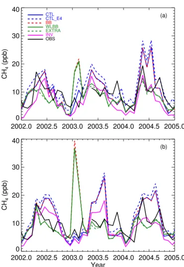
Figure 4. Monthly mean methane residuals for 2002–2004 at
Cape Grim for the observations (black) and six emission scenarios (colours shown in key):(a)ACCESS(b)CCAM. Note that the ob-servational mean residual for April 2003 is missing, due to lack of radon data with which to define the baseline threshold (rather than a lack of methane data).
cember 2002 to February 2003 and November 2006 to Jan-uary 2007, with very high peak CH4 concentrations for the
flux scenarios that included interannually varying biomass burning. The second feature was a large difference in CH4
concentrations in each winter between different flux scenar-ios.
01 02 03 04 05 06 07 08 09 10 11 12 13 14 15 16 17 18 19 20 21 22 23 24 25 26 27 28 29 30 31 0
20 40 60 80 100 120
CH
4
residuals (ppb)
AGAGE CH4
CTL WLBB
01 02 03 04 05 06 07 08 09 10 11 12 13 14 15 16 17 18 19 20 21 22 23 24 25 26 27 28 29 30 31 200
400 600
CO (ppb)
AGAGE CO
01 02 03 04 05 06 07 08 09 10 11 12 13 14 15 16 17 18 19 20 21 22 23 24 25 26 27 28 29 30 31 January 2003
500 550 600 650
H2
(ppb)
AGAGE H2
Figure 5.Cape Grim data for January 2003. Upper panel: observed
(black) CH4residuals; CCAM simulated residuals for tracers CTL (red) and WLBB (blue). Middle panel: observed CO. Lower panel: observed H2.
(WLBB and EXTRA) or based on the inversion of Bousquet et al. (2006) (INV).
4.1 Biomass burning
Figure 5 shows observed and CCAM simulated CH4
residuals for January 2003 as well as observed hydro-gen (H2) and carbon monoxide (CO). High H2 and CO
are signatures of air influenced by biomass burning. Two simulated CH4 tracers are shown, one which
in-cludes interannually varying biomass burning emissions (WLBB) and one that does not (CTL). The inclusion of “hot spots” of biomass burning emissions produces very large methane concentrations, much larger than those observed. Significant fires did occur during this period – in the eastern Victorian alpine region starting on 8 Jan-uary 2003 and burning around 1.3 million hectares over close to two months (http://www.depi.vic.gov.au/fire-
and-emergencies/managing-risk-and-learning-
about-managing-fire/bushfire-history/maps-of-past-bushfires) and around Canberra between 18 and 21 January 2003. The observations indicate that the Victorian fire was likely seen briefly at Cape Grim on 11 January, when CH4,
H2 and CO all had elevated concentrations. It is less clear
what contribution biomass burning makes to other elevated methane events later in the month, when only small CO elevations are seen and H2 signals do not rise above the
instrumental noise (except perhaps around 25 January). There are a number of reasons why the models may over-estimate the impact of this fire at Cape Grim. Firstly, the biomass burning emissions are specified at the middle of each month and interpolated to the middle of the previ-ous and following months. This means that a January fire is spread temporally into December and February. Indeed, WLBB also shows very large CH4concentrations in
Decem-ber 2002 and February 2003 (not shown). Secondly, the fire emissions were provided on a 1◦×
1◦
grid and have been re-gridded to the lower resolutions of the atmospheric models. In reality, the active fire at any given time would have covered a much smaller area. Finally, the fire itself would modify the local circulation, with emissions likely distributed not just near the surface but throughout the entire lower troposphere. This is not captured in our simulations where the emissions are input only to the lowest model level. For instance, Sofiev et al. (2013) find that, under Australian fire conditions, 90 % of mass is emitted from the surface up to 3 km altitude.
To test the sensitivity to the height that emissions are input to the atmosphere, we have performed some short tests, run-ning CCAM from December 2002 to February 2003, with only biomass burning emissions. Six tests were performed, releasing the emissions into model levels 1, 3, 5, 7 and 9 in turn (centred at approximately 40, 470, 1420, 2880, 4870 m respectively), or distributed through all levels 1–9. In general we find that the simulated timing of elevated CH4events at
Cape Grim is similar across the six tests but the amplitude of the events varies with emission insertion height. For ex-ample, the mean January CH4 concentration at Cape Grim
is reduced from 16 ppb for emissions inserted into level 1 to 12, 7, 2 and 0.3 ppb as emissions are input higher into the at-mosphere. For the case where emissions are spread between levels 1 and 9, the mean January CH4concentration is 5 ppb.
While these simulations (modelling only the biomass burn-ing component) are not directly comparable to the observa-tions, they clearly illustrate one reason why the amplitude of events at Cape Grim could be overestimated. The frequency of events appears to be more strongly controlled by the tem-poral and spatial (horizontal) resolution of the emissions.
4.2 Relationship between methane and radon: seasonal cycle
Given the variation in simulated winter CH4concentrations
by the very large concentrations caused by the interannu-ally varying biomass burning fluxes, we remove the biomass burning contribution from BB, WLBB and EXTRA for the months December 2002 to February 2003 and also Novem-ber 2006 to January 2007, when another large fire gives un-realistically high simulated concentrations of CH4 at Cape
Grim. This was achieved by subtracting (BB – CTL) from each of the three affected tracers, during the months in ques-tion.
To minimize the impact of any errors in modelled atmo-spheric transport, we consider the ratio of methane resid-ual concentrations to radon concentrations. The time series of methane residuals at Cape Grim is reasonably well cor-related with radon, with both showing significantly elevated concentrations when air parcels have travelled over continen-tal Australia. For the period 1994–2007, the correlation co-efficient between observed methane residuals and observed radon is 0.65. In the model simulations, correlations between residual methane and radon vary across methane scenarios between 0.81–0.87 for ACCESS and 0.88–0.89 for CCAM. The higher correlation coefficients for the modelled data set compared to the observed data set presumably reflect the re-duced spatial variability of both CH4and radon in the
grid-ded models compared to the real world.
The strategy of using a residual methane to radon ratio to minimize transport errors relies on the assumption that both sources are similarly distributed. We note that this assump-tion is only loosely true. The methane emission scenarios we assess here have considerable spatial variability (though doubtless less than the real world), while the TransCom-CH4-specified radon emissions are uniform over land. Land
surface emissions of radon do vary (Griffiths et al., 2010), though much less than for methane. As a check on our sensi-tivity to radon spatial variability, we ran ACCESS for 3 years using a series of different radon flux fields taken from Grif-fiths et al. (2010). In general, neither the spatial variability nor the interannual variability appeared to have a signifi-cant impact on our sampled concentrations at Cape Grim. We found that the choice of grid cell was much more influential in the modelled radon results matching the observed radon results, hence our choice of ocean grid cells to the north of Cape Grim. One of the reasons for this is likely to be the coarseness of the grid cells: see Sect. 3.2 and refer to the in-set in Fig. 1.
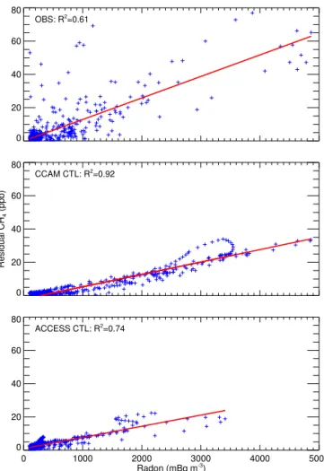
We examine the seasonal relationship between methane residuals and radon by fitting a linear relationship to all hourly non-baseline methane–radon pairs in a given month across the 14 years of the simulation for which we have observational data for comparison (1994–2007). For clarity, Fig. 6 shows this fit for a single month only, January 2006, for observations and modelled CTL cases. We take this approach in order to compare the observations to both the CCAM and ACCESS simulations. At the time of this work, ACCESS meteorology was forced only with sea surface temperatures and ran on a 360-day calendar, as described in Sect. 3. This
0 20 40 60 80
OBS: R2=0.61
0 20 40 60 80
Residual CH
4
(ppb)
CCAM CTL: R2=0.92
0 1000 2000 3000 4000 5000
Radon (mBq m-3) 0
20 40 60 80
ACCESS CTL: R2=0.74
Figure 6.Scatter plots of methane to radon, with linear fits for
Jan-uary 2006. The upper panel shows the observational data, the mid-dle panel the CCAM data and the lower panel the ACCESS data.
means that we do not expect the timing of individual “events” (non-baseline periods) in ACCESS to match the observations well enough for a direct comparison. We do however expect that the seasonal-scale meteorology will be realistic enough to provide seasonal fetch changes that are comparable to the real meteorology and fetch patterns at Cape Grim. Averaging results up to a seasonal timescale allows direct comparison of all three data sets (the observations and both models). The observations show more scatter than the model output, and this is reflected in lowerR2values, in this case 0.61 for the
observations and 0.92 and 0.74 for CCAM and ACCESS re-spectively. The slope of the line gives the methane residual to radon ratio. We determine the ratio this way to preserve the temporal pairing of the methane and radon concentra-tions. We also calculate linear fits for each individual month as per Fig. 6, and use the standard deviation of the slopes for each of the 14 months as a measure of the uncertainty on the methane–radon ratios.
win-0 5 10 15 20
CH
4
(ppb):Rn (Bq m
-3)
CTL
0 5 10 15 20
CTL_E4
0 5 10 15 20
CH
4
(ppb):Rn (Bq m
-3)
BB
0 5 10 15 20
WLBB
J F M A M J J A S O N D 0
5 10 15 20
CH
4
(ppb):Rn (Bq m
-3)
EXTRA
J F M A M J J A S O N D 0
5 10 15 20
INV
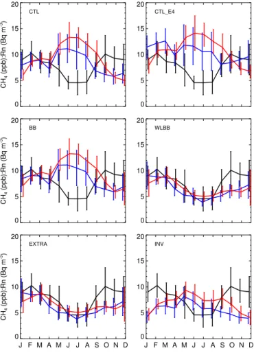
Figure 7.Mean seasonal cycle of residual methane to radon ratios
for each of the six methane emission scenarios. Observations are shown in black, ACCESS results in blue and CCAM results in red.
ter (June to August) and are largest in spring and summer (October to February). The modelled ratios show three pat-terns depending on the methane scenario. The CTL, CTL_E4 and BB scenarios show maximum ratios in winter, while the WLBB and EXTRA scenarios show minimum ratios in win-ter, which is more consistent with the observations. The INV scenario is intermediate between the other cases, also show-ing somewhat elevated winter ratios. For any given scenario, the ratios for the two different models compare well, much better than if either of the individual trace gases (methane or radon) are directly compared, as was the case in Fig. 4 where the monthly mean methane is shown for both models. This il-lustrates the benefit of using the radon simulation to account for some of the transport differences between the models.
Overall the WLBB and EXTRA scenarios give ratios that are a better fit to those observed. For the southeastern Aus-tralian region, the major difference from the group of CTL-based cases is in the representation of wetlands. These re-sults suggest that the large winter wetland fluxes in the CTL-based scenarios taken from Matthews and Fung (1987) and Fung et al. (1991) are not realistic and that annual mean fluxes should be close to the anthropogenic-only inventory
J F M A M J J A S O N D
0 5 10 15 20
CH
4
(ppb):Rn (Bq m
-3 )
Figure 8.Mean seasonal cycle of residual methane to radon ratios
for the CTL methane scenario (red, solid) and the CTL methane fluxes shifted forward in time by three months (red, dashed) com-pared to the observations (black). Both simulations used the CCAM model.
estimates noted in Sect. 3.1. For all scenarios (except perhaps CTL_E4) there is a discrepancy between the observed and modelled ratios in the austral spring (September to Novem-ber) with the observed ratios being larger than the modelled ones. This suggests that the methane flux scenarios tested here underestimate methane fluxes in spring. We will discuss this further in Sect. 5.
While the ratios from the CTL_E4 scenario agree rea-sonably with those observed in September–October, this oc-curs mainly because the CTL_E4 scenario gives generally higher ratios all year round compared to the CTL case. This is expected since the CTL_E4 fluxes for southeastern Aus-tralia gradually increase in time relative to the CTL fluxes (Fig. 3b). There is weak evidence of an increase in ratio over time for CTL_E4 compared to CTL but the large seasonal and interannual variability means that we can have little con-fidence in the calculated trends and which might compare better to the observations. The seasonality of ratios is similar between CTL and CTL_E4 (and a poor fit to observed sea-sonality) although the difference between summer and win-ter ratios is smaller in CTL_E4 especially in the ACCESS case. This may be due to changes in the spatial distribution of fluxes between CTL and CTL_E4. Overall CTL_E4 does not agree well with the observations.
5 Discussion and concluding remarks
fluxes. The WLBB and EXTRA flux scenarios appear to be the best fit to the observed data. Like Fraser et al. (2011), we find that anthropogenic methane emissions taken from inventories for southeastern Australia look quite reasonable in magnitude at around 2.5 Tg y−1. However, there remain questions about the scale and timing of a wetland component to CH4emissions.
Our analysis reveals that mismatches in the CTL, CTL_E4 and BB scenarios were due to high wetland emissions dur-ing the winter, suggestdur-ing that the wintertime wetland flux is overestimated in these scenarios. The Cape Grim observa-tions point to somewhat larger springtime fluxes than are rep-resented in the WLBB or EXTRA emission scenarios (or in-deed any of the other tracers). Although the wintertime max-ima of the CTL-style emission scenarios (driven by a wetland emission component) is clearly not warranted by the obser-vational data, a shift in the wetland emissions from austral winter to spring might result in a better fit to the observa-tions.
To test this we have run CCAM from December 1, 1993 to December 31, 2007 for radon and two methane scenar-ios, the standard CTL case and with the same CTL fluxes shifted forward in time by 3 months (across the whole globe). For southeastern Australia, this means that methane fluxes are elevated between August and January instead of between May and October. The output from the simulation has been processed similarly to the previous cases and Fig. 8 shows the seasonal cycle of methane-to-radon ratio. The case with temporally shifted fluxes clearly fits the observations better than the original CTL fluxes, although a 4-month shift in the fluxes might improve the comparison with observations fur-ther. The shifted fluxes case does not simulate a low enough methane minimum in winter. This may be a consequence of shifting the CTL fluxes across the whole globe rather than just for southeastern Australia. For example a large flux just to the north of the region we define occurs in February in the CTL fluxes and consequently gets shifted to May in the sensitivity test performed here. Nevertheless, this simulation supports the need for a shift in wetland emissions from aus-tral winter to spring and summer.
A shift of this nature is plausible given that wetland methane emissions have both a soil moisture and soil tem-perature dependence, making it possible that southeastern Australian methane emissions from wetlands are highest in springtime when there is available moisture and warmer tem-peratures. Indeed, Bloom et al. (2012) use satellite column observations of CH4 from the SCanning Imaging
Absorp-tion spectroMeter for Atmospheric CHartographY (SCIA-MACHY) coupled with a measure of equivalent water height from the Gravity Recovery and Climate Experiment (GRACE) to model seasonal variability in wetland methane emissions. For our region of interest across the years 2003– 2008, they find the minimum in methane emissions from southeastern Australian wetlands occurs in late autumn and winter with a rapid rise through spring giving a maximum
in October and November (A. Fraser, personal communica-tion, 2012) in accordance with the Cape Grim observations. However, the magnitude they predict for thiswetlandflux is around 2.5 Tg y−1. This seems larger than indicated by the Cape Grim data; of the six emission scenarios considered in this work, annual means fortotalCH4flux (including all
an-thropogenic emissions) in our defined region range between 2.4 (WLBB) and 4 (CTL) Tg y−1(Fig. 3b). Moreover, the ad-ditional 1.6 Tg y−1in the CTL emission scenario comes from a wintertime wetland flux that we find no evidence for in the observations. It should be noted however that in Fraser et al. (2011) the GRACE data used were scaled to match a prior emissions estimate. We therefore find that the GRACE data have plausible seasonality for southeastern Australia but that the magnitude is too large to offer a realistic assessment of the scale of southeastern Australian wetland emissions given the Cape Grim observations. Nevertheless, we believe the seasonality of the GRACE data lends credibility to the idea that a springtime wetland emission of around the magnitude represented in the CTL-style emissions scenarios for winter may be responsible for the discrepancy between our mod-elled WLBB/EXTRA results and the observations.
Although our hypothesis that the timing of wetland methane emissions in the inventories may be off by 3–4 months is plausible and supported by other data, we can-not entirely rule out acan-nother source for the additional aus-tral spring methane emissions. For instance, ruminant emis-sions from cattle are the single biggest contributor to Aus-tralia’s anthropogenic methane emissions. Seasonality in ru-minant emissions that is not captured by the inventories, due to changes in feed or cattle number, might also be responsi-ble for the austral springtime maximum observed. This ex-planation is offered in Wang and Bentley (2002) to account for a springtime spike in their estimated emissions from a region roughly equivalent to Victoria and New South Wales (their region D) when fitting the Cape Grim CH4data. While
this would concur with our results, overall Wang and Bent-ley (2002) find a significant reduction (around 40 %) in the inversion-estimated CH4 fluxes for southeastern Australia
compared to the 1997 inventory (Table 3). This does not agree with this work or with Fraser et al. (2011), which both suggest that the total methane emissions in the inven-tories for southeastern Australia are consistent with the Cape Grim data. The methodology in Wang and Bentley (2002) is to invert a series of 22 individual non-baseline “events” each lasting between 2 and 11 days. The inversion results for each event show considerable variability giving fluxes ranging from 0–7 Tg y−1 for region D. Such high
variabil-ity would appear to be unrealistic and may be caused by er-rors in the modelling of CH4concentration at Cape Grim for
a given Australian flux. Thus the inversion estimated fluxes are unlikely to be representative of the true flux.
of biomass burning emissions produces unrealistically high CH4concentrations at Cape Grim, but this is most likely due
to the coarse spatio-temporal resolution of the models and the unrealistic injection of these emissions into the lowest model level. In future, continuous CH4measurements made
from unmanned aerial vehicles (UAVs) around large fire plumes may be a better way to verify the scale of emissions from large biomass burning events. By comparing a range of methane emission scenarios run in the models, we find that the large wintertime wetland flux in the CTL-style sce-narios is unrealistic, but also that there is a deficit in spring in all six emission scenarios. This deficit is present in even the WLBB and EXTRA scenarios which otherwise provide a good fit to the observational data. It is notable that these two emission scenarios have a very small wetland emission component compared to the CTL-style scenarios. We sug-gest then, that it may be a springtime wetland emission that is missing from these scenarios. Finally, we note that given the size and uncertainty associated with the biogenic CH4
fluxes, it is difficult to make assessments about changes in anthropogenic CH4emissions in southeastern Australia from
the Cape Grim data set alone using this approach. Additional in situ instrumented sites for the continuous measurement of methane on the Australian mainland would help to answer questions about the scale and timing of wetland emissions as well as providing more stringent constraints on changes to the anthropogenic flux from southeastern Australia.
Acknowledgements. We thank AGAGE and Cape Grim staff, along with all the TransCom-CH4 participants, but in particular Prabir Patra for his efforts in setting up the experiment. This work has been undertaken as part of the Australian Climate Change Science Programme, funded jointly by the Department of the Environment, the Bureau of Meteorology and CSIRO. Model simulations were undertaken on the NCI National Facility in Canberra, Australia, which is supported by the Australian Commonwealth Government. We thank the reviewers for their helpful comments.
Edited by: P. Monks
References
Aoki, S., Nakazawa, T., Murayama, S., and Kawaguchi, S.: Mea-surements of atmospheric methane at the Japanese Antarctic sta-tion, Syowa, Tellus B, 44, 273–281, 1992.
Biraud, S., Ciais, P., Ramonet, M., Simmonds, P., Kazan, V., Mon-fray, P., O’Doherty, S., Spain, T. G., and Jennings, S. G.: Euro-pean greenhouse gas emissions estimated from continuous atmo-spheric measurements and radon 222 at Mace Head, Ireland, J. Geophys. Res., 105, 1351–1366, 2000.
Bloom, A. A., Palmer, P. I., Fraser, A., and Reay, D. S.: Sea-sonal variability of tropical wetland CH4emissions: the role of the methanogen-available carbon pool, Biogeosciences, 9, 2821– 2830, doi:10.5194/bg-9-2821-2012, 2012.
Bousquet, P., Ciais, P., Miller, J. B., Dlugokencky, E. J., Hauglus-taine, D. A., Prigent, C., Van der Werf, G. R., Peylin, P., Brunke, E. G., Carouge, C., Langenfelds, R. L., Lathière, J., Papa, F., Ramonet, M., Schmidt, M., Steele, L. P., Tyler, S. C., and White, J.: Contribution of anthropogenic and natural sources to atmospheric methane variability, Nature, 443, 439–443, doi:10.1038/nature05132, 2006.
Bousquet, P., Ringeval, B., Pison, I., Dlugokencky, E. J., Brunke, E.-G., Carouge, C., Chevallier, F., Fortems-Cheiney, A., Franken-berg, C., Hauglustaine, D. A., Krummel, P. B., Langen-felds, R. L., Ramonet, M., Schmidt, M., Steele, L. P., Szopa, S., Yver, C., Viovy, N., and Ciais, P.: Source attribution of the changes in atmospheric methane for 2006–2008, Atmos. Chem. Phys., 11, 3689–3700, doi:10.5194/acp-11-3689-2011, 2011. Chambers, S., Williams, A. G., Zahorowski, W., Griffiths, A., and
Crawford, J.: Separating remote fetch and local mixing influ-ences on vertical radon measurements in the lower atmosphere, Tellus B, 63, 843–859, doi:10.1111/j.1600-0889.2011.00565.x, 2011.
Collier, M. A.: The CSIRO NCEP/NCAR/DOER-1/R-2archive, CSIRO Atmospheric Research technical paper 68, Aspendale, Victoria, Australia, available at: http://www.cmar.csiro.au/ e-print/open/collier_2004a.pdf, 2004.
Corbin, K. D. and Law, R. M.: Extending atmospheric CO2 and tracer capabilities in ACCESS, CAWCR Technical Report 035, Aspendale, Victoria, Australia, available at: http://www.cawcr. gov.au/publications/technicalreports/CTR_035.pdf, 2011. Cunnold, D., Steele, L., Fraser, P., Simmonds, P., Prinn, R.,
Weiss, R., Porter, L., O’Doherty, S., Langenfelds, R., Krum-mel, P., Wang, H., Emmons, L., Tie, X., and Dlugokencky, E.: In situ measurements of atmospheric methane at GAGE/AGAGE sites during 1985–2000 and resulting source inferences, J. Geophys. Res.-Atmos., 107, 4225, doi:10.1029/2001JD001226, 2002.
Dlugokencky, E. J., Bruhwiler, L., White, J. W. C., Emmons, L. K., Novelli, P. C., Montzka, S. A., Masarie, K. A., Lang, P. M., Crotwell, A. M., Miller, J. B., and Gatti, L. V.: Observational constraints on recent increases in the atmospheric CH4burden, Geophys. Res. Lett., 36, L18803, doi:10.1029/2009GL039780, 2009.
Fraser, A., Chan Miller, C., Palmer, P. I., Deutscher, N. M., Jones, N. B., and Griffith, D. W. T.: The Australian methane budget: interpreting surface and train-borne measurements us-ing a chemistry transport model, J. Geophys. Res., 116, D20306, doi:10.1029/2011JD015964, 2011.
Fung, I., John, J., Lerner, J., Matthews, E., Prather, M., Steele, L. P., and Fraser, P. J.: Three-dimensional model synthesis of the global methane cycle, J. Geophys. Res., 96, 13033–13065, 1991. Griffiths, A. D., Zahorowski, W., Element, A., and Werczynski, S.:
A map of radon flux at the Australian land surface, Atmos. Chem. Phys., 10, 8969–8982, doi:10.5194/acp-10-8969-2010, 2010. Houweling, S., Kaminski, T., Dentener, F., Lelieveld, J., and
Heimann, M.: Inverse modeling of methane sources and sinks using the adjoint of a global transport model, J. Geophys. Res., 104, 26137–26160, 1999.
Kalnay, E., Kanamitsu, M., Kistler, R., Collins, W., Deaven, D., Gandin, L., Iredell, M., Saha, S., White, G., Woollen, J., Zhu, Y., Chelliah, M., Ebisuzaki, W., Higgins, W., Janowiak, J., Mo, K., Ropelewski, C., Wang, J., Leetmaa, A., Reynolds, R., Jenne, R., and Jospher, D.: The NCEP/NCAR 40-year reanalysis project, B. Am. Meteorol. Soc., 77, 437–471, 1996.
Kirschke, S., Bousquet, P., Ciais, P., Saunois, M., Canadell, J. G., Dlugokencky, E. J., Bergamaschi, P., Bergmann, D., Blake, D. R., Bruhwiler, L., Cameron-Smith, P., Castaldi, S., Chevallier, F., Feng, L., Fraser, A., Heimann, M., Hodson, E. L., Houweling, S., Josse, B., Fraser, P. J., Krummel, P. B., Lamarque, J.-F., Langen-felds, R. L., Le Quéré, C., Naik, V., O’Doherty, S., Palmer, P. I., Pison, I., Plummer, D., Poulter, B., Prinn, R. G., Rigby, M., Ringeval, B., Santini, M., Schmidt, M., Shindell, D. T., Simp-son, I. J., Spahni, R., Steele, L. P., Strode, S. A., Sudo, K., Szopa, S., van der Werf, G. R., Voulgarakis, A., van Weele, M., Weiss, R. F., Williams, J. E., and Zeng, G.: Three decades of global methane sources and sinks, Nat. Geosci., 6, 813–823, doi:10.1038/NGEO1955, 2013.
Krummel, P., Fraser, P., Steele, L., Derek, N., Rickard, C., Ward, J., Somerville, N. T., Cleland, S. J., Dunse, B., Langenfelds, R., Baly, S. B., and Leist, M.: The AGAGE in situ program for non-CO2greenhouse gases at Cape Grim, 2009–2010, in: Base-line Atmospheric Program (Australia), 2009–2010, edited by: Derek, N., Krummel, P. B., and Cleland, S. J., Australian Bureau of Meteorology and CSIRO Marine and Atmospheric Research, Aspendale, Victoria, Australia, 56–70, 2014.
Langenfelds, R., Steele, L., Gregory, R. L., Krummel, P., Spencer, D., and Howden, R.: Atmospheric methane, carbon dioxide, hydrogen, carbon monoxide and nitrous oxide from Cape Grim flask air samples analysed by gas chromatography, in: Baseline Atmospheric Program (Australia), 2009–2010, edited by: Derek, N., Krummel, P. B., and Cleland, S. J., Australian Bu-reau of Meteorology and CSIRO Marine and Atmospheric Re-search, Aspendale, Victoria, Australia, 45–49, 2014.
MacFarling Meure, C., Etheridge, D., Trudinger, C., Steele, P., Langenfelds, R., van Ommen, T., Smith, A., and Elkins, J.: Law dome CO2, CH4 and N2O ice core records ex-tended to 2000 years BP, Geophys. Res. Lett., 33, L14810, doi:10.1029/2006GL026152, 2006.
Matthews, E. and Fung, I.: Methane emission from natural wetlands: global distribution, area, and environmental char-acteristics of sources, Global Biogeochem. Cy., 1, 61–86, doi:10.1029/GB001i001p00061, 1987.
McGregor, J. L.: C-CAM: Geometric aspects and dynamical formu-lation, CSIRO Atmospheric Research Technical Paper 70, As-pendale, Victoria, Australia, available at: http://www.cmar.csiro. au/e-print/open/mcgregor_2005a.pdf, 2005.
McGregor, J. L. and Dix, M. R.: An updated description of the Con-formal Cubic Atmospheric Model, in: High Resolution Numeri-cal Modelling of the Atmosphere and Ocean, edited by: Hamil-ton, K. and Ohfuchi, W., Springer, Berlin, 51–76, 2008. Miller, S. M., Wofsy, S. C., Michalak, A. M., Kort, E. A.,
Andrews, A. E., Biraud, S. C., Dlugokencky, E. J., Eluszkiewicz, J., Fischer, M. L., Janssens-Maenhout, G., Miller, B. R., Miller, J. B., Montzka, S. A., Nehrkorn, T., and Sweeney, C.: Anthropogenic emissions of methane in the United States, P. Natl. Acad. Sci. USA, 110, 20018–20022, doi:10.1073/pnas.1314392110, 2013.
Olivier, J. G. J. and Berdowski, J. J. M.: Global emissions sources and sinks, in: The Climate System, edited by: Berdowski, J. J. M., Guicherit, R., and Heij, B. J., A. A. Balkema Publishers/Swets & Zeitlinger Publishers, Lisse, The Netherlands, 33–78, 2001. Olivier, J. G. J., van Aardenne, J. A., Dentener, F., Ganzeveld, L.,
and Peters, J. A. H. W.: Recent trends in global greenhouse gas emissions: regional trends and spatial distribution of key sources, in: Non-CO2Greenhouse Gases (NCGG-4), edited by: van Am-stel, A., Millpress, Rotterdam, 325–330, 2005.
Patra, P. K., Houweling, S., Krol, M., Bousquet, P., Bruhwiler, L., and Jacob, D.: Protocol for TransCom CH4 intercompari-son, Version 7, available at: http://transcom.project.asu.edu/ pdf/transcom/T4.methane.protocol_v7.pdf (last access: August 2014), 2010.
Patra, P. K., Houweling, S., Krol, M., Bousquet, P., Belikov, D., Bergmann, D., Bian, H., Cameron-Smith, P., Chipperfield, M. P., Corbin, K., Fortems-Cheiney, A., Fraser, A., Gloor, E., Hess, P., Ito, A., Kawa, S. R., Law, R. M., Loh, Z., Maksyutov, S., Meng, L., Palmer, P. I., Prinn, R. G., Rigby, M., Saito, R., and Wilson, C.: TransCom model simulations of CH4 and re-lated species: linking transport, surface flux and chemical loss with CH4variability in the troposphere and lower stratosphere, Atmos. Chem. Phys., 11, 12813–12837, doi:10.5194/acp-11-12813-2011, 2011.
Prinn, R., Weiss, R., Fraser, P., Simmonds, P., Cunnold, D., Alyea, F., O’Doherty, S., Salameh, P., Miller, B., Huang, J., Wang, R., Hartley, D., Harth, C., Steele, L., Sturrock, G., Midgley, P., and McCulloch, A.: A history of chemi-cally and radiatively important gases in air deduced from ALE/GAGE/AGAGE, J. Geophys. Res.-Atmos., 105, 17751– 17792, doi:10.1029/2000JD900141, 2000.
Rigby, M., Prinn, R. G., Fraser, P. J., Simmonds, P. G., Lan-genfelds, R. L., Huang, J., Cunnold, D. M., Steele, L. P., Krummel, P. B., Weiss, R. F., O’Doherty, S., Salameh, P. K., Wang, H. J., Harth, C. M., Muehle, J., and Porter, L. W.: Re-newed growth of atmospheric methane, Geophys. Res. Lett., 35, L22805, doi:10.1029/2008GL036037, 2008.
Ringeval, B., de Noblet-Ducoudré, N., Ciais, P., Bousquet, P., Pri-gent, C., Papa, F., and Rossow, W. B.: An attempt to quantify the impact of changes in wetland extent on methane emissions on the seasonal and interannual time scales, Global Biogeochem. Cy., 24, GB2003, doi:10.1029/2008GB003354, 2010.
Schmidt, M., Graul, R., Sartorius, H., and Levin, I.: Carbon diox-ide and methane in continental Europe: a climatology, and 222Radon-based emission estimates, Tellus B, 48, 457–473,
1996.
Sofiev, M., Vankevich, R., Ermakova, T., and Hakkarainen, J.: Global mapping of maximum emission heights and resulting vertical profiles of wildfire emissions, Atmos. Chem. Phys., 13, 7039–7052, doi:10.5194/acp-13-7039-2013, 2013.
Sussmann, R., Forster, F., Rettinger, M., and Bousquet, P.: Renewed methane increase for five years (2007–2011) observed by so-lar FTIR spectrometry, Atmos. Chem. Phys., 12, 4885–4891, doi:10.5194/acp-12-4885-2012, 2012.
Thatcher, M. J. and McGregor, J. L.: Using a scale-selective fil-ter for dynamical downscaling with the Conformal Cubic Atmo-spheric Model, Mon. Weather Rev., 137, 1742–1752, 2009. Thoning, K. W., Tans, P. P., and Komhyr, W. D.: Atmospheric
NOAA/GMCC data, 1974–1985, J. Geophys. Res., 94, 8549– 8565, 1989.
van Aardenne, J. A., Dentener, F. J., Olivier, J. G. J., Klein Gold-ewijk, C. G. M., and Lelieveld, J.: A 1◦×1◦resolution data set of historical anthropogenic trace gas emissions for the period 1890– 1990, J. Geophys. Res., 15, 909–928, 2001.
van der Werf, G. R., Randerson, J. T., Giglio, L., Collatz, G. J., Kasibhatla, P. S., and Arellano Jr., A. F.: Interannual variabil-ity in global biomass burning emissions from 1997 to 2004, At-mos. Chem. Phys., 6, 3423–3441, doi:10.5194/acp-6-3423-2006, 2006.
Wada, A., Matsueda, H., Murayama, S., Taguchi, S., Hirao, S., Ya-mazawa, H., Moriizumi, J., Tsuboi, K., Niwa, Y., and Sawa, Y.: Quantification of emission estimates of CO2, CH4 and CO for East Asia derived from atmospheric radon-222 measure-ments over the western North Pacific, Tellus B, 65, 18037, doi:10.3402/tellusb.v65i0.18037, 2013.
Wang, Y. P. and Bentley, S. T.: Development of a spatially explicit inventory of methane emissions from Australia and its verifica-tion using atmospheric concentraverifica-tion data, Atmos. Environ., 36, 4965–4975, 2002.
Whittlestone, S. and Zahorowski, W.: The Cape Grim Huge Radon detector, in: Baseline Atmospheric Program (Australia) 92, edited by: Dick, A. L. and Fraser, P. J., Australian Bureau of Meteorology and CSIRO Marine and Atmospheric Research, As-pendale, Victoria, Australia, 26–30, 1995.
Whittlestone, S. and Zahorowski, W.: Baseline radon detectors for shipboard use: development and deployment in the First Aerosol Characterisation experiment (ACE 1), J. Geophys. Res., 103, 16743–16751, 1998.
Williams, A. G., Zahorowski, W., Chambers, S., Griffiths, A., Hacker, J. M., Element, A., and Werczynski, S.: The ver-tical distribution of radon in clear and cloudy daytime terrestrial boundary layers, J. Atmos. Sci., 68, 155–174, doi:10.1175/2010JAS3576.1, 2011.
Williams, A. G., Chambers, S., and Griffiths, A.: Bulk mixing and decoupling of the nocturnal stable boundary layer characterized using a ubiquitous natural tracer, Bound.-Lay. Meteorol., 149, 381–402, doi:10.1007/s10546-013-9849-3, 2013.
Wilson, S., Dick, A., Fraser, P., and Whittlestone, S.: Nitrous oxide flux estimates for South-Eastern Australia, J. Atmos. Chem., 26, 169–188, 1997.
Yan, X., Akiyama, H., Yagi, K., and Akimoto, H.: Global esti-mations of the inventory and mitigation potential of methane emissions from rice cultivation conducted using the 2006 Inter-governmental Panel on Climate Change Guidelines, Global Bio-geochem. Cy., 23, GB2002, doi:10.1029/2008GB003299, 2009. Zahorowski, W., Chambers, S. D., and Henderson-Sellers, A.: Ground based radon-222 observations and their application to atmospheric studies, J. Environ. Radioact., 76, 3–33, 2004. Zahorowski, W., Williams, A. G., Chambers, S. D., Crawford, J.,