On the interest of positive degree day models for mass balance modeling in the inner tropics

(1)

TCD

8, 2637–2684, 2014

On the interest of positive degree day

models for mass balance modeling in

the inner tropics

L. Maisincho et al.

Title Page

Abstract Introduction

Conclusions References

Tables Figures

◭ ◮

Back Close

Full Screen / Esc

Printer-friendly Version

Interactive Discussion

Discussion

P

a

per

|

Discus

sion

P

a

per

|

Discussion

P

a

per

|

Discussion

P

a

per

|

The Cryosphere Discuss., 8, 2637–2684, 2014 www.the-cryosphere-discuss.net/8/2637/2014/ doi:10.5194/tcd-8-2637-2014

This discussion paper is/has been under review for the journal The Cryosphere (TC). Please refer to the corresponding final paper in TC if available.

On the interest of positive degree day

models for mass balance modeling in the

inner tropics

L. Maisincho1,2, V. Favier3, P. Wagnon2,4, R. Basantes Serrano2,3, B. Francou2, M. Villacis5, A. Rabatel3, L. Mourre2, V. Jomelli6, and B. Cáceres1

1

INAMHI, Instituto Nacional de Meteorología e Hidrología, Iñaquito N36-14 y Corea, Quito, Ecuador

2

Univ. Grenoble Alpes, CNRS, IRD, LTHE (UMR5564), 38000 Grenoble, France

3

Univ. Grenoble Alpes, CNRS LGGE (UMR5183), 38000 Grenoble, France

4

ICIMOD, G.P.O. Box 3226, Kathmandu, Nepal

5

EPN, Escuela Politécnica Nacional, Ladrón de Guevara E11-253, Quito, Ecuador

6

LGP, Université Paris 1 Panthéon-Sorbonne-CNRS, 92195 Meudon, France

Received: 1 April 2014 – Accepted: 6 May 2014 – Published: 23 May 2014

Correspondence to: L. Maisincho (lmaisincho@yahoo.com)

(2)

TCD

8, 2637–2684, 2014

L. Maisincho et al.

Title Page

Tables Figures

◭ ◮

Back Close

Full Screen / Esc

Discussion

P

a

per

|

Discus

sion

P

a

per

|

Discussion

P

a

per

|

Discussion

P

a

per

|

Abstract

A positive degree-day (PDD) model was tested on Antizana Glacier 15α (0.28 km2; 0◦28′S, 78◦09′W) to assess to what extent this approach is suitable for studying glacier mass balance in the inner tropics. Cumulative positive temperatures were compared with field measurements of melting amount and with surface energy balance

computa-5

tions. A significant link was revealed when a distinction was made between the snow and ice comprising the glacier surface. Significant correlations allowed degree-day fac-tors to be retrieved for snow, and clean and dirty ice. The relationship between melt amount and temperature was mainly explained by the role of net shortwave radiation in both melting and in the variations in the temperature of the surface layer. However, this

10

relationship disappeared from June to October (Period 1), because high wind speeds and low humidity cause highly negative turbulent latent heat fluxes. However, this had little impact on the computed total amount of melting at the annual time scale because temperatures are low and melting is generally limited during Period 1. At the daily time scale, melting starts when daily temperature means are still negative, because

15

around noon incoming shortwave radiation is very high, and compensates for energy losses when the air is cold. The PDD model was applied to the 2000–2008 period us-ing meteorological inputs measured on the glacier foreland. Results were compared to the glacier-wide mass balances measured in the field and were good, even though the melting factor should be adapted to the glacier surface state and may vary with

20

(3)

TCD

8, 2637–2684, 2014

L. Maisincho et al.

Title Page

Tables Figures

◭ ◮

Back Close

Full Screen / Esc

Discussion

P

a

per

|

Discus

sion

P

a

per

|

Discussion

P

a

per

|

Discussion

P

a

per

|

1 Introduction

In recent decades, hydro-glacio-meteorological monitoring programs have been con-ducted to improve our understanding of current climate change in the high elevation Andes and to more accurately estimate its impact on ice-covered areas (e.g., Has-tenrath, 1981; Hastenrath and Kruss, 1992; Francou et al., 1995, 2000; Kaser and

5

Osmaston, 2002; Rabatel et al., 2013). In Ecuador, glaciological studies began on An-tizana Glacier 15α in 1994 (Francou et al., 2000; Favier et al., 2004a). Ecuadorian glaciers respond rapidly to climate change, in particular to temperature variations. The comparison of glacier extents using photogrammetric information available since 1956 (Francou et al., 2000; Basantes Serrano et al., 2014) with local variations in

temper-10

ature suggests that local warming of the atmosphere (about 0.2◦C decade−1, Vuille et al., 2000) has played an important role in glacier retreat since the 1950s (Francou et al., 2000), with direct consequences for the local water supply to Quito (e.g., Favier et al., 2008; Villacis, 2008). Temperature changes are generally assumed to be the main parameter involved in glacier retreat in the Ecuadorian Andes because the 0◦C

15

level oscillates continuously around the ablation zone average altitude throughout the year (Kaser, 2001; Favier et al., 2004a, b; Francou et al., 2004; Rabatel et al., 2013). Slight changes in temperature directly modify the ablation processes at the glacier sur-face due to the precipitation phase and its impact on the sursur-face albedo (e.g., Francou et al., 2004; Favier et al., 2004a). For instance, El Nino events lead to the rise of the

20

0◦C level, and therewith have major consequences for the precipitation phase over the glacier, leading to high melting rates (e.g., Francou et al., 2004; Favier et al., 2004b). However, a direct link between higher temperature and increased ablation has never been clearly demonstrated. Because the warming expected in the high elevation Andes in the 21st century (between 4 and 5◦C) (Bradley et al., 2006; Vuille et al., 2008; Urrutia

25

(4)

TCD

8, 2637–2684, 2014

L. Maisincho et al.

Title Page

Tables Figures

◭ ◮

Back Close

Full Screen / Esc

Discussion

P

a

per

|

Discus

sion

P

a

per

|

Discussion

P

a

per

|

Discussion

P

a

per

|

crucial, but first, we need to show that empirical approaches based on the relationship between temperature and melting are appropriate.

Positive degree-day (PDD) models (e.g., Braithwaite, 1995; Hock, 2003) have been widely used in tropical areas to study past glacier length fluctuations (e.g., Hostettler and Clark, 2000; Blard et al., 2007; Jomelli et al., 2011). The physical basis for the PDD

5

model is that net longwave radiation, sensible heat flux, and to a certain extent, the la-tent heat flux over a melting ice surface are significantly correlated with air temperature (Ohmura, 2001). The PDD model should also be applied in climatic zones with a well-defined annual air temperature cycle (Ohmura, 2001), i.e. outside the tropics. Sicart et al. (2008) suggested that PDD models should be used with caution even in the

trop-10

ics because temperature is not directly linked to the main local ablation processes. These authors argued that the shortwave radiation budget is the main process that de-termines the annual surface mass balance (Wagnon et al., 1999; Favier et al., 2004a, b; Sicart et al., 2008), and that the turbulent sensible heat flux and incoming longwave radiation are generally of less importance, with a low correlation between temperature

15

and melting processes. However, the study by Sicart et al. (2008) in the Andes was mainly based on data collected on Zongo Glacier, which is in the outer tropics (e.g., Kaser, 2001), whereas the inner tropics were only briefly analyzed. Sicart et al. (2008) used a 6 month dataset (September to February), but not a full annual cycle, whereas, unlike in the outer tropics, in Ecuador, a melting season is hard to define (e.g., Kaser

20

and Osmaston, 2002). Moreover, in their correlation analysis Sicart et al. did not dis-tinguish between snow and ice, whereas degree-day factors (DDF) are expected to be very di_fferent for the two surface states (e.g., Braithwaite, 1995). Finally, their analysis did not include direct field measurements of specific snow and ice melt to assess melt factors. Therefore, their conclusions concerning the inner tropics cannot be considered

25

definitive and a specific focus there is still necessary.

(5)

TCD

8, 2637–2684, 2014

L. Maisincho et al.

Title Page

Tables Figures

◭ ◮

Back Close

Full Screen / Esc

Discussion

P

a

per

|

Discus

sion

P

a

per

|

Discussion

P

a

per

|

Discussion

P

a

per

|

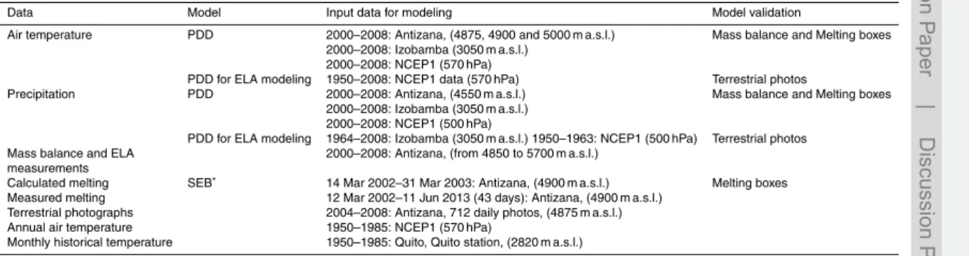
the field in 2002–2003 (Favier et al., 2004a) to analyze the capability of PDD mod-els to accurately reproduce measured melting values. We also used the computed melting values from energy balance calculations by Favier et al. (2004a) and surface mass balance and equilibrium-line altitude (ELA) data from the GLACIOCLIM observa-tory (http://www-lgge.ujf-grenoble.fr/ServiceObs/). We compared the distributed PDD

5

model results with continuous snowline observations obtained with an automatic cam-era since 2004 to check whether this variable was correctly reproduced. Finally, a criti-cal analysis of the sensitivity and limitations of the model was performed.

The paper is organized as follows: in Sect. 2, we provide a description of the regional climatic conditions; in Sect. 3, we describe the data and methods used. In Sect. 4, we

10

calibrate PDD model parameters using local melting measurements, and apply the model using meteorological datasets from different sources (from a local and a remote meteorological station, and then from reanalysis data). In Sect. 5, we describe model sensitivity. In Sect. 6, we discuss our results and examine when and how the PDD model should be used in the inner tropics.

15

2 Study site, climatic setting and associated glaciological processes

Antizana stratovolcano is one of the main ice covered summits in the Cordillera Oriental of Ecuador (Fig. 1). The last glacier inventory performed in 2006 showed that glaciers extended over a surface area of 12.2 km2 (Cáceres et al., 2006) distributed over 17 glacier tongues (Hastenrath, 1981). Glaciological and hydrological studies in the area

20

began in 1994 on Antizana Glacier 15α. This glacier is located on the north-western side of the volcano and is a reference site for long-term observations (Francou et al., 2000, 2004; Favier et al., 2004a, 2008; Rabatel et al., 2013). The surface of the glacier presently extends from 5700 m a.s.l. down to 4850 m a.s.l.

The study area belongs to the inner tropics, which are characterized by low

tem-25

(6)

TCD

8, 2637–2684, 2014

L. Maisincho et al.

Title Page

Tables Figures

◭ ◮

Back Close

Full Screen / Esc

Discussion

P

a

per

|

Discus

sion

P

a

per

|

Discussion

P

a

per

|

Discussion

P

a

per

|

temperatures over one year. The annual precipitation recorded at 4550 m a.s.l. in the catchment of Antizana 15 Glacier ranged from 800 to 1300 mm a−1between 2000 and 2008. Precipitation is significant throughout the year; monthly variations showed two slight maxima in April and October, while slight minima appeared in July–August and December (Favier et al., 2004a). As a consequence of these peculiar climatic

set-5

tings, accumulation and ablation occur simultaneously and continuously. The mean 0◦C level is generally around 4950–5000 m a.s.l., i.e. within the ablation zone. How-ever, this value shows large interannual variability. Consequently, liquid and solid pre-cipitation is frequent in the ablation area, and glaciological processes indirectly depend on temperature, because temperature directly controls the precipitation phase, and

10

hence temperature acts on surface albedo (Favier et al., 2004a). On the other hand, during the period 2000–2008, wind velocity showed pronounced seasonal variations, with intense easterly winds generally occurring between June and October (hereafter referred to as Period 1, while Period 2 refers to the period from November to May of the following year), which were associated with marked mass and energy losses through

15

sublimation (Favier et al., 2004a).

Finally, most local climate variability is closely linked to the El Niño–Southern Oscil-lation (ENSO). There is a three month delay in the local response of the atmosphere to the ENSO signal. ENSO warm phases (El Niño) are associated with local warming and a precipitation deficit leading to highly negative mass balances (Francou et al.,

20

2004; Favier et al., 2008). Conversely, La Niña phases are colder and more humid, which results in more balanced or even positive mass budgets. Surface energy bal-ance studies showed that these variations are closely linked with variations in albedo that mirror changes in the precipitation phase at the glacier surface due to variations in temperature.

(7)

TCD

8, 2637–2684, 2014

L. Maisincho et al.

Title Page

Tables Figures

◭ ◮

Back Close

Full Screen / Esc

Discussion

P

a

per

|

Discus

sion

P

a

per

|

Discussion

P

a

per

|

Discussion

P

a

per

|

3 Methods and data

3.1 The positive degree-day model

In this paper, we test a simple PDD model that allows calculation of daily snow or ice melta_j(z) (in mm w.e.) at a given elevation z (in m a.s.l.), and at time stepj (in days) (Braithwaite, 1995; Hock, 2003):

5

a_j(z)=−F(T_j(zref)+LR(z−zref)−Tthreshold) ifTj(zref)+LR(z−zref)> Tthreshold, (1)

aj(z)=0 ifTj(zref)+LR(z−zref)≤Tthreshold, (2)

whereF is the degree-day factor (DDF, in mm.w.e. K−1d−1), T_j(z) (in◦C) is the mean daily temperature,zref=4900 m a.s.l. andz(in m a.s.l.) are the reference elevation and

10

the given elevation respectively,Tthreshold(in

◦

C) is a threshold temperature above which melting begins, and LR is the lapse rate in the atmosphere (in◦C m−1, hereafter ex-pressed in◦C km−1). The PDD model generally assumes thatTthreshold=0

◦

C. However, during short periods in the daytime, melting may occur when a negative daily mean is observed (e.g. Van den Broeke et al., 2010). To avoid this problem, and as

recom-15

mended in several studies (e.g. Van den Broeke et al., 2010), the model was first ap-plied using cumulative amounts of positive temperature for each day, computed using hourly temperature values. However, because hourly temperatures are rarely available in long-term meteorological observations, we also applied the PDD model using daily mean temperature values, in this case assuming a negative Tthreshold=−1.9

◦

C (see

20

Sect. 4.2).

The model can be run using different DDF values depending on the presence or absence of snow at the glacier surface at the previous time step, whereSj−1(z) is the

amount of snow in mm.w.e. at the time stepj−1:

F =Fsnow ifSj−1(z)>0 (in mm.w.e. K−1d−1) (3)

25

(8)

TCD

8, 2637–2684, 2014

L. Maisincho et al.

Title Page

Tables Figures

◭ ◮

Back Close

Full Screen / Esc

Discussion

P

a

per

|

Discus

sion

P

a

per

|

Discussion

P

a

per

|

Discussion

P

a

per

|

Snow cover is the difference between ablation and snow accumulation at a given elevationz. Solid precipitation is assumed if the air temperature is below a threshold (Tsnow/rain=1

◦

C, Azam et al., 2014), otherwise solid precipitation is zero. This thresh-old was obtained from field measurements and direct observations of the precipitation phase in the Andes, which suggested that, below this temperature, more than 70 %

5

of precipitation is solid (e.g., L’Hôte et al., 2005). We assumed that total precipitation is constant with elevation. Temperature at a specific elevation is computed assuming a constant lapse rate (LR) between the reference elevationzref, where meteorological

data are available, and a given elevationz. A value of LR=−6.5◦C km−1(e.g., Rojas, 2006) is generally assumed in the free atmosphere. However, half-hourly field

temper-10

ature measurements performed in artificially ventilated shelters at different elevations on Antizana Glacier 12 (2 km south of the Antizana Glacier 15α) suggested a mean lapse rate of−8.0◦C km−1 (standard deviation of 3.0◦C km−1for 18 685 values) (data not shown). This vertical temperature gradient is higher than the humid adiabatic gra-dient because Glacier 12 and 15 are located on the leeward side of the volcano, where

15

there is a strong foehn effect that acts to steepen the vertical temperature gradient (e.g., Favier et al., 2004a). We use the latter value in the present paper, and a model sensitivity test against this parameter is presented in Sect. 5.

The elevation of the snowline zSL,j was estimated using the model and compared

with field observations. The modeled snowline is the level at which the snow

accumu-20

lation given by the model becomes positive. Finally, in the model, the ELA is the altitude at which the annual surface mass balanceb_j(z) is zero.

3.2 Surface energy balance computation

Daily ablation from the PDD model was compared with surface energy balance values given by Favier et al. (2004a, b). The energy stored in the top layers of the glacier∆Q

25

(9)

TCD

8, 2637–2684, 2014

L. Maisincho et al.

Title Page

Tables Figures

◭ ◮

Back Close

Full Screen / Esc

Discussion

P

a

per

|

Discus

sion

P

a

per

|

Discussion

P

a

per

|

Discussion

P

a

per

|

2011):

∆Q=S↓(1−α)+L↓₊L↑₊H+LE (in W m−2). (5)

Where, S↓is incident short-wave radiation,α is the albedo,L↓ andL↑are incom-ing and outgoincom-ing long-wave radiation, respectively, and H and LE are turbulent

sen-5

sible and latent heat fluxes, respectively. Conduction into the ice/snow or heat sup-plied by precipitation was ignored. When the surface temperature is at melting point,

∆Q represents the energy available for melt. The radiative fluxes were measured lo-cally at 4900 m a.s.l. on Antizana 15αwith a CNR1 Kipp&Zonen net radiometer. Turbu-lent fluxes were computed using the bulk aerodynamic approach assuming roughness

10

lengths obtained through measurements of sublimation in the field. Temperature and humidity were measured using an artificially ventilated HMP45 Vaisala sensor and wind speed was measured using a Young 05103 anemometer. See Favier et al. (2004a) for details.

3.3 Data

15

3.3.1 Meteorological data

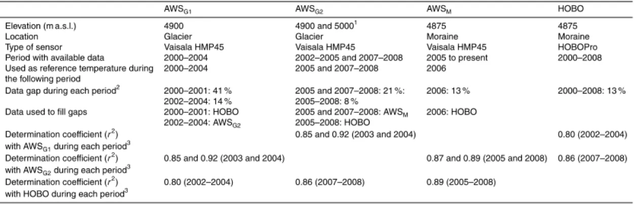
In this paper, we use data from four meteorological stations (Table 2) and two tipping bucket rain gauges (Table 1). The reference temperature used in our calculation is the value measured on the glacier at 4900 m a.s.l. The data and periods used in this paper (Table 3) are the following:

20

1. meteorological datasets recorded by the AWSG1 (Fig. 1) automatic weather

sta-tion (AWS, hereafter referred to as AWSG1, 4900 m a.s.l.) between 1999 to 2004.

The subindex G1 in AWS_G1 means glacier. The sensors installed on the AWS_G1 and the available data are the same as described in Favier et al. (2004a, b). Ta-ble 1 summarizes the observed variaTa-bles and sensor characteristics for the period

25

(10)

TCD

8, 2637–2684, 2014

L. Maisincho et al.

Title Page

Tables Figures

◭ ◮

Back Close

Full Screen / Esc

Discussion

P

a

per

|

Discus

sion

P

a

per

|

Discussion

P

a

per

|

Discussion

P

a

per

|

data gaps. The data are 30 min averages of measurements made at 15 s inter-vals. The AWSG1 thermometer was placed 2 m above the glacier surface in an

artificially ventilated shelter.

2. In 2005, the station was moved and located a few hundred meters away, at the same elevation (4900 m a.s.l.), on the lateral moraine of the glacier. Hereafter,

5

the station is called AWS_M. The subindex M in AWS_M refers to the moraine. The sensors installed at this weather station were the same as those installed at the AWSG1 station.

3. We also used temperature measured with another ventilated thermometer in-stalled on the glacier to obtain a continuous time series (Table 2). Data from

10

another AWS were used from 2002 to 2008. This second AWS (hereafter re-ferred to as AWSG2 (Fig. 1)) was originally installed a few dozen meters away

from the AWSG1 station, but was moved in 2003 and re-installed at 5000 m a.s.l.

The AWS_G2was moved to the vicinity of glacier 12 in 2006. For that reason, tem-perature data recorded in 2006 are not used in this paper. Finally, the AWSG2was

15

moved back to 4900 m a.s.l. on glacier 15 in 2007. The daily temperature data recorded at AWS_G1 and AWS_G2 were significantly correlated in 2003 and 2004 (Table 2) and the regression equations were used to fill the data gaps at station AWSG1 between 2002 and 2004 (14 % of 1096 days). In 2005, 2007 and 2008,

data from AWS_G2 were used to compute the PDD, and data gaps (21 % of 1461

20

days) were filled with data from the AWSM because correlations between the two

stations were significant (Table 2).

4. From 2000 to 2008, daily temperature values measured at 4785 m a.s.l. with a HOBOPro sensor located in a Stevenson screen type B shelter (referred to as HOBO in Fig. 1 and Table 2) were also used to fill the remaining data gaps

25

at AWSG1 and AWSG2 (Table 2). Indeed, the correlations between daily

tem-perature at AWSG1 and AWSG2 and the HOBOPro data in the same periods

(11)

TCD

8, 2637–2684, 2014

L. Maisincho et al.

Title Page

Tables Figures

◭ ◮

Back Close

Full Screen / Esc

Discussion

P

a

per

|

Discus

sion

P

a

per

|

Discussion

P

a

per

|

Discussion

P

a

per

|

a continuous and homogeneous temperature dataset between 2000 and 2008 at 4900 m a.s.l.

5. Daily precipitation values from 2000 to 2008 came from an automatic tipping bucket HOBO rain gauge referred to as P4 (Fig. 1) located on the moorland (páramo) at 4550 m a.s.l. During this period, total data gaps in P4 amounted to

5

6 %, and data from a similar rain gauge hereafter referred to as P2 (Fig. 1), lo-cated at 4875 m a.s.l., were used to fill the data gaps. The determination coeffi -cient of daily precipitation amounts between P2 and P4 had only low significance (r2=0.60, between 2002 and 2008) mainly because snow precipitation occurred more frequently at P2 than at P4, and snow melt in the rain gauge was delayed

10

because the sensors were not artificially heated. Data were quality controlled and validated with monthly total precipitation measured at 4550 m a.s.l. in the field us-ing a totalizer rain gauge. Although recommended by Wagnon et al. (2009) for snow-specific precipitation gauges, no correction factor was applied to precipita-tion data recorded by the P4 rain gauge. Indeed, based on comparisons between

15

accumulation and precipitation measurements, Favier et al. (2008) showed that precipitation measured by pluviometers provides accurate information on precipi-tation at the summit, and should be representative of the entire catchment. Hence, this precipitation gauge was assumed to be a reference for the whole watershed.

6. Daily air temperature and precipitation values (Table 3) from remote stations were

20

also used. First, data from Izobamba meteorological station (3058 m a.s.l., Fig. 1) from 2000 to 2008 were used as inputs for the PDD model. This station is located 40 km west of Antizana volcano, a few kilometers south of Quito city, and is the World Meteorological Office station in Ecuador. Comparison of precipitation val-ues from Antizana and Izobamba (1999–2008) showed that daily Izobamba data

25

(12)

TCD

8, 2637–2684, 2014

L. Maisincho et al.

Title Page

Tables Figures

◭ ◮

Back Close

Full Screen / Esc

Discussion

P

a

per

|

Discus

sion

P

a

per

|

Discussion

P

a

per

|

Discussion

P

a

per

|

7. Monthly temperature series recorded at Quito meteorological station from 1950 to 1985 were analyzed to assess long-term temperature variations. The station is located in Quito at 2820 m a.s.l. and provides the longest time series in Ecuador. However, daily values are not available at Quito station, thus preventing the use of our PDD model. As a consequence, our historical PDD modeling used data from

5

Izobamba station from 1964 to 2008, and NCEP1 reanalysis data before 1964.

8. Finally, we used NCEP-NCAR Reanalysis1 (NCEP1) precipitation and air temper-ature values (Table 3) from the closest pixel to Antizana volcano (77◦W; 0.2◦S). NCEP1 are global atmospheric reanalysis data available from 1948 to the present (Kalnay et al., 1996). The NCEP1 model produces 6 hourly data at a T62

spec-10

tral resolution (210 km) and for 28 vertical levels extending from 5 hPa above the surface to a top level of 3 hPa (Kalnay et al., 1996). It uses a sequential 6 h-cycle data assimilation (3-D variational) scheme. NCEP1 data from 2000 to 2008 were used to check whether modeling outputs provide accurate information for regional glacier modeling. The reanalyzed temperature at 570 hPa (4900 m a.s.l.) was

lin-15

early interpolated from data at 600 and 500 hPa, whereas precipitation was re-duced by a factor 0.5 to fit mean field precipitation values between 2000 and 2008, even though this correction did not remove several discrepancies observed in monthly precipitation amounts using reanalysis data.

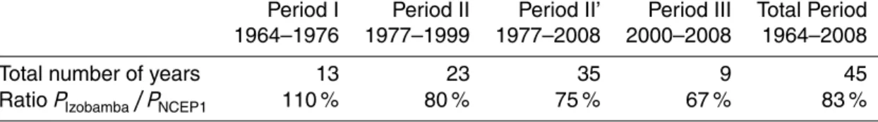
For long term PDD analysis, NCEP1 data from 1964 to 2008 were compared with

20

Izobamba data to obtain long-term daily temperature and precipitation information. The ratio between cumulative daily precipitation from Izobamba and NCEP1 between 1964 and 2008 was 0.83 but varied with time (Table 4). The ratio was close to unity in the 1960s but decreased considerably after 1975 to reach 0.67 between 2000 and 2008. This suggests that the reanalyzed precipitation data should not be directly used for

25

(13)

TCD

8, 2637–2684, 2014

L. Maisincho et al.

Title Page

Tables Figures

◭ ◮

Back Close

Full Screen / Esc

Discussion

P

a

per

|

Discus

sion

P

a

per

|

Discussion

P

a

per

|

Discussion

P

a

per

|

was corrected, multiplied by the ratio observed in the 1960s (i.e. 1.10) to retrieve the mean precipitation observed at Izobamba. Then, in the same way as for Izobamba precipitation, these data were additionally corrected by a factor of 0.74 to fit the mean field precipitation at Antizana, as explained above.

3.3.2 Glaciological data

5

In this study we used (Table 3):

1. daily melting amounts for 43 days in 2002–2003 obtained using “melting boxes” described in Favier et al. (2004a). A melting box, similar to those described by Wagnon et al. (1999), is a cylindrical box with a 50 cm radius with a gridded bot-tom, which is filled with snow or ice. This box is placed inside a slightly bigger

10

box in which snow or ice melt collects. The melting box is inserted in the snow or ice to reproduce the surface condition of the glacier as faithfully as possible. The weight of these boxes is measured at regular intervals (with a precision of ±1 g). In the study by Favier et al. (2004a), special care was taken to discard all measurements disturbed by liquid precipitation in the boxes.

15

2. The annual Antizana 15α vertical mass balance profiles (VBP) were computed from field measurements and the ELA from 2000 to 2008 (Basantes Serranoet al., 2014). All details regarding the glaciological measurements and methods are de-scribed in Francou et al. (2004).

3. The Antizana 15α glacier-wide annual mass balance (Ba) of from 2000 to 2008

20

computed from field measurements. Here we present data from Basantes Ser-rano et al. (2014), in which the glacier-wide annual mass balance of the Antizana Glacier 15α computed using the glaciological method was recalculated using a new, more accurate delimitation of the glacier; and adjusted with the geodetic method which uses digital elevation models (DEM) made from aerial photographs

25

(14)

TCD

8, 2637–2684, 2014

L. Maisincho et al.

Title Page

Tables Figures

◭ ◮

Back Close

Full Screen / Esc

Discussion

P

a

per

|

Discus

sion

P

a

per

|

Discussion

P

a

per

|

Discussion

P

a

per

|

surface. Basantes Serrano et al. (2014) showed that on Antizana Glacier 15α the cumulative mass balance computed using the glaciological method differed signif-icantly from the one computed using the geodetic method, so that the adjustment by the geodetic method was indispensable to accurately quantify the annual mass balance. The discrepancy between the two methods has several causes, but the

5

main cause is that inaccurate interpolation of the mass balance values is done over the glacier surface area where no measurements are conducted. This rep-resents more than 60 % of the glacier surface area. This is the case between the accumulation (at about 5300 m a.s.l.) obtained from the lowest elevation pit or snow core and from the highest ablation stake (at about 5000–5050 m a.s.l.).

10

As a consequence, the shape of the VBP there is conjectural. This inaccurate estimation of accumulation results in significant underestimation of the total mass balance (which can reach 60 % for some years). The reader should refer to Bas-antes Serrano et al. (2014) for more details. Hereafter, the adjusted specific mass balance is referred to as the measured specific mass balance.

15

4. The modeled VBP values were spatially interpolated to assess the modeled glacier-wide annual mass balance. Interpolation required incorporating the point mass balance over the entire surface area of the glacier. For this task, we as-sumed that the point mass balances were representative of the mean glacier mass balance over specific surface areas of the glacier. We assumed the same

20

area as the one used for field glacier-wide mass balance computations. Hence, the annually updated hypsometry and glacier surface area of the Antizana Glacier 15αcomputed by Basantes Serrano et al. (2014) using the 1997 and 2009 digital elevation models established using aerial photogrammetry and the annual topo-graphical measurements of the glacier tongue outline were used to compute the

25

glacier-wide annual mass balance with the PDD model.

(15)

TCD

8, 2637–2684, 2014

L. Maisincho et al.

Title Page

Tables Figures

◭ ◮

Back Close

Full Screen / Esc

Discussion

P

a

per

|

Discus

sion

P

a

per

|

Discussion

P

a

per

|

Discussion

P

a

per

|

the glacier during field trips between 2004 and 2008 were used. The daily snow-line elevation was also estimated from photographs obtained with a low resolu-tion automatic camera (Fujifilm FinePix 1400) installed on the frontal moraine at 4785 m a.s.l. These photographs were taken from the location point called “Photo” in Fig. 1, and were georeferenced (Corripio, 2004). The georeference and contrast

5

between ice and snow on the pixels of each photographs enabled us to retrieve the daily snowline for a period of five years (2004 to 2008). A total of 712 good quality daily photographs allowed us to almost continuously monitor the snowline elevation over time. The elevation was obtained with an accuracy of±10 m.

4 Results and discussion

10

4.1 Estimating degree-day factors for snow and ice

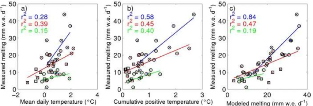
The mean daily temperature and the cumulative hourly positive temperature values at daily time step were first compared with melting amounts from field measurements ob-tained with melting boxes placed close to the AWS in 2002–2003. The surface state of the contents of the boxes was observed and recorded during field campaigns to

15

allow separation into different classes: snow or ice. We also observed that clean and dirty ice should be separated because much more melting took place in the case of dirty ice, despite the minor differences in incoming fluxes and in mean measured tem-perature. As a consequence, we created three classes: snow, clean ice and dirty ice (Fig. 2). A comparison between albedo values measured at the AWS and the initial

20

classification between the different surface states suggests that dirty and clean ice can be separated assuming an albedo threshold of 0.35 (Fig. 2). It was more difficult to detect a threshold between snow and clean ice, as clean ice albedo may occasionally exceed that of snow. This is mainly because of the patchy distribution of snow on the surface of the glacier during the period when the “melting box” experiment was

con-25

(16)

TCD

8, 2637–2684, 2014

L. Maisincho et al.

Title Page

Tables Figures

◭ ◮

Back Close

Full Screen / Esc

Discussion

P

a

per

|

Discus

sion

P

a

per

|

Discussion

P

a

per

|

Discussion

P

a

per

|

snow may remain below the pyranometer, whereas the surface of the melting box was free of snow. Thus, albedo measurements were not always representative of the sur-face state of the melting box. A typical albedo threshold between snow and clean ice surfaces of 0.6 was consequently assumed. However, despite this classification, mean daily temperature was poorly correlated with the measured melting rates (Fig. 3a).

5

Data suggest that melting often starts even when the mean daily air temperature is negative. Indeed, over the 43 days of direct field observations with significant melting amount, we observed that the mean daily air temperature was negative for nine days. For example, a daily melting of 3.8 mm.w.e. d−1on 31 July 2002 was observed when the mean daily air temperature was−1.3◦C. This situation has already been observed

10

in Greenland (Van den Broeke et al., 2010), where a−5◦C threshold was necessary to remove modeling biases caused by the occurrence of short periods of melting when significant nocturnal refreezing occurred. Indeed, these periods were characterized by negative mean daily air temperatures due in particular to unbalanced longwave budgets at night, but also by major incoming shortwave radiation leading to diurnal melting.

15

The correlations were more significant when we assumed the cumulative hourly pos-itive temperature values computed at a daily time step (Fig. 3b). Surprisingly, the latter correlations were similar to those obtained between measured melting amounts and estimated values using a surface energy balance approach for clean ice (Fig. 3c). The PDD approach performed even better for snow surfaces. This may be due to the

oc-20

casional differences in the surface state below the pyranometer and on the surface of the melting boxes. Indeed, the air temperature was not impacted by small scale varia-tions in albedo, which on the other hand, had a major impact on surface energy balance computations. This was particularly true in the case of patchy snow surfaces. Moreover, measurement uncertainties for melting and surface energy balance may partly explain

25

this paradox. We assumed that the agreement between measured melting amount and cumulative hourly positive temperature values was sufficient to calibrate the degree-day factor values for snow, clean ice and dirty ice. This led to three degree-degree-day factors for snow (Fsnow=4.9 mm.w.e. K

−1

d−1), clean ice (Fclean_ice=6.5 mm.w.e. K

−1

(17)

TCD

8, 2637–2684, 2014

L. Maisincho et al.

Title Page

Tables Figures

◭ ◮

Back Close

Full Screen / Esc

Discussion

P

a

per

|

Discus

sion

P

a

per

|

Discussion

P

a

per

|

Discussion

P

a

per

|

dirty ice (Fdirty_ice=12.7 mm.w.e. K

−1

d−1). Managing the distinction between clean and dirty ice is not easy for PDD modeling. For this reason, we included data from dirty and clean ice melting boxes in the same category. Even if this yields lower corre-lations between cumulative degree-day and melting, a degree-day factor for ice was computed,Fice=9.8 mm.w.e. K

−1

d−1. TheF values were similar to those obtained for

5

other glaciers (Radic and Hock, 2011), even though assuming dirty ice conditions led to a slightly higher coefficient for Antizana 15 Glacier than for other glaciers. These values initially reflect a correlation between melting and temperature at a 30 min time scale, but we assumed the values are also valid at a daily time scale.

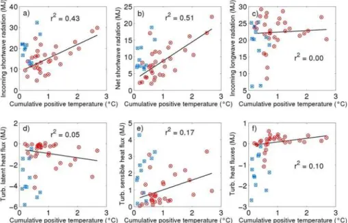
The cumulative hourly positive temperature values were compared to the mean local

10

energy fluxes to check whether a correlation between melting and temperature could be explained by the local processes. We first analyzed data on days with direct melt measurements (Fig. 4) because on these days, sublimation was calibrated with lysime-ters, and we consequently had more confidence in our computed values of turbulent heat fluxes. Except during Period 1 when high winds and low moisture induced high

15

turbulent heat fluxes, the cumulative hourly positive temperature values were signifi-cantly correlated with incident shortwave radiation and with the net shortwave radiation (S) (Fig. 4a and b). Indeed, due to significant local air mixing, air temperature was closely correlated with surface temperature (when<0◦C) and to the duration of diur-nal melting, which mainly depended on the net energy stored at the surface. Thus, if

20

we refer to the period from 14 March 2002 to 31 March 2003, the relationship between air temperature and melting makes sense, because the net shortwave radiation was by far the most important variable involved in melting processes (r=0.78,n=376) and in surface temperature. The correlations with other fluxes were not significant (Fig. 4c–f). Turbulent heat fluxes (LE+H) were generally close to zero because LE and H were

25

(18)

TCD

8, 2637–2684, 2014

L. Maisincho et al.

Title Page

Tables Figures

◭ ◮

Back Close

Full Screen / Esc

Discussion

P

a

per

|

Discus

sion

P

a

per

|

Discussion

P

a

per

|

Discussion

P

a

per

|

estimating ablation in Period 1. Nevertheless, the discrepancy was limited because the high sublimation amounts were also associated with lower temperatures in Period 1 than during the rest of the year. Thus, computing melting with cumulative hourly pos-itive temperature values led to low melting values during Period 1, in agreement with the decrease in melting caused by the highly negative latent heat flux during this period

5

(Favier et al., 2004a).

4.2 Validation of degree-day factors over the 2002–2003 period

To test the accuracy of the degree-day factors derived in Sect. 4.1, we computed daily melt over one annual cycle (2002–2003) using the degree-day model, and compared them with melting results of the SEB computation (Favier et al., 2004a). The melting

10

resulting from SEB computation is hereafter referred to as SEB melting.

We first analyzed whether the mean daily temperature values could be used to run the PDD model instead of the cumulative hourly positive temperature values. At an annual timescale, without separating snow and ice surface states, the correlations be-tween the two variables (daily temperature and cumulative hourly temperature at daily

15

scale) and daily SEB melting were similar and quite low (r =0.58 in both cases, for 376 days). Because the interest of PDD modeling is being able to estimate the impact of past and future climate on glaciers, and since historical hourly temperature data are not available, we analyzed whether mean daily temperature would allow the daily melting to be modeled.

20

We separated days according to their surface state (snow, clean ice and dirty ice). We then multiplied the mean daily temperature by the corresponding F value from Sect. 4.1. The resulting melting values are hereafter referred to asT/melting. We first assumed that snow was present at the AWSG1station when the albedo was higher than

0.6 and that ice was dirty when the albedo was lower than 0.35, while clean ice

condi-25

(19)

TCD

8, 2637–2684, 2014

L. Maisincho et al.

Title Page

Tables Figures

◭ ◮

Back Close

Full Screen / Esc

Discussion

P

a

per

|

Discus

sion

P

a

per

|

Discussion

P

a

per

|

Discussion

P

a

per

|

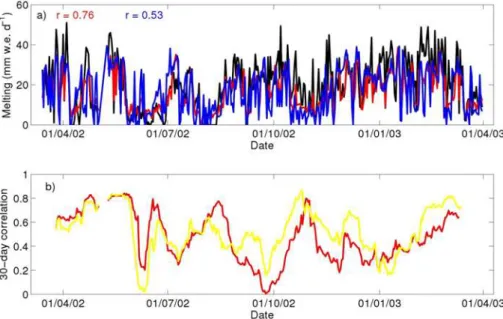
ice (albedo=0.45, instead of 0.35) led to a higher correlation between the T/melting and the SEB melting (r=0.76, n=376 days, Fig. 5a). Nevertheless, as mentioned in Sect. 4.1., in order to obtain the same melting amounts during the 2002–2003 pe-riod we had to assume that melting began when the daily temperature was negative. Indeed, observations showed that melting was frequently significant when the mean

5

daily temperature was still negative (Fig. 6). And in fact, this had a major impact on

T/melting values, because melting amounts were underestimated if we considered that melting began only when mean daily air temperature was 0◦C. Calibration of this threshold was performed to retrieve the magnitude of SEB melting amounts with the PDD model, which yielded a threshold value of−1.9◦C. A frequency analysis showed

10

that 3 % of the melting events in 2002–2003 happened at a mean daily temperature be-low−1.9◦C (Fig. 6), meaning this optimized value was justified. Hereafter, a threshold of−1.9◦C was assumed for PDD modeling. With this assumption, we observed that the mean daily temperature yielded high correlations with SEB melting, and that the annual melting cycle was accurately reproduced (Fig. 5a). The marked difference in

15

melting amounts between Period 1 and Period 2 was reproduced, demonstrating that taking sublimation, or more generally turbulent heat fluxes, into account is not a major limitation to the use of PDD models in Ecuador.

To understand this significant correlation, we compared theT/melting with the di_ff er-ent energy fluxes recorded at the AWSG1. A significant correlation was found between

20

the T/melting and the net shortwave radiation S (r=0.71, n=376 days). A moving correlation between S and theT/melting over 30 days showed variations over the an-nual cycle. This correlation generally reached 0.8 when temperature presented signif-icant variations over a period of one month. However, the correlation decreased when there were no variations in temperature over a long period. This was the case in the

25

(20)

TCD

8, 2637–2684, 2014

L. Maisincho et al.

Title Page

Tables Figures

◭ ◮

Back Close

Full Screen / Esc

Discussion

P

a

per

|

Discus

sion

P

a

per

|

Discussion

P

a

per

|

Discussion

P

a

per

|

temperature values used in the study by Sicart et al. (2008), because albedo is a key driver of melting (Favier et al., 2004a).

Ultimately, and importantly, we decided that melting conditions can be distinguished according to two surface classes only, i.e. ice and snow. We thus assumed that melting was computed with Fice when albedo was lower than 0.45 and with a higher Fsnow

5

than this value. This produced similar correlations to our previous analysis (r =0.75,

n=376) and the mean annual melting value was still respected (only 12 % lower than the melting computed with the SEB). As a consequence, correctly distinguishing ice and snow and obtaining the corresponding degree-day factors allowed us to retrieve variations in melting even when temperature only presented low magnitude variations.

10

4.3 PDD modeling of the period 2000–2008

4.3.1 Modeling of the distributed surface mass balance

Degree-day factors for ice (Fice) and for snow (Fsnow), and the threshold temperature

from Sects. 4.1 and 4.2 were assumed to enable melting modeling using the mean daily temperature and precipitation recorded from 2000 to 2008 at 4900 m a.s.l. in the

15

vicinity of Antizana Glacier 15α. The PDD model was applied at every elevation range, assuming that sublimation is negligible, and compared to the surface mass balance (SMB) measurements made on the glacier. Indeed, sublimation represents about 4 % of total ablation at 4900 m a.s.l. (Favier et al., 2004). This rate may increase with ele-vation as melting amounts decrease, but its variations with eleele-vation are not correctly

20

known.

Overall, the modeled VBP agreed with the observed VBP (Fig. 7). The point mass balance was correctly modeled at the summit and in the ablation zone. Nevertheless, we noted several discrepancies in our modeling results. Differences were observed for the VBP in 2002, whose trend was poorly reproduced above 4850 m a.s.l., and in

25

(21)

TCD

8, 2637–2684, 2014

L. Maisincho et al.

Title Page

Tables Figures

◭ ◮

Back Close

Full Screen / Esc

Discussion

P

a

per

|

Discus

sion

P

a

per

|

Discussion

P

a

per

|

Discussion

P

a

per

|

was generally correctly assessed, even though the model sometimes suggested more accumulation than observed (in 2001 and 2002 for instance) which might result from both measurement uncertainty and the inability of the model to exactly reproduce pro-cesses at high elevations. Moreover, the lowest elevation accumulation data in 2008 was doubtful, leading to highly inaccurate surface mass balance interpolation and to

5

incorrect assessment of the ELA.

However, the largest discrepancy was the incorrect reproduction of point mass be-tween 5000 and 5300 m a.s.l. This discrepancy was very likely due to the interpolation of SMB values between the ablation measured at the highest elevation and accumula-tion measured at the lowest elevaaccumula-tion (Basantes Serrano et al., 2014). Modeling

con-10

firmed this point (Fig. 7) and the SMB profiles in this area are unlikely to vary linearly. We observed that the discrepancies between modeled and measured point mass bal-ance were lower when the measurements were made close to the ELA (i.e. in 2001). Conversely, the discrepancy was high when the linear interpolation between the lowest elevation snow pit and the highest elevation ablation stake strongly deviated from the

15

SMB profiles due to lack of field measurements close to the ELA.

On the other hand, with the assumedFicevalue, the modeled ablation in the ablation

zone was generally slightly overestimated, except in 2002 and 2003. Albedo measure-ments made on the ablation zones of glaciers 15 and 12 between 1999 and 2008 (Glacier 12 is also called Los Crespos Glacier, e.g., Cauvy et al., 2013) showed that

20

albedo was particularly low during the 2002–2003 cycle, suggesting that the ice was frequently dirty (Fig. 8). In particular, albedo values in 2002 and 2003 were frequently below 0.3 (missing data between 17 December 2001 and 14 March 2002 are not ac-counted for in Fig. 8, which would have increased the number of occurrences in 2002). This situation occurred less frequently during the other years of study, suggesting that

25

the ice was more often clean. The PDD model was thus applied again, but this time using the clean ice degree-day factor (Fclean_ice=6.5 mm.w.e. K

−1

(22)

TCD

8, 2637–2684, 2014

L. Maisincho et al.

Title Page

Tables Figures

◭ ◮

Back Close

Full Screen / Esc

Discussion

P

a

per

|

Discus

sion

P

a

per

|

Discussion

P

a

per

|

Discussion

P

a

per

|

Bauder, 2009) reflecting variations in albedo (since degree-day factors for ice differ depending on the surface state). Again, melt variability is mainly determined by varia-tions in incoming short wave radiation and melt-albedo feedback, whereas other SEB terms most closely linked with temperature (L↓, LE and H) are not significantly cor-related with ablation. Hence, using a model that includes incident shortwave radiation

5

may partly reduce the discrepancy observed in the case of low albedo (e.g. Pellicciotti et al., 2005). However, obtaining accurate forecasts or reconstructions for radiation at a regional scale requires a more complex approach than for temperature, and the application of such a model would require additional downscaling steps, which would reduce the interest of the PDD approach compared to SEB computations.

10

Next, our computed glacier-wide annual mass balances were integrated over the whole glacier area and compared to the specific mass balance from Antizana Glacier 15α (Basantes Serrano et al., 2014). Assuming Fclean_ice, we observed that the

mod-eled annual mass balance values were close to the measured glacier-wide annual mass balance (r2=0.71,n=9 years). The model produced very similar mean losses

15

to the geodetic mass balance over the entire period (difference of 0.07 m w.e. a−1 over 9 years). This high correlation suggests that temperature and precipitation are the main climatic drivers of glacier mass balance at the regional scale. Moreover, we observed a significant increase in correlations if the degree-day factor Fdirty_ice=

9.8 mm.w.e. K−1d−1 (see previous paragraph) was used in 2002 and 2003 (r2=0.89,

20

n=9 years). However, the slope of the regression line between the modeled and the measured glacier-wide annual mass balances was larger than 1 (Fig. 9). Removing the modeling result for the year 2003 led to a slope value closer to unity (slope=1.12, assumingFclean_ice for every year except 2002). This suggests that the steeper slope of

the regression line mainly resulted from the model’s overestimation of the very

neg-25

(23)

TCD

8, 2637–2684, 2014

L. Maisincho et al.

Title Page

Tables Figures

◭ ◮

Back Close

Full Screen / Esc

Discussion

P

a

per

|

Discus

sion

P

a

per

|

Discussion

P

a

per

|

Discussion

P

a

per

|

the linear interpolation between 5050 and 5300 m a.s.l. resulted in underestimation of the glacier-wide annual mass balance when this area was characterized by high ab-lation (Fig. 7). Figure 7 suggests that the higher the ELA, the larger the uncertainty in the glacier-wide annual mass balance calculated with the glaciological method. The geodetic adjustment is not designed to remove such annual errors, because instead,

5

it distributes corrections of the cumulative errors over each annual value. Even if the uncertainties in the glacier-wide annual mass balance related to the interpolation con-cern lower values than the geodetic adjustment itself, this suggests that the measured glacier-wide annual mass balance is slightly lower than the one shown in Fig. 9, partly explaining why the slope value of the regression line is higher than unity.

10

4.3.2 Modeling the snowline and ELA variations

For further validation of the model, we compared the modeled vs. measured annual ELA, and modeled vs. measured snowline at a shorter time step. The modeled and measured snowline elevations were averaged over 15 days to reduce the impact of the precipitation uncertainty on model results. Indeed, because the tipping bucket rain

15

gauges are not artificially heated, the snow can accumulate inside the funnel and nat-urally melt several hours or even a day after the precipitation occurred. This led to several shifts in the modeled daily snowline time series.

The modeled snowline was in good agreement with the measured snowline (r2=

0.75, n=91, based on 15 day periods, Fig. 10), demonstrating that the model

accu-20

rately represented the altitudinal distribution of accumulation and ablation at a short time scale. This good agreement is partly due to the direct link between solid pre-cipitation and the 0◦C level (e.g., Favier et al., 2004a, b; Francou et al., 2004). The modeled annual ELA was also in good agreement with the measured ELA (r2=0.77,

n=9 years), a direct consequence of the good agreement between the modeled and

25

(24)

TCD

8, 2637–2684, 2014

L. Maisincho et al.

Title Page

Tables Figures

◭ ◮

Back Close

Full Screen / Esc

Discussion

P

a

per

|

Discus

sion

P

a

per

|

Discussion

P

a

per

|

Discussion

P

a

per

|

4.4 Using the PDD model with data from remote stations or reanalysis data

The glacier-wide annual mass balances were computed using Fsnow=

4.9 mm.w.e. K−1d−1) and Fclean_ice=6.5 mm.w.e. K

−1

d−1, for the 2000–2008 pe-riod using data from a remote meteorological station located at Izobamba. Because data were measured at distinct elevations and under slightly different climatic settings,

5

a correction was applied on Izobamba temperature and precipitation data to obtain similar mean values to those at 4900 m a.s.l. during the 2000–2008 period.

First, the model was applied using temperature data from Izobamba, which were corrected with a lapse rate of−6.0◦C km m−1 to retrieve similar mean annual values as those observed on Antizana over the period 2000–2008. The experiment revealed

10

a significant correlation between the observed and the computed glacier-wide annual mass balances (r2=0.72, n=9 years, Fig. 9b), suggesting that temperature varia-tions at Izobamba meteorological station were representative of the regional climate responsible for the glacier retreat observed over the last decade. In the second step, we applied the model to both temperature and precipitation at Izobamba. To reduce

15

the bias in precipitation amounts caused by regional features and differences in eleva-tion, Izobamba data were multiplied by a factor of 0.74 to fit the precipitation observed on Antizana Glacier 15α. This modeling resulted in a slightly lower correlation with measured data (r2=0.63, n=9 years, Fig. 9b), suggesting that the occurrence and amounts of precipitation are very important for the computation of the glacier mass

20

balance at an annual scale.

Next, we applied the PDD model on NCEP1 data assuming that precipitation should be multiplied by a factor 0.5 (as mentioned in Sect. 3.3.1), whereas the reanalyzed temperature at 570 hPa (4900 m a.s.l.) was linearly interpolated from data at 600 and 500 hPa. The results of this experiment were in good agreement with measured values

25

(25)

TCD

8, 2637–2684, 2014

L. Maisincho et al.

Title Page

Tables Figures

◭ ◮

Back Close

Full Screen / Esc

Discussion

P

a

per

|

Discus

sion

P

a

per

|

Discussion

P

a

per

|

Discussion

P

a

per

|

Finally, given the close relationship between temperature and melting, we wanted to explain the occurrence of the almost equilibrated mass balances in Ecuador between 1956 and 1976 as suggested by studies on Antizana glacier (e.g., Francou et al., 2000; Basantes Serrano et al., 2014) and on the neighboring Cotopaxi Volcano (Jordan et al., 2005). To this end, we analyzed the long term temperatures measured in the field and

5

temperatures from NCEP1 reanalysis and those recorded at Quito meteorological sta-tion. Both temperature time-series were in agreement in suggesting that a slight cooling occurred during the 1960s and at the beginning of the 1970s (Fig. 11), whereas atmo-spheric warming has been recorded since the end of the 1970s (Vuille and Bradley, 2000; Vuille et al., 2008).

10

Next, PDD modeling was performed to retrieve variations in the ELA. Figure 11a shows that the reanalyzed temperatures were in good agreement with historical tem-peratures recorded at Quito. However, we observed that precipitation data from NCEP1 increased excessively compared with observed precipitation after 1976 and we thus preferred to use measured precipitation at Izobamba instead. We consequently

pro-15

duced a PDD model based on the daily reanalyzed temperature but using Izobamba precipitation for the period between 1964 and 2008. However, we were nevertheless obliged to use reanalyzed precipitation time series before 1964 due to the lack of daily precipitation measurements. To this end, NCEP1 daily precipitation was corrected us-ing the difference in ratio with Izobamba (see Sect. 3.3.1.5). The modeled ELA for the

20

2000–2008 period was in good agreement with the measured ELA (r2=0.86, n=9, data not shown) suggesting that this PDD model was sufficiently accurate to analyze past variations in ELA over time.

Modeling showed good agreement between the modeled ELA (Fig. 11) and the above mentioned glacier advance in the 1960s and the 1970s (Rabatel et al., 2013)

25

(26)

TCD

8, 2637–2684, 2014

L. Maisincho et al.

Title Page

Tables Figures

◭ ◮

Back Close

Full Screen / Esc

Discussion

P

a

per

|

Discus

sion

P

a

per

|

Discussion

P

a

per

|

Discussion

P

a

per

|

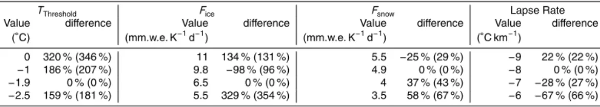
5 PDD sensitivity

A sensitivity test of the computed specific mass balance was performed on the main model parameters: (Table 5) the temperature threshold, the degree-day factors for ice and snow, and the temperature lapse rate with elevation. This test showed that the model was particularly sensitive to the temperature threshold because this parameter

5

directly increased both snow and ice melting. Nevertheless, the value was quite robust as it was obtained from different consistent approaches. The degree-day factor for ice was also crucial because it controlled melting in the lower part of the glacier, i.e. where melting was very high. The correlation coefficient between the melting boxes and tem-perature were slightly more significant for ice, suggesting that this factor was correctly

10

assessed. But we also demonstrated that this parameter can change depending on the surface state. It may thus be important to better constrain this parameter in the future. Here, we tried to better constrain this parameter with a regression analysis between ablation obtained from stakes positioned in the field and positive degree day sums at a monthly scale. Unfortunately, due to systematic alternation of snow and rainfall events

15

at the surface of the lower part of the glacier, it was not possible to separate ice and snow surfaces, or to extract accumulation from point mass balance measurements at the stake locations. Concerning the degree-day factor for snow, this parameter had less impact on the final model because it mainly acted on melting in the highest part of the glacier, where the temperature was usually negative. Nevertheless, its value would be

20

crucial in cold snowy years (during La Niña events), i.e., when conditions are favorable for glacier mass gains. Finally, the lapse rate was accurately obtained from measure-ments in the field, and had no marked impact on the final mass balance values.

6 Conclusion

The good agreement between temperature and glacier melting and mass balance

25