! " # $%& '(&&)&&& *+ ,- . /
* / +
-# ! " /
# (' 0$&&)10& , / -# . /
2 2 +
3 + 45
' 6%&)&&& - . /
!
"#
This paper studies the linear feedback control strategies for nonlinear systems. Asymptotic stability of the closed-loop nonlinear system is guaranteed by means of a Lyapunov function, which can clearly be seen to be the solution of the Hamilton-Jacobi-Bellman equation thus guaranteeing both stability and optimality. The formulated Theorem expresses explicitly the form of minimized functional and gives the sufficient conditions that allow using the linear feedback control for nonlinear system. The numerical simulations the Duffing oscillator and the nonlinear automotive active suspension system are provided to show the effectiveness of this method.
Keywords: optimal control, nonlinear system, duffing oscillator, active suspension system,
chaotic attractor
Introduction
1Since the first publications (Krasovskii, 1959), (Kalman and
Beltram, 1960) and (Letov, 1961), in the early 1960s, the Lyapunov function techniques have been used in studying optimal control problems.
It is well known that the nonlinear optimal control problem can be reduced to the Hamilton-Jacobi-Bellman partial differential equation (Bryson and Ho, 1975). There are many difficulties in its solution, in general case. There are, in current literature (see, for example, Bardi and Capuzzo-Dolcetta, 1997), several methods that may be used in obtaining a numerical solution of the Hamilton-Jacobi-Bellman partial differential equation. In particular case, the quadratic Lyapunov function is a solution of the Hamilton-Jacobi-Bellman equation for the linear system with the quadratic functional. In recent years, the idea that a Lyapunov function for the nonlinear system can be an analytical solution of the Hamilton-Jacobi-Bellman equation has become popular.
In Bernstein (1993) a unified framework for continuous-time nonlinear-nonquadratic problems was presented in constructive manner. The results of Bernstein (1993) are based on the fact that steady-state solution of the Hamilton-Jacobi-Bellman equation is a Lyapunov function for the nonlinear system thus guaranteeing both stability and optimality.
In Haddad et al. (1998) the framework developed in Bernstein (1993) was extended to the problem of optimal nonlinear robust control. There are no systematic techniques for obtaining the Lyapunov functions for general nonlinear systems in this case, but this approach can be applied to systems for which the Lyapunov functions can be found.
In Rafikov and Balthazar (2004) the nonquadratic nonlinear Lyapunov function was proposed to resolve the optimal nonlinear control design problem for the Rössler system.
This paper studies the linear feedback control strategies for nonlinear systems.
Paper accepted July, 2008. Technical Editor: Marcelo Amorim Savi.
Asymptotic stability of the closed-loop nonlinear system is guaranteed by means of a Lyapunov function, which can clearly be seen to be the analytical solution of the Hamilton-Jacobi-Bellman equation thus guaranteeing both stability and optimality. The formulated Theorem expresses explicitly the form of minimized functional and gives the sufficient conditions that allow using the linear feedback control for nonlinear system.
Nomenclature
A = bounded matrix (nxn) B = constant matrix (nxm)
s
b = damping force, N/m/s
l s
b = damping force linear, N/m/s
nl s
b = damping force nonlinear, N/m/s
y s
b = damping force symmetric, N/m/s g = vector (nx1)
G = matrix (nxn)
s
k = suspension stiffness, N/m
l s
k = suspension stiffness linear, N/m
nl s
k = suspension stiffness nonlinear, N/m
t
k = tyre stiffness, N/m
s
m = sprung mass, kg
u
m = unsprung mass, kg P = Riccati equation (nxn) Q = matrix (nxn)
V = Lyapunov function t = time, s
x
= displacement of the flexible beam, m x = velocity of the flexible beam, m/s x = acceleration of the flexible beam, m/s2 y = state vectorc
c
z = vertical velocity of the sprung mass , m/s
c
z = vertical acceleration of the sprung mass , m/s2
w
z = vertical displacement of the unsprung mass , m
w
z = vertical velocity of the unsprung mass , m/s
w
z = vertical acceleration of the unsprung mass , m/s2
r
z = disturbance caused by road irregularities, m
Greek Symbols
α = stiffness parameter, N/m
ζ = viscous damping coefficient, N/m/s γ = amplitude external input, m ω = angular frequency, rad/s Γ = neighborhood
Subscripts
s sprung u unsprung t tyre
Superscripts
l linear nl nonlinear y symmetric
Linear Design for Nonlinear System We consider the nonlinear controlled system
Bu y g y t A
y= () + ( )+ ,y(0)=y0 (1)
where y∈ℜn is a state vector, A(t)∈ℜn×n is a bounded matrix,
which elements are time dependent, B∈ℜn×m is a constant matrix,
m
u∈ℜ is a control vector, and g(y)∈ℜn is a vector, which elements are continuous nonlinear functions, g(0)=0.
We remark that the choice of A(t) is not unique, and this influences the performance of the resultant controller.
Assume that:
y y G y
g( )= ( ) (2)
where G(y)∈ℜn×n is a bounded matrix, which elements depend on y. If we assumed (2), the dynamic system (1) has the following form:
Bu y y G y t A
y= () + ( ) + (3)
Next, we present an important result, concerning a control law that guarantees stability for a nonlinear system and minimizes a nonquadratic performance funcional.
Theorem 1. If there exist matrices Q(t) and R(t), positive definite, being Q symmetric, such that the matrix:
) ( ) ( ) ( ) ( ) ( ) , ( ~
y G t P t P y G t Q t y
Q = − T − (4)
is positive definite for the bounded matrix G , then the linear feedback control:
y t P B R
u=− −1 T () (5)
is optimal, in order to transfer the non-linear system (3) from an initial to final state:
0 ) (tf =
y (6)
minimizing the functional:
dt u R u y Q y
J T T
tf
) ~
(
0
+
=
∫
(7)where the symmetric matrix P(t) is evaluated through the solution of the matrix Ricatti differential equation:
0
1 + =
− +
+PA A P PBR−B P Q
P T T (8)
satisfying the final condition:
0 ) (tf =
P (9)
In addition, with the feedback control (5), there exists a
neighborhood Γ0⊂Γ, Γ⊂ℜn, of the origin such that if y0∈Γ0,
the solution y(t)=0, t>0, of the controlled system (3) is locally
asymptotically stable, and Jmin =y0TP(0)y0.
Finally, if Γ=ℜn then the solution y(t)=0, t>0, of the controlled system (3) is globally asymptotically stable.
Proof. Lets consider the linear feedback control (5) with matrix P determined by equation (8) which transfers the nonlinear system (3) from an initial to a final state (6), minimizing the functional (7) where the matrix Q~ need to be determined.
According to the Dynamic Programming rules one knows that if the minimum of functional (7) exists and if V is a smooth function of the initial conditions, then it satisfies the Hamilton-Jacobi-Bellman equation (Bryson and Ho, 1975):
0 ~
min =
+ +y Qy u Ru dt
dV T T
u
(10)
Considering a function:
y t P y
V = T () (11)
where P(t)is a symmetric matrix positive definite and it satisfies the differential Riccati equation (8).
Note that the derivative of the function V, evaluated in the optimal trajectory with control given by (5) is:
y P y y t P y y t P y
V = T () + T () + T =[yTAT(t)+yTGT(y)− +
+ −yTP(t)B(R−1)TBT]P(t)y yTP(t)y
] ) ( )
( ) ( [ )
(t At y G y y BR 1B Pt y P
yT + − − T
+
Then, substituting V in the Hamilton-Jacobi-Bellman equation (10) one obtains:
P y G P B PBR PA P A P
Then:
) ( ) ( ) ( ) ( ) ( ~
y G t P t P y G t Q
Q= − T − .
Note, that for positive definite matrices Q~ and R, the derivative of the function (11) is given by V=−yTQ~y−uTRu, and, it is negative
definite. Then, the function (11) is Lyapunov function, and the controlled system (3) is locally asymptotically stable. Integrating the derivative of the Lyapunov function (11) given by
u R u y Q y
V=− T~ − T along the optimal trajectory, we obtain
. ) 0
( 0
0 min y P y
J = T
Finally, if Γ=ℜn, global asymptotic stability follows as a direct consequence of the radial unboundedness condition for the Lyapunov function (11) V(y)→∞ as y →∞.
We remark that according to the optimal control theory of linear systems with quadratic functional (Anderson and Moor, 1990) the solution of the nonlinear differential Riccati equation (8) is positive definite and symmetric matrix P>0 for all R>0 e Q≥0 given, one can conclude the Theorem proof.
If the time interval is infinite and A, B, Q and R are matrix with constant elements, the positive defined matrix P is the solution of the nonlinear, matrix algebraic Riccati equation
0
1 + =
−
+A P PBR−B P Q
PA T T . (12)
Linear Design for Duffing Oscilator
We will apply the proposed method to the Duffing oscillator that is one of the paradigms of nonlinear dynamics.
The Duffing oscillator with the control law U(t) is described by the following nonlinear differential equation:
) ( cos 2
3 x t U t
x x
x=−α − − ζ +γ ω + (13)
where α is the stiffness parameter, ζ >0 is the viscous damping coefficient, γ and ω are the amplitude and frequency of the external input, respectively.
For α<0, the Duffing oscillator without control can be interpreted as a model of a periodically forced steel beam which is deflected toward the two magnets, as shown in Fig. 1.
Figure 1. Mechanical interpretation of Duffing oscillator.
Let the desired trajectory be a function ~x(t). Then the desired regimen is described by the following equation:
u t x
x x
x ~ ~ 2 ~ cos ~
~=−α − 3− ζ +γ ω + (14)
where u~ is a control function which maintains the Duffing oscillator in the desired trajectory. If the function ~x(t) is a solution of equation (13) without the control term then u~=0.
Subtracting (14) from (13) and defining:
− − =
x x
x x
y ~
~
(15)
we will obtain the following system:
u x x y y y y
y y
+ + + − − − = =
3 3 1 2 1 2
2 1
~ ) ~ ( 2ζ
α (16)
where u=U−u~ is feedback control.
So the equation (3) in this case has the following form:
u y
y x x x y x y
y y
y y
+
− + − + − +
+
− − =
1 0 0
0 ~ ~ ) ~ ( ) ~ (
0 2 1 0
2 1 2 1
2 1
2 1
2 1
ζ α
(17)
Let the desired trajectory be a periodic orbit:
t t
x 2cos sin
~= + (18)
and the parameters α =−1, ζ=0.125, γ=1 and ω=1.
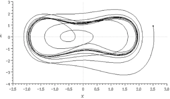
These are exactly the same desired trajectory and parameters as reported by Sinha et al. (2000). For these parameters, the system (14) without control possesses a chaotic attractor, shown in Fig. 2.
Figure 2. Phase portrait of uncontrolled Duffing oscillator.
Choosing
=
1 0
0 1
Q andR=
[ ]
1, then one obtains
=
1771 . 2 4142 . 2
4142 . 2 6825 . 3
P by solving the Riccati equation (12) using the
= − −
= ( ) ( )
~
y PG P y G Q
Q T −
−
−
22 12
12 11 1
0 0
) ~ , ( 0
p p
p p x y
Q ϕ
−
−
0 ) ~ , (
0 0
1 22 12
12 11
x y p
p p p
ϕ
+
=
0 2 ) ~ , (
22 22 12
1 p
p p x y
Q ϕ
where ϕ(y1,~x)=(y1+~x)2+(y1+x~)~x +~x2.
Note that the function ϕ(y1,~x) has its minimum value
2 min ~
4 3 x =
ϕ in y x~
2 3
1=− because ϕ′=2y1+3x~1 ϕ′′=2>0, then
2
1 ~
4 3 ) ~ , (y x ≥ x
ϕ and, admitting 3≥ ~x ≥1, one can evaluate Q~ as:
=
+ ≥
+ ≥
0 2
4 3 0
2 ~ 4 3 ~
22 22 12
22 22 12 2
p p p Q p
p p x Q
Q
1 632825 . 1
632825 . 1 6213 . 4
positive definite.
Finally, we can conclude that the optimal function u has the following form:
2 1 2.1771
4142 .
2 y y
u=− − . (19)
The phase portrait behavior of the controlled Duffing oscillator is presented in Fig. 3.
Figure 3. Phase portrait of controlled Duffing oscillator.
Linear Design for Nonlinear Automotive Active Suspension System
Consider a quarter vehicle model that captures the fundamental features of the suspension design of the vehicle. A typical quarter-car suspension system is shown in Fig. 4.
Figure 4. Typical quarter-car suspension system.
In this figure, ms represents the sprung mass, which corresponds
to 1/4 of the body mass, and the unsprung mass mu represents the
wheel at one corner. The parameters kt; ks; bs are the tyre stiffness,
the suspension stiffness, and the damping rate of the suspension, respectively. The control signal u is generated by the actuator, zc
and zw denote the vertical displacement of the sprung mass and the unsprung mass, respectively. The disturbance w is caused by road irregularities.
Several methods to solve the active suspension problem have been proposed. The most part of these research contributions are based on linear time-invariant suspension models for control design.
Thompson (1976) was the first to explore the use of optimal control techniques to design an active law.
Active suspension design, using linear parameter varying control, was considered by Gaspar et al. (2003).
The real physical systems always include nonlinear components which must be taken into consideration. The suspension force generated by the hydraulic actuator is inherently nonlinear; the dynamic characteristics of suspension components, i.e., dampings and springs, have nonlinear properties.
To resolve the active suspension problem for nonlinear system in this work we will apply the linear feedback control design above considered.
The equations of motion of the vehicle active suspension system are (Gaspar et al., 2003):
(
)
(
)
u z z k
z z b z z b z z k z z k z m
u z z b z z b z z k z z k z m
r w t
c w y s c w l s c w nl s c w l s w u
c w y s c w l s c w nl s c w l s c s
+ − −
− − + − − − − − − =
− − − − + − + − =
) (
) ( ) (
) ( ) (
3 3
(20)
Here, parts of the nonlinear suspension damping bs are bsl, bsnl
and bsy.
The bsl coefficient affects the damping force linearly, and bsy describes the symmetric behavior of the characteristics. Parts of the
nonlinear suspension stiffness ks are a linear coefficient ksl and a
nonlinear oneksnl.
0 ~ , ~ , 0 ~ , ~ = = = = w w c
c w z z w z
z (21)
Noting that the desired trajectory is a solution of the system (20) without control and defining:
[
]
Tw w c
c w z z w z
z
y= − − (22)
we will obtain the following equation in form of (1):
Bu y g y A
y= + ( )+ (23)
where: − + − − − = u l s u t l s u l s u l s s l s s l s s l s s l s m b m k k m b m k m b m k m b m k A ) ( 1 0 0 0 0 0 1 0 , − = u s m m B 1 0 1 0 − + − − − − − = 2 4 3 1 3 2 4 3 1 3 ) ( 0 ) ( 0 ) ( y y m b y y m k y y m b y y m k y g u y s u nl s s y s s nl s
. (24)
Considering:
y
g
g
g
g
g
g
g
g
y
y
G
y
g
=
=
44 43 42 41 24 23 22 210
0
0
0
0
0
0
0
)
(
)
(
where:);
,
(
;
)
(
4 2 44 42 24 22 2 1 3 43 41 23 21y
y
m
b
g
g
g
g
y
y
m
k
g
g
g
g
s y s s nl sδ
=
=
−
=
−
=
−
−
=
=
−
=
−
=
≠ − − = − = 0 if ) ( 0 if 0 ) , ( 2 4 2 4 2 4 4 2 y y y y sign y y y y δwe present the equation (23) in form (3).
The proposed linear feedback design procedure has been applied to the quarter car suspension with the following values of the parameters (Gaspar et al., 2003): ms=290kg, mu=40kg,
m N
ksl=23500 / , ksnl=2350000N/m, kt=190000N/m,
s m N
bsl=700 / / e bsy=400N/m/s.
For these parameters the matrix A has the following form:
− − − − = 5 . 17 5 . 5337 5 . 17 5 . 587 1 0 0 0 414 . 2 034 . 81 414 . 2 035 . 81 0 0 1 0 A . Choosing = 100 0 0 0 0 100 0 0 0 0 100 0 0 0 0 100
Q , R=[0.00001], then one
obtains: − − − − − − = 0187 . 1 5918 . 2 2583 . 0 5828 . 1 5918 . 2 1816 . 6411 1348 . 110 2601 . 584 2583 . 0 1348 . 110 2626 . 10 0896 . 12 5828 . 1 2601 . 584 0896 . 12 4481 . 687 P
by solving the Riccati Eq. (12).
Finally, we can conclude that the optimal function u has the following form:
4 3
2
1 2892.7037 31494.7352 2457.7889
5054 .
211 y y y y
u= + − − (25)
For numerical simulations the disturbances of the initial conditions y1=−0.05 m and y3=−0.05m were considered. Fig. 5
and 6 show y1 and y3 variations without and with control (25), respectively.
Figure 5. Comparison of the time traces of the variable of the controlled system (23) and the same system without control.
It is difficult to analyze the matrix Q~ analytically in this case.
Fig. 7 shows the positive function L(t)=yTQ~y, calculated in optimal trajectory.
Figure 7. Time trace of the positive function.
Conclusions
The optimal linear feedback control strategies for nonlinear systems were proposed. Asymptotic stability of the closed-loop nonlinear system is guaranteed by means of a Lyapunov function which can clearly be seen to be the solution of the Hamilton-Jacobi-Bellman equation thus guaranteeing both stability and optimality.
The formulated Theorem expresses explicitly the form of minimized functional and gives the sufficient conditions that allow using the linear feedback control for nonlinear system.
The numerical simulations for the Duffing oscillator and the nonlinear automotive active suspension system are provided to show the effectiveness of this method.
Finally we note that the proposed method can be applied to a large class of nonlinear and chaotic systems.
Acknowledgements
The work was partially supported by the Brazilian Government agencies CNPq and FAPESP.
References
Anderson, B.D.O. and Moor, J.B., 1990, “Optimal Control: Linear Quadratic Methods”, Prentice-Hall, NY.
Bardi, M. and Capuzzo-Dolcetta, I., 1997, “Optimal Control and Viscosity Solutions of Hamilton-Jacobi-Bellman Equations”, Birkhäuser, Boston.
Bernstein, D.S., 1993, “Nonquadratic cost and nonlinear feedback control”, Int. J. Robust Nonlinear Contr. 3, pp. 211-229.
Bryson, JR., A.E. and Ho, Y. C., 1975, “Applied optimal control: Optimization, Estimation, and Control”. Hemisphere Publ. Corp., Washington D.C..
Gaspar, P., Sazaszi, I. and Bokor, J., 2003, “Active suspension design using linear parameter varying control”, International Journal of Vehicle Autonomous Systems, Vol. 1, No. 2, pp. 206-221.
Haddad, W.M., Chellaboina, V. S. and Fausz, J.L., 1998, “Robust nonlinear feedback control for uncertain linear systems with nonquadratic performance criteria”, Systems Control Lett., 33, pp. 327-338.
Krasovskii, N. N., 1959, “On the theory of optimum control”, Appl. Math. Mech., vol. 23, pp. 899-919.
Kalman, R.E. and Bertram, J.E., 1960, “Control system analysis and design via the second method of Lyapunov”, Journal of Basis Engineering, vol. 82, pp. 371-393.
Letov, A.M., 1961, “The analytical design of control systems”,
Automation and Remote Control, 22, pp. 363-372.
Rafikov, M. and Balthazar, J. M., 2004, “On an optimal control design for Rössler system”, Phys. Lett., A 333, pp. 241-245.
Sinha, S.C., Henrichs, J.T. and Ravindra, B.A., 2000, “A general approach in the design of active controllers for nonlinear systems exhibiting chaos”, Int. J. Biff. Chaos, 10 (1), pp. 165-178.