J. Braz. Soc. Mech. Sci. & Eng. vol.27 número2

S. I. S. de Souza

H. A. Vielmo

Departamento de Engenharia Mecânica Rua Sarmento Leite, 425 90050-170 Porto Alegre, RS. Brazil vielmoh@mecanica.ufrgs.br

Numerical Analysis of Water Melting

and Solidification in the Interior of

Tubes

Latent energy storage systems find applications in many engineering fields, including industrial refrigeration plants, air conditioning installations, recovery of heat in industrial processes, etc. To tackle the design of such systems, it is necessary to have correlations to account for the heat transfer during the melting and solidification of the phase change material (PCM). This work describes and analyzes the results obtained from the numerical simulation of pure water melting and solidification in the interior of tubes, which are typically present in ice banks of air conditioning systems. The shown results consider natural convection, accounting for the inversion in the water density. In the melting process, the considered initial conditions followed the classical Stefan and Neumann approach. The presented simulation results include the evolution of the phase change interface, and of the temperature, density and streamlines fields. Correlations for the Nusselt number and for the melted material volume as functions of time have been proposed.

Keywords: Phase change, melting and solidification, ice banks, finite volumes, polar geometry

Introduction

The increasing energy demand and the requirements for an environmentally sustained development have been major motivating factors for the implementation of more efficient means of energy conservation. In addition to conservation, the rational use of energy has been the focus of many studies, so that the processes are more efficient and less expensive, reducing waste, preserving the environment and the nonrenewable energy sources, and avoiding unnecessary expenses. In this sense, the employment of thermal energy storage has the objective of making the energy consume more rational. This storage is performed in three basic, distinct ways: sensible heat, latent heat and chemical. The systems that operate with sensible heat require high temperature differences with respect to the environmental, as well as a storage substance with large mass. This leads to some disadvantages, to mention the need of large spaces to accommodate the system and thick, expensive thermal insulation. The storage systems that use the latent heat present a superior amount of volumetric capacity, besides requiring smaller temperature differences with respect to the environment, which decreases the thermal insulation expenses.1

According to the “ASHRAE Applications (1995)”, the use of thermal storage systems may be an economically attractive approach for heating or cooling loads when they are of short time duration and occur cyclically; when there is an incompatibility with the available energy source, or its supply is limited; when the energy costs are time-dependent; and when economical incentives are provided for the use of load-shifting equipment.

In the refrigeration field, ice banks have been employed as an energy storage solution to reduce the electrical power required during the hours of peaks in the demand, shifting the consume curve to a more favorable situation. It must be noted that in many countries, the cost of industrial electricity is time dependent during the day, having higher values in the periods of high demand. It can be also mentioned the contractual demand, resulting into a fine to the user in case the energy consumption is exceeded. Aiming at economical feasibility, it has been increasingly attempted to develop systems that employ the storage of latent heat, despite its disadvantages. Among those, it can be mentioned the inherent

Paper accepted May, 2005. Technical Editor: Clóvis R. Maliska.

irreversibilities due to heat transfer, the decrease in the efficiency of the thermodynamic cycle due to the decrease in the evaporation temperature in the air-conditioning installations, the increase in the physical space that is necessary to accommodate the ice bank, and uncertainties in the evaluation of the heat transfer between the PCM and the system working fluid.

Water in the solid phase has been employed as the storage substance due to its properties and characteristics: high melting latent heat (334 kJ/kg), melting temperature of 0°C at the atmospheric pressure, accessibility, low cost, no pollutant effects, and chemical stability. As the most important disadvantage characteristic, it can be pointed the supercooling phenomenon (a metastable equilibrium) during the solidification, “Chen and Lee (1998)”. The ice bank consists of thermally insulated tanks that are inserted into a refrigeration loop. In some systems, the ice is formed on the outside of the tubes. In such systems, a limit must be impose to the ice thickness formed on the piping, since if it exceeds a given value there will be a decrease in the heat transfer during the discharge process, caused by the ice thickness and the flow obstruction. Examples of works that investigated the phase change occurring in the outside of the tubes are “Ho and Chen (1986)”, “Zhang and Faghri (1996)”, “Abugderah and Ismail (2000)”, “Stampa et al. (2002)”.

Nomenclature

A = area, m2 B = body force, m/s2 c = specific heat, J/kg

E = coefficient of the proposed function for the Kirchhoff temperature, coefficient of the Nusselt number correlation Fo = Fourier number , 2

0

t r

α

g = gravitational field, m/s2

h = enthalpy, J/kg; convection heat transfer coefficient, W/(m2K)

k = thermal conductivity, W/(mK) L = representative grid size

L = average thickness of the liquid ring, m m = mass, kg

Nu = Nusselt number,

(

)

0

0ln s 0 adm r r r r r ∂T ∂r ₌ p = pressure, N/m²

q = heat transfer rate, W

r = radial coordinate, mesh relation, radius, m Rac = Rayleigh number, *b_3

ref g T T L

η − αν

Ste = Stefan number,

(

)

p p

c T −T λ

T = temperature, °C, K t = time, s

u = tangential velocity, m/s V = volume, m³

v = radial velocity, m/s

Greek Symbols

α = thermal diffusivity, m2_/s

β = thermal expansion coefficient, 1/K Φ = generic variable

η = 9.297173x10-6, °C-b

λ = melting and solidification latent heat, J/kg

µ = dynamic viscosity, Ns/m2 ν = kinematic viscosity, m2/s θ = angular coordinate, rad ρ = density, kg/m3

Subscripts

c = relative to convection

conv relative to convective process f = relative to melting

H = relative to hydrostatic component ini = relative to initial

L = relative to liquid max = relative to maximum mist = relative to mixture p = relative to constant pressure r = relative to radial direction ref = relative to reference s = relative to solid S = relative to solid w = relative to wall

0 = relative to tube wall or to initial

θ = relative to angular direction, angular position

Superscripts

* = melting point

b = 1.894816, constant to “Eq. 31”

Physical Model and Boundary Conditions

The focus of this work is a latent “cold storage” modulus, which consists of a bank of tubes containing pure water inside, subjected to

a crossed external flow. In the present approach only one tube is considered through a symmetric, two-dimensional model, since such tubes are typically subjected to small temperature variations along its length.

The boundary conditions are now established in order to facilitate the physical model comprehension. For the thermal problem the first-kind boundary conditions are adopted, “Eq (1)”, both for the melting and solidification, as seen in “Fig.1”.

In the melting process Tw>T *

, and in the solidification process Tw<T*, where Tw is the tube wall temperature and T* is the melting temperature (in this work T*=0 °C).

For the hydrodynamic problem, the slip and non-permeability boundary conditions are imposed on the surfaces of the tube and of the solid PCM,

0

0 S

u= =v → r=r and r=r (2) where u and v are, respectively, the angular and radial velocities,

and r0 and rs are the radius of the tube and of the PCM, as seen in “Fig. 1”. The initial condition adopted for the thermal problem during the melting is dependent on the approach that is applied. In the so called Stefan problem,

Figure 1. Computation domain.

( )

, 0

T rθ =T → t= (3)

while in the Neumann problem,

( )

T rθ =T → t= (4)

In the solidification the initial boundary condition, for the thermal problem, is:

( )

T rθ =T → t= (5)

where T(r,θ) is the temperature inside the tube, Tini is the initial temperature and the subscripts S and L stand for the solid and liquid regions, t is time, r and θ are respectively the radial and angular coordinates.

For the hydrodynamic problem, the initial conditions for the melting and solidification are:

0 0

u= =v → t= (6)

Governing Equations

The heat transfer from or to the encapsulated fluid originates the thermal gradients, which in turn cause the existence of gradients in the density in the interior of the fluid domain. Therefore, thermal convection may be present due to the fluid flow caused by buoyancy. For the solution of such a problem, it is necessary the knowledge of the velocity, temperature, density and pressure fields, which characterizes the coupling of the hydrodynamic and thermal problems. The equations that govern the phenomenon for the considered geometry are present below in radial coordinates. The continuity equation is given by:

( )

( )

1 1

0

r v u

t r r r

ρ ρ

ρ

θ

∂ ∂

∂ + + =

∂ ∂ ∂ (7)

where ρ is the density and t is de time. The momentum equations in the r and θ directions are:

( )

( )

( )

( )

2 ₂

2

2 2 2

1 1

1 1 2

r

r v

v uv u p

t r r r r r

rv v u

B

r r r r r

ρ

ρ ρ ρ

θ

µ _{θ θ} ρ

⎛∂ ∂ ∂ ⎞ ∂

⎜ + + + ⎟=− +

⎜ ∂ ∂ ∂ ⎟ ∂

⎝ ⎠

⎡∂ ⎛ ∂ ⎞ ∂ ∂ ⎤

+ ⎢_⎢∂ ⎜ _∂ ⎟+ _∂ + _∂ ⎥_⎥+

⎝ ⎠

⎣ ⎦

(8)

( )

(

)

( )

( )

2

2

2 2 2

1 1 1

1 1 2

u

u r vu uv p

t r r r r r

ru u v

B

r r r r r θ

ρ

ρ ρ ρ

θ θ

µ _{θ θ} ρ

⎛∂ ∂ ∂ ⎞ ∂

⎜ + + + ⎟= − +

⎜ ∂ ∂ ∂ ⎟ ∂

⎝ ⎠

⎡∂⎛ ∂ ⎞ ∂ ∂ ⎤

+ ⎢_⎢∂ ⎜ _∂ ⎟+ _∂ + _∂ ⎥_⎥+

⎝ ⎠

⎣ ⎦

(9)

in which p is the pressure, and Br and Bθ are the radial and angular components of the gravitational field acceleration g. The dynamic

viscosity is represented by µ. The Boussinesq approximation is

adopted for the buoyancy terms in the liquid phase. The references for the temperature and density are taken from the melting point:

Tref=T* and ρref=ρ*. From the Maxwell thermodynamic relations, one can set the state equation that relates the density to temperature and pressure for a given substance:

( , )T p

ρ ρ= (10)

For small variation in the density, it is acceptable to expand the above function in the vicinity of a point of reference by means of the Taylor series to give:

(

)

(

)

ref ref ref

p T

T T p p

T p

ρ ρ

ρ ρ≅ +_⎜⎛∂ ⎞_⎟ − +⎛_⎜∂ ⎞_⎟ − +

∂ ∂

⎝ ⎠ ⎝ ⎠ (11)

which is valid for liquids. Using now the definition of the thermal expansion coefficient β, “Eq. (11)” becomes:

(

)

1

ref Tref T

ρ ρ≅ ⎡_⎣ +β − ⎤_⎦ (12)

inserting “Eq. (12)” into “Eq. (8)” and “Eq. (9)” results:

( )

( )

( )

( )

(

)

2 ₂

2

* *

2 2 2

1 1

1 2

H

v

v uv u p rv

t r r r r r r r

v u

g cos T T

r r

ρ

ρ ρ ρ _µ

θ

ρ β θ

θ θ

⎛∂ ∂ ∂ ⎞ ∂ ⎡∂⎛ ∂ ⎞

⎜ + + + ⎟=− + ⎢ ⎜ ⎟+

⎜ ∂ ∂ ∂ ⎟ ∂ _{⎢ ⎝⎣}∂ ∂ _⎠

⎝ ⎠

⎤

∂ ∂

+ _∂ + _⎥+ −

∂ ⎦

(13)

( ) ( )

( )

( )

(

)

2

2

* *

2 2 2

1 1 1

1 2

H

u

u vu uv p ru

t r r r r r r r

u v

g sen T T

r r

ρ

ρ ρ ρ _µ

θ θ

ρ β θ

θ θ

⎛∂ ∂ ∂ ⎞ ∂ ⎡∂⎛ ∂ ⎞

⎜ + + + ⎟=− + ⎢ ⎜ ⎟+

⎜ ∂ ∂ ∂ ⎟ ∂ _{⎢ ⎝⎣}∂ ∂ _⎠

⎝ ⎠

⎤

∂ ∂

+ _∂ + _⎥− −

∂ ⎦

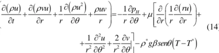
(14)

where pH is the pressure that incorporates the hydrostatic component. Since the density of the water is not a linear function of the temperature, “Fig. 2”. The behavior of the volumetric expansion coefficient, with respect to the temperature, was based on the expression of “Vasseur et al. (1983)”, for the water density, resulting in the following expression:

7 2 5 5

1.9364 10x T 1.7507012 10x T 6.59759847 10x

β_{= −} − ₊ − ₋ − ₍₁₅₎

Figure 2. Behavior of the water density with respect to the temperature.

In problems of phase change, the domain can be divided into three distinct regions: solid, liquid and interface, where each region has its own characteristics. For the pure substances, the temperature is constant in the liquid-solid interface, and so it does not provide any information on the evolution of the process. To overcome this difficulty, it is considered the energy equation in the enthalpy form. Applying the model proposed by “Cao et al. (1989)”, in which it is employed the concept of the Kirchhoff Temperature, described and applied in “Vielmo (1993)”, results:

( )

( )

( )

( )

( )

2

2 2 2 2

1 1 1 ( )

1 ( ) 1 1

h r vh uh h h

r

t r r r r r r

S h S h

h h r

r r r r r

ρ ρ ρ

θ

θ θ

∂ ₊ ∂ ₊ ∂ ₌ ⎛∂ ∂Ε⎛ ⎞⎞₊

⎜ ⎟

⎜ ⎟

∂ ∂ ∂ ⎝∂⎝ ∂ ⎠⎠

⎛ ⎛ ∂ ⎞⎞ ∂

∂ Ε ∂

+ _∂ + ⎜_⎜∂⎜ _∂ ⎟⎟_⎟+ _∂

⎝ ⎠

⎝ ⎠

(16)

where h is the specific enthalpy. The remaining terms are described below:

( )

_{( )}

( )

( )

_{( )}

_{( )}

( ) 0 0 ( )

0 ( ) 0 0 ( )

( ) ( )

S p S

L L

p _L p _L

k

h S h h Solid phase

c

h S h h Interface

k k

h S h h Liquid phase

c c

λ

λ _λ

Ε = = → ≤ →

Ε = = → < < →

Ε = = − → ≥ →

(17)

Numerical Methodology

For the integration of the governing equations, the finite volumes method is applied, as described in “Patankar (1980)” and “Maliska (2004)”.

In the equation, the diffusion coefficient depends whether the considered region is the liquid, interface or solid. The system of equations resulting from the integration of the differential equations is solved by the TDMA scheme, with a block correction. The adopted interpolation function is the Power-Law, and the coupling between the pressure and velocity fields is based on the SIMPLEC algorithm. A computational mesh formed by 40x40 volumes was employed after grid independence tests were performed. The velocities are stored in the interfaces of the control volumes. In most of the solutions, relaxation factor of 0.8 for all the variables proved to be adequate to deal with the non-linearities of the problem.

Values in the order of 10-8 were used for convergence criteria,

applied to relative error of each variable between two consecutive iterations, as well as to the residual masses in each control volume. In order to obtain stable, implicit transient solutions, the time steps were varied and chosen so that the enthalpy, in the liquid domain, changed about 200 J/kg each time step (no control volumes submitted to the phase change). When there were control volumes close to the phase change region (the biggest period of time), the time steps were reduced to values that caused variation in the enthalpy in the range of approximately 10 J/kg in the liquid.

Validation of the Proposed Methodology

For the validation, the results obtained in this work were compared to the numerical and experimental results presented in “Rieger and Beer (1986)”, “Fig. 3”. The solid is kept fixed in the center of the tube. Figure 4 presents the solution obtained in this work for the same situation considered in the aforementioned work. As seen, there exists an excellent agreement between the two solutions.

Figure 3. On the top the experimental results of “Rieger and Beer (1986)”, obtained for Tw = 6

o

C, r0 = 0.03 m, SteFo = 0.053. On the bottom their

numerical solution for, Tw = 6

o

C, r0 = 0.032 m, SteFo = 0.059.

Figure 4. Solution obtained in the present work. The streamlines and the isotherms are presented on the left and right sides, respectively, for

Tw=6

o

C, SteFo=0.059, r0=0.032 m.

For verification of the independence of the solutions with respect to the discretization, it was applied the Grid Convergence Index (GCI), according to “Roache (1998)”, and the usual procedure for estimation and reporting of discretization error in CFD applications. The melting was simulated using the Stefan approach for the initial condition Tini,S=0 °C, for the boundary condition

Tw=10 °C and for a tube with a diameter r0=0.032 m. The following equations were initially applied to evaluate the apparent order p of

the employed method:

( )

1

1 N

i i

L A

N =

⎡ ⎤

=_⎢ ∆ _⎥

⎣

∑

coarse fine

L r

L

= (19)

( )

3 2

2 1

f f ln

f f p

ln r − −

= (20)

where L is the representative grid size, the ∆Ai is the area of the i th volume, and N is the total number of volumes used. The f terms are the solutions, and the subscripts 1, 2 and 3 refer from the more refined to the less refined mesh. The three different meshes tested have 40×40, 120×120 and 360×360 control volumes. Such an approach was necessary to allow geometrical agreement between the evaluation points. The temporal agreement was also observed. The enthalpy was the variable used for the inspection of the apparent order p of the method, since this property is the key variable in the problem. The obtained results are presented in “Tab. 1”.

Such evaluations were carried out for three angular positions in the tube, and in each position three locations were chosen along the radius. The angles of the positions are referred to with respect to the “Fig. 1”. These positions were chosen in such a way to cover the upper, intermediary and lower regions of the tube.

For the evaluation of the relative error, ε, and of the GCI, “Eq’s. (21) and (22)” were employed considering the apparent order p of local approximation, “Eq. (20)”:

2 1

1

f f f −

ε = (21)

1 25 1

p

GCI . r

ε

Table 1. Results of the relative error and the GCI for the initial condition Tini,S=0°C, boundary condition Tw=10°C, and r0 = 0.032 m. Employed meshes of 40×40, 120×120 and 360×360, and r=1.73.

Position Enthalpy h (J/kg) f2=f40

f1=f120

f2=f40

f1=f360

f2=f120

f1=f360

Time (s) θ r (m) Grid

40x40

Grid

120x120

Grid

360x360

Apparent Order p

ε (%)

GCI

(%) (%) ε

GCI

(%) (%) ε

GCI

(%)

0.026 342055.8 344052.8 345020.03 1.32 0.58 0.68 0.86 1.01 0.28 0.33

0.0292 365261.8 365862.3 365954.8 3.4 0.16 0.037 0.19 0.04 0.025 0.006

24.75°

0.0316 374208.5 374187.9 374182.9 2.99 0.006 0.002 0.007 0.002 0.001 0.0003

0.0268 343134.8 341944.2 342088.3 3.85 0.35 0.007 0.31 0.05 0.042 0.007

0.0292 357059.1 356843.2 356637.5 0.08 0.06 1.45 0.12 3.0 0.057 1.47

92.25°

0.316 372748.7 372767.9 372737.3 -0.84 0.005 -0.028 0.003 -0.01 0.008 -0.03

0.026 337294.5 336438.4 336042.5 1.41 0.254 0.273 0.372 0.4 0.118 0.13

0.0292 354062.5 354562.98 354421.2 3.92 0.141 0.0.023 0.157 0.026 0.016 0.003

1250

155.25°

0.0316 372178.6 372316.9 3723340.0 3.26 0.037 0.009 0.043 0.011 0.0062 0.0015

As seen in the “Tab. (1)”, the maximum relative error, ε,

reached values lesser than 1 % in the comparison of the results

obtained for the meshes 40×40 and 360×360. The CGI presents a

maximum error of approximately 1.5 % for the meshes 40×40 and

120×120. One can be state, based on the results presented in “Tab. (1)”, that the employed grid of 40×40 control volumes proved to be adequate for the analysis presented in this work. Also it is possible to observe the appearance of a negative value for the apparent order

p, indicating an oscillatory convergence in that position (close to the

center of the tube). In this position low values for the relative errors also occur. In rare situations these variations, when close to zero, are indicative that the exact solution was reached. Anyway, it does not represent unsatisfactory calculations, or parameter to invalidate the results.

In all the obtained solution, for the different meshes, it was not registered any variation in the pattern of the variables fields. The verification of the presence or not of multiple solutions was investigated through alterations in the directions of the TDMA scheme. As observed, changing the directions in all directions did not cause any modification in the solutions.

Results and Discussion

The Nusselt Number

It is first necessary to define an expression for the Nusselt number in the melting of the PCM encapsulated in the interior of the tube, and for that matter it was adopted the enclosure treatment. For the geometry considered in this work, the solution of the steady-state, one-dimensional diffusion equation, with no source term, provides the below temperature profile:

*

0

0

( ) ln

ln

w

w s

T T r

T r T

r r r

⎛ ⎞ −

= _{⎛ ⎞ ⎝ ⎠}⎜ ⎟+ ⎜ ⎟ ⎝ ⎠

(23)

The heat transfer by diffusion, qr , in a given position r is given by:

( )

0

0 0

ln 2

ln ln

w w

r w

s s

d T T r T T

q k A r T k

dr r r r

r r

π

⎡ ⎤

⎢ _{− ⎛ ⎞} ⎥ ₋

⎢ ⎥

= − _{⎢ ⎜ ⎟}+ _⎥= −

⎛ ⎞ _{⎝ ⎠} ⎛ ⎞

⎢ ⎜ ⎟ ⎥ ⎜ ⎟

⎢ ⎝ ⎠ ⎥ ⎝ ⎠

⎣ ⎦

(24)

The convective heat transfer qconv is written using the general formulation below:

(

)

0

( )

conv c w

q = −A r h T −T (25)

where hc is the heat transfer coefficient. In a situation where the PCM is partially liquid and solid, but before the convection has started, the heat rate across r0 is therefore transferred by diffusion to

the liquid up to the phase change boundary. In this situation, it can be written:

( )

(

)

0

*

*

0 0

0

( )

2 2

ln

w

c w

r r s

T r T T

k A r k r h T T

r r

r

π π

=

∂ −

− = − = − −

∂ ⎛ ⎞

⎜ ⎟ ⎝ ⎠

(26)

The Nusselt number is then defined for this problem as the relation qconv/qr0. For the situation of pure diffusion:

0 0

0

ln 1

conv c s r

q h r

Nu r

q k r

⎛ ⎞

= = ⎜ ⎟=

⎝ ⎠ (27)

( )

( )

(

)

(

)

0

0 0

*

0

0 *

0

( , )

ln

( , ) ln

conv r r

r w

s

s r r w

T r k A r

q r

Nu

q T T

k A r r r

r

r T r r

r r

T T

θ θ

θ

θ

=

= ∂

−

∂

= = =

− −

⎛ ⎞ ⎜ ⎟ ⎝ ⎠

⎛ ⎞ ∂

= _{− ∂} ⎜ ⎟

⎝ ⎠

(28)

Inserting the dimensionless temperature profile, Tadm, into “Eq. (28)”, the local Nusselt number becomes:

0 0

0

ln s adm

r r

r T Nu r

r r

θ

= ⎛ ⎞ ∂

= _{⎜ ⎟ ∂}

⎝ ⎠ (29)

The Nusselt number, thus defined, represents a relation between the existing convective heat rate and the heat rate that would exist in case the process were purely diffusive. All the previous equations provide results for a control volume in a given angular position θ, and time t. In engineering, the main interest usually is the average behavior of the phenomenon. Therefore, it is interesting to determine the average behavior of the Nusselt number, which is done in the following way:

( )

( )

0

0 0

1 1

2

A r

Nu Nu dA r Nu d

A r

π

θ _π θ θ

=

_∫

_∫

Results for the Melting Process

Next, it is presented the solutions for the wall boundary conditions of Tw=4 oC and Tw=8 oC, applied to a tube with radius

r0=0.032 m, and starting at the initial condition in the solid of

Tini,S=T*=0 oC. The thermal resistance imposed by the tube wall was neglected. Since the phenomenon is transient, solutions were collected at various instants t for the two wall boundary conditions. The streamlines in the liquid region are plotted in the same graphs of the density. This allows a better understanding of the

phenomenon associated with the inversion in the density,based on

the observation of the local Nusselt number, “Eq. (29)”, and of the average Nusselt number, “Eq. (30)”.

Firstly, “Fig. 5” shows the solutions for Tw=4 oC. In the figure, the behavior of the local Nusselt number as a function of the angular position is presented. In the initial instants, as for t=100 s, it can be noted that the phenomenon is purely diffusive, indicating an equality between the heat rates, as described in “Eq. (27)”.

For t=3000 s, there are variation of the Nusselt number with the angle. It can be observed the beginning of the convective effects through a small increase on the Nusselt number for the angular positions in the upper region, 0°<θ<100°. For the lower region, 100°<θ<180°, there is a decrease in the value of the Nusselt number. The maximum temperature that the liquid reached in this simulation was 4 °C, while the minimum was 0 °C. The portion of liquid with the highest temperature will assume the highest density. Due to the gravitational field action, the fluid with the lowest density and temperature will be concentrated in the upper positions, and so intensifying the heat rate in that region. The fluid with the highest temperature and density will occupy the lower positions of the tube, leading to a decrease in the heat rate from the wall to the fluid. As a result, the Nusselt number presents values lower than the unity. This decrease occurs due to the assumptions taken for the derivation of “Eq. (26)”, in which it was considered that the heat rate that penetrates in the boundary by diffusion is mostly transported by

advection in the interior of the tube. In “Fig. 6”, it can be observed the evolution of the phase change boundary as well as the behavior of the process parameters, temperature and density, which validate the aforementioned explanations. The temperature evolution demonstrates the concentration of liquid with higher temperatures in the lower regions of the domain. The aforementioned characteristics of the process intensify with the time evolution; that is, the Nusselt number increases in the upper positions and decreases in the lower positions.

1 1 1 1 1 1 1 1 1 1 1 1 1 2 2 2 2 2 2 2 ₂

2 2 2 2 2 3

3 3

3 3

3

3 ₃ 3 3

3 3 3 4

4 4

4 4

4 4

4 4

4 4

4 4 5

5 5

5

5

5

5

5

5 5

5 5 ₅ 6

6

6

6 6

6

6

6 6

6

6 6 6

θ

Nu

50 100 150

0 1 2 3 4 5 6 7

t=100 s t=3000 s t=5000 s t=7000 s t=12000 s t=18000 s

1 2 3 4 5 6

Tw=4°C

Figure 5. Nusselt number behavior as a function of the angle θ and time t for melting withTw=4.

Figure 5 shows the existence of two peaks in the Nusselt number for t=7000 s. For this same instant, “Fig. 6” shows that the vortex structure is complex: two clockwise (negative) vortices, while another vortex spins in the anticlockwise direction. This causes the formation of two locations with peaks in the Nusselt number. This vortex structure is also registered for t=12000 s. In the vortex boundaries, there is a larger mass displacement, which extends from the region close to the solid PCM to the tube wall, originating regions with high thermal gradients, as observed on the left side of the figures, where the temperature field is presented. In initial instants, as for t=5000 s, the first peak in the Nusselt number is due to the formation of a vortex in the upper part of the tube, and a second peak occurs in a intermediary angular position, and is formed by the PCM ring thickness variation in the liquid state. For

t=18000 s, there is another vortex structure. The vortex that spins in

the clockwise direction, a negative vortex, predominates, while a positive vortex, located in the lower region of the domain, does not affect significantly the heat transfer process. In this situation, there is a peak in the Nusselt number in the upper part of the tube, a region where liquid with lower temperature and density is concentrated.

0.00 0.01 0.02 0.03

0.99987 0.99988 0.99989 0.99990 0.99991 0.99992 0.99993 0.99994 0.99995 0.99996 0.99997 0.99998 0.99999 1.00000

ρ/ρ

t=3000 s Temperature °C

-0.03 -0.02 -0.01 0.00

-0.03 -0.02 -0.01 0.00 0.01 0.02 0.03

Vsol=64.83%

Streamlines

0.00 0.01 0.02 0.03

0.99987 0.99988 0.99989 0.99990 0.99991 0.99992 0.99993 0.99994 0.99995 0.99996 0.99997 0.99998 0.99999 1.00000

ρ/ρ

t=7000 s

+

-Vsol=45.15%

-0.03 -0.02 -0.01 0.00

-0.03 -0.02 -0.01 0.00 0.01 0.02 0.03

Temperature Streamlines

0.00 0.01 0.02 0.03

0.99987 0.99988 0.99989 0.99990 0.99991 0.99992 0.99993 0.99994 0.99995 0.99996 0.99997 0.99998 0.99999 1.00000

t=12000 s

ρ/ρ

4°C

Vsol=21.97%

+

--0.03 -0.02 -0.01 0.00

-0.03 -0.02 -0.01 0.00 0.01 0.02 0.03

Temperature Streamline

0.00 0.01 0.02 0.03

0.99987 0.99988 0.99989 0.99990 0.99991 0.99992 0.99993 0.99994 0.99995 0.99996 0.99997 0.99998 0.99999 1.00000

ρ/ρ

t=18000 s

Vliq=97.37%

+

-0.03 -0.02 -0.01 0.00

-0.03 -0.02 -0.01 0.00 0.01 0.02 0.03

Figure 6. On the right, the streamlines (+ means anticlockwise recirculation) are juxtaposed to the density; the temperatures fields for melting with

Tw=4 °C, Tini,S=0 °C, t=3000 s, t=7000 s, t=12000 s, and t=18000 s are shown on the left.

1 1 1 1 1 1 1 1

2 2

2 2

2 2 2 2 2

3 3

3

3 3

3 3

3 3

3

3

4 4

4 4

4 4

4 4

4

4 ₄

4

4

5 5

5 5

5 5

5 5

5 5

5

5

5

6 6

6 6

6 6

6

6 6

6 6

6 6

6

6

6

6

θ

Nu

50 100 150

0 0.5 1 1.5 2 2.5 3 3.5 4 4.5 5 5.5 6 6.5 7 7.5

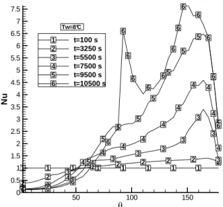
t=100 s t=3250 s t=5500 s t=7500 s t=9500 s t=10500 s

1 2 3 4 5 6

Tw=8°C

Figure 7. Nusselt number behavior as a function of the angle θ and time t, for melting withTw=8

o

C.

The difference between the two solutions can be explained by the inversion in the density for temperatures close to 4 °C. For this wall temperature, there is concentration of liquid with high temperature and lower density in the upper regions. The fluid formed from the melting of solids with lower temperatures also presents a density inferior to the maximum value, and is prone to move to the upper regions. However, as the fluid starts the motion, it mixes with fluids at higher temperature, reaching the temperature of 4 °C, a situation in which the water has the maximum density, and so it moves towards the lower positions of the tube. For the previous situation, Tw=4 °C, there was an inverse behavior, although with the same driving mechanism.

The behaviors of the density and temperature fields for Tw=8 oC can be observed in “Fig. 8”. The simulations indicate that, for situations in which Tw<4 oC, the behaviors are similar to those found for Tw=4 oC, while for Tw>8 oC it is similar to Tw=8 oC. For Tw=6 oC, in the beginning of the process the behavior resembles the situation for Tw=4 oC; after some time, the solution presents an inversion, with a behavior similar to that for Tw=8 oC.

0.00 0.01 0.02 0.03

0.99987 0.99988 0.99989 0.99990 0.99991 0.99992 0.99993 0.99994 0.99995 0.99996 0.99997 0.99998 0.99999 1.00000

ρ/ρ_4°C

t=3000 s Vsol=50,74%

+

+

+

--0.03 -0.02 -0.01 0.00 -0.03

-0.02 -0.01 0.00 0.01 0.02 0.03

0.00 0.01 0.02 0.03

0.99987 0.99988 0.99989 0.99990 0.99991 0.99992 0.99993 0.99994 0.99995 0.99996 0.99997 0.99998 0.99999 1.00000

t=6500 s

ρ/ρ

4°C

Vsol=26,7%

+

+

--0.03 -0.02 -0.01 0.00 -0.03

-0.02 -0.01 0.00 0.01 0.02 0.03

0.00 0.01 0.02 0.03

0.99987 0.99988 0.99989 0.99990 0.99991 0.99992 0.99993 0.99994 0.99995 0.99996 0.99997 0.99998 0.99999 1.00000

t=8500 s

ρ/ρ

4°C

Vsol=13,96%

+

--0.03 -0.02 -0.01 0.00

-0.03 -0.02 -0.01 0.00 0.01 0.02 0.03

0.00 0.01 0.02 0.03

0.99987 0.99988 0.99989 0.99990 0.99991 0.99992 0.99993 0.99994 0.99995 0.99996 0.99997 0.99998 0.99999 1.00000

t=11000 s

ρ/ρ

4°C

Vliq=99,14%

+

+

--0.03 -0.02 -0.01 0.00

-0.03 -0.02 -0.01 0.00 0.01 0.02 0.03

Figure 8. On the right, the streamlines (+means anticlockwise recirculation) are juxtaposed to the density. The temperatures fields for melting with

Tw=8 °C, Tini,S=0 °C , t=3000 s, t=6500 s, t=8500 s, e t=11000 s are shown on the left.

Vf/V0

Nu

(a

v

e

ra

g

e

)

0.2 0.4 0.6 0.8

0 0.2 0.4 0.6 0.8 1 1.2 1.4 1.6 1.8 2 2.2 2.4 2.6

Vf/V0

Nu

(a

v

e

ra

g

e

)

0.2 0.4 0.6 0.8

0 0.5 1 1.5 2 2.5 3 3.5 4 4.5

Tw=4 °C

Tw=8 °C

Figure 9. Average Nusselt number behavior as a function of the relation Vf/V0.

In the search for correlations that enable the evaluation of the heat transfer, and that are not prone to be affected by the “singular” behavior of the water density, it was employed an expression that has been presented in “Sasaguchi et al. (1998)”. Applying it into the dimensionless momentum equations, more specifically in the

buoyancy terms, leads to the following Rayleigh number:

_ *b 3

ref c

g T T L Ra η

αν

−

where η = 9.297173×10-6, L is the average thickness of the liquid ring, b = 1.894816, α is the thremal diffusivity, ν is the kinematic viscosity, and Tref takes the value of Tw in the melting.

This parameter allowed the identification of a pattern behavior of the Nuaverage/Rac ratio, as a function of the melted volume Vf to the initial volume V0 ratio, Vf/V0, and also as a function of Fo, as can be

observed in “Fig. 10”, where logarithm scales were adopted. Such behaviors were approximated by the following relations:

0

f c

V Nu

Log a Log b

Ra V

⎛ ⎞₌ ⎛ ⎞₊

⎜ ⎟ ⎜ ⎟

⎜ ⎟ _{⎝ ⎠}

⎝ ⎠ (32)

( )

0

f

V

Log d Log Fo c V

⎛ ⎞ = +

⎜ ⎟

⎝ ⎠ (33)

where a, b, c and d are the coefficients to be determined. This

allows writing an expression for the Nusselt number in the following way:

1 2

10E E

t c

Nu = Fo Ra (34)

The terms E1 and E2 are defined as:

3 2

1 3 2

531.105 244.60 50.58 1.682 0.1 531.105 259.85 53.95 1.5 0.1

Ste Ste Ste Ste

E

Ste Ste Ste Ste

⎧− + − − → ≤

⎪

= ⎨_{− + − − → >}

⎪⎩ (35)

2

2 2

0.395 0.894 1.6418 0.1

5.2 2.86 1.4924 0.1

Ste Ste Ste

E

Ste Ste Ste

⎧− − − → ≤

⎪

= ⎨ _{− − → >}

⎪⎩ (36)

(

)

L

p w

c T T

Ste

λ

−

= (37)

2 0

t Fo

r

α

= (38)

where the α is the thermal diffusivity.

Based on the behaviors of the presented solutions, it is possible to establish correlations for the melted volume Vf and, consequently, for the average thickness of the melted PCM:

0

10c d

f

V = Fo V (39)

(

)

2

0 0 1 10

d c

L= −r r −Fo (40)

where the terms d and c are obtained according to:

0.2631 0.5304 0.1

1.3044 0.4264 0.1

3.6912 0.4531

d Ste Ste

d Ste Ste

c Ste

= + → ≤

= + → >

= −

(41)

The efficacy of the proposed correlations can be evaluated in “Fig. 11”, where they are compared to the results obtained with the simulation. In the values of the simulations, the percentage variations were added, allowing the visualization of the maximum existing differences between the two results. It can be observed for the Nusselt number that the maximum differences occur at the beginning of the melting process, where the diffusion is the predominant heat transfer mode. In the time periods where the

convection is the dominant mode, the differences between the two solutions decrease. Indeed, in literature, convection correlations with uncertainties as high as 20% occur.

Results for the Melting Process Followed by

Re-solidification

As a consequence of the variable ambient conditions, which cause variations in the thermal load, it is common the partial use of the stored energy in the ice banks along the time. Therefore, simulations considering this situation also must be carried through,

allowing a better knowledge of the heat transfer mechanisms.The

results for the partial melting process followed by resolidification are shown in “Figs. 12 and 13”, considering that the PCM in the solid phase is initially supercooled (Neumann approach), Tini,S=-5

o

C. For t=0 s, the tube wall was exposed to Tw=8

o

C, initiating the melting. After a period of 7760 s, the surface temperature on the

external surface changes to Tw=-5.5

o

C, initiating the resolidification. The behaviors of the enthalpy and density in the domain are also presented. The dashed line represents the enthalpy in the region where the liquid reaches its maximum density, for a temperature of 4 oC. On the left corner on the bottom, the Rayleigh number for the considered instant is presented. Together with the relative density, the streamlines are presented, enabling the visualization of the liquid behavior during the phenomenon evolution. The instants of time for which the simulations were run are presented on the bottom corner.

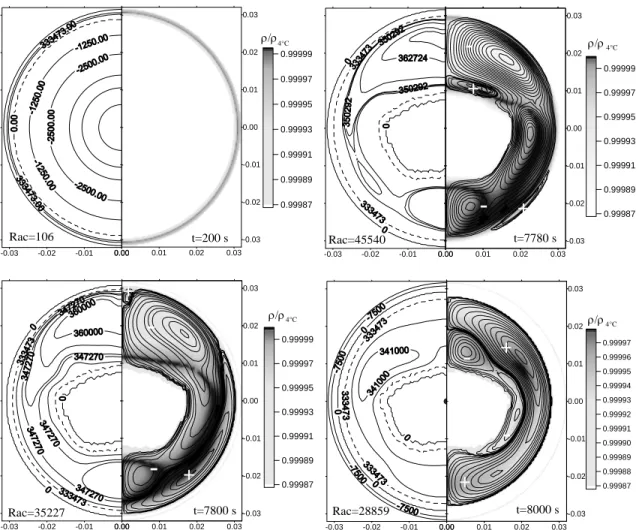
The behavior of the melting process is first shown for the time instant t=200 s. It can be observed that the sensible energy associated with the solid supercooling rapidly disappears, and in this instant diffusion predominates. For t=3000 s, there is no longer traces of sensible energy, and the advection mechanism is already active in the heat transfer. For t=7780 s, the boundary condition is altered so that solidification occurs. One can note a thin layer of solidified material in the external region. The liquid is then confined between the two phase change boundaries. The sensible energy associated with the liquid is released to the two boundaries. This initially reduces the advance of the solidification in the external boundary. In the inner boundary, the melting continues until the thermal equilibrium is reached. Initially, the thickness of the solidified external layer is not uniform, as for when t=7800 s. This occurs due to the fact that it is in the upper region where the liquid with the lowest density and enthalpy level concentrates. This difference is small, being the more intense the larger is the temperature Tw set to cause the melting. In the solidification, the vortices structure changes drastically, as can be observed for the instants t=7780 s, t=7800 s, and t=8000 s. As the solidification advances, the inner liquid and the solid reach thermal equilibrium, as for when t=8750 s. After this, the buoyancy effects become negligible, the velocities associated with the liquid are of such a magnitude that convection stops actuating, so that diffusion predominates again, and the liquid density becomes homogeneous. The inner solid becomes “insulated”, without altering its energetic state until t=10750 s, when the two boundaries meet. From this point ahead, there is heat transfer from the inner solid by diffusion. This can be visualized for time instants later than t=12500 s.

In the solidification, the time and intensity of the natural convection actuation are larger for situation where the initial sensible energy, or equivalently the initial liquid temperature (Tini,L),

is large and when the Tw temperature is low. To evaluate the

1

1

1

1

1

1

1 2

2

2

2

2

2

2 3

3

3

3

3

3

3 4

4

4

4

4

4 5

5

5

5

5

5

5 6

6

6

6

6

6 7

7

7

7

7 8

8

8

8

8

8

Vf/V0

Nu

(a

v

e

ra

g

e

)/

R

a

c

0.2 0.4 0.6 0.8

10-5 10-4 10-3 10-2 10-1 100

Tw=2°C Tw=4°C Tw=6°C Tw=8°C Tw=10°C Tw=12°C Tw=14°C Tw=16°C 1

2 3 4 5 6 7 8

1 1

1 1

1 1

1 1

2 2

2 2

2 2

2 2

3 3

3 3

3 3

3

4 4

4 4

4 4

4

5 5

5 5

5 5

6 6

6 6

6

7 7

7 7

7

8 8

8 8

8

Fo

Vf

/V

0

10-1

100

101 0.1

0.2 0.3 0.4 0.5 0.6 0.7 0.8 0.91

Tw=2°C Tw=4°C Tw=6°C Tw=8°C Tw=10°C Tw=12°C Tw=14°C Tw=16°C 1

2 3 4 5 6 7 8

Figure 10. On the left: behaviors of the Nuaverage/Rac ratio as a function of Vf/V0. On the right: the Vf/V0 ratio as a function of the dimensionless time Fo, for

various wall temperatures Tw

-5.5 -5 -4.5 -4 -3.5 -3 -2.5 -2 -1.5 -1 -0.5

0 0.25 0.5 0.75 1 1.25 1.5 1.75 2 2.25 2.5 Fo

Lo

g

(N

u

/Rac

)

Simulation Correlation

Maxim variation of 15%

Tw=4°C – Ste=0.05

-5.8 -5.3 -4.8 -4.3 -3.8 -3.3 -2.8 -2.3

0 0.15 0.3 0.45 0.6 0.75 0.9 1.05 1.2 1.35

Fo

Log

(N

u

/Ra

c

)

Simulation Correlation

Maxim variation of 10% Tw=8°C – Ste=0.1

0 0.2 0.4 0.6 0.8 1 1.2

0 0.5 1 1.5 2 2.5

Fo

Vf

/V

0

Simulation Correlation

Maxim variation of 12%

Tw=4°C – Ste=0.05

0 0.2 0.4 0.6 0.8 1 1.2

0 0.2 0.4 0.6 0.8 1 1.2 1.4 Fo

Vf/V

0

Simulation Correlation

Maxim variation of 10%

Tw=8°C – Ste=0.1

Figure 11. Comparison between the relations log Nu(average)/Rac and Vf/V0 as functions of Fo obtained from the numerical simulation and from the

Figure 12. Results for the partial melting in the periods t=200 s, t=7780 s, t=7800 s (start of the resolidification), and t=8000 s. On the left and rights sides, respectively, the behaviors of the specific enthalpy and of the density together with the streamlines are presented.

In both situations, it was considered the same physical model, and the same boundary and initial conditions, the difference being solely on the solution method. The first case was dealt considering the solidification process to be purely diffusive; in the other case, the convection mechanism was taken into account.

1

L

L volume mist

p

h dv m

T

c

ρ λ

⎛ ⎞₋

⎜ ⎟

⎜ ⎟

⎝ ⎠

=

∫

The observations show a faster decrease on Tmist in the simulation that took the natural convection into account, and this trend remained the same for the other simulations having different boundary and initial conditions. The difference between the solutions narrowed with the decrease of the liquid sensible energy in the beginning of the process. The time needed for the temperature homogenization in the interior of the liquid domain also decreased for the same reason; the decrease on Tini,L leads to the same effects.

The influences of the natural convection, and of the sensible energy existing in the beginning of the process on the PCM solidification time, can be seen in “Fig. 14” (right side). The results for the two different solidification situations are exposed. For the first and second cases, it was set Tini,L=8 °C and 16 °C. For both

cases, Tw=-5.5 °C and the solutions were obtained for processes with pure diffusion and with natural convection.

Observing the left size of “Fig. 14”, one realizes the proximity between the purely diffusive and natural convection solutions, since the steeper decrease on Tmist when convection is taken into account is not sufficient to cause noticeable differences between them (solidification time). This behavior can be justified by the sensible energy being much smaller than the latent energy (that is, low Stefan numbers). The differences in the values of Tmist /Tini,L between the two observed cases in the left side are consequences of the fluid movement in the convective process, causing a faster homogenization of the temperature in the liquid. The amount of sensible energy in the liquid has small influence on the solidification

speed, for temperatures around Tini,L=8 °C, so that there is a

coincidence between the solutions with natural convection and pure diffusion.

For higher temperatures, as for Tini,L=16 °C, the solidification speed is smaller for the initial instants in the convective process,

Vf/V0>0.6. After the temperature homogenization is reached, for

Vf/V0>0.4, there is an inversion in the solidification speed, and the

convective process becomes faster. In the end of the process, the solidified volume is identical for the two cases, and the time needed for this to occur, tmax, was similar for all the simulations.

0.00 0.01 0.02 0.03 -0.03 -0.02 -0.01 0.00 0.01 0.02 0.03

0.99987 0.99989 0.99991 0.99993 0.99995 0.99997 0.99999

ρ/ρ4°C

t=200 s

-0.03 -0.02 -0.01 0.00

Rac=106

0.00 0.01 0.02 0.03 -0.03 -0.02 -0.01 0.00 0.01 0.02 0.03

0.99987 0.99989 0.99991 0.99993 0.99995 0.99997 0.99999

ρ/ρ4°C

t=7780 s

-+

+

-0.03 -0.02 -0.01 0.00

Rac=45540

0.00 0.01 0.02 0.03 -0.03 -0.02 -0.01 0.00 0.01 0.02 0.03

0.99987 0.99989 0.99991 0.99993 0.99995 0.99997 0.99999

--

₊

+

ρ/ρ4°C

t=7800 s

-0.03 -0.02 -0.01 0.00

Rac=35227

0.00 0.01 0.02 0.03 -0.03 -0.02 -0.01 0.00 0.01 0.02 0.03

0.99987 0.99988 0.99989 0.99990 0.99991 0.99992 0.99993 0.99994 0.99995 0.99996 0.99997

+

+

-ρ/ρ4°C

t=8000 s

-0.03 -0.02 -0.01 0.00

0.00 0.01 0.02 0.03 -0.03 -0.02 -0.01 0.00 0.01 0.02 0.03

0.999868 0.999871 0.999874 0.999877 0.999880 0.999883 0.999886 0.999889

+

-ρ/ρ4°C

t=8300 s

-0.03 -0.02 -0.01 0.00

Rac=63

0.00 0.01 0.02 0.03 -0.03 -0.02 -0.01 0.00 0.01 0.02 0.03

0.99987 0.99987 0.99987 0.99987 0.99987 0.99987 0.99987 0.99988 0.99988 0.99988

-0.03 -0.02 -0.01 0.00

ρ/ρ4°C

t=8750 s

+

+

+

-Rac=0.8

t=10750 s

-0.03 -0.02 -0.01 0.00 -0.03

-0.02 -0.01 0.00 0.01 0.02 0.03

-0.03 -0.02 -0.01 0.00 -0.03

-0.02 -0.01 0.00 0.01 0.02 0.03

t=12500 s

-0.03 -0.02 -0.01 0.00 -0.03

-0.02 -0.01 0.00 0.01 0.02 0.03

t=13000 s

Figure 13. Results for the partial melting in the periods t=8300 s, t=8750 s, t = 10750 s, t=12500 s and t=13000 s. On the left and rights sides, respectively, the behaviors of the specific enthalpy and of the density together with the streamlines are presented.

0 0.1 0.2 0.3 0.4 0.5 0.6 0.7 0.8 0.9 1

0 0.2 0.4 0.6 0.8 1

t/tmax

Vf

/V

0

Convection - Tini,L=8°C Difusion - Tini,L=8°C Convection - Tini,L=16°C Difusion - Tini,L=16°C

0 0.2 0.4 0.6 0.8 1

0 0.2 0.4 0.6 0.8 1

Vsol/V0

Tmist/ Tin

i,L Diffusive

Convective

Figure 14. Comparisons between numerical solutions for the solidification, considering the pure diffusive process and the presence of natural convection. On the left: the Tmist/Tini,L ratio as a function of Vsol/V0 for temperatures Tini,L=16 °C e Tw=-5.5 °C, in the so lidification process. On the right: the

Conclusions

Melting initiates by purely diffusive heat transfer. In the evolution of the process, the space occupied by the liquid phase increases. This causes the increase in the Rayleigh number, intensifying the natural convection, which in many cases can become the dominant heat transfer mechanism. The solidification process initiates in the presence of natural convection, since the larger portion of the domain is in the liquid phase. As time progresses, the thermal gradients and the spaces occupied by the liquid diminish, decreasing the Rayleigh number and causing, from a certain point in time, the diffusion to become the dominant heat transfer mechanism, as seen in “Fig. 13” for Rac=63. As expected, the dominant mechanism of heat transfer in the interior of the duct changes with time and the boundary conditions.

The vortices structure, which varies with time and the boundary conditions, drastically interferes in the change of the heat transfer mechanism. The degree of complexity of the heat transfer phenomenon, in the considered problems, is associated with the “singular” behavior of the water density. This behavior is responsible for the variation in the vortices structure and in the isothermals in the interior of the tube. In the melting process, this structure “absorbs” the energy on the wall and then “releases” it to the solid, intensifying the exchange mechanism in specific positions, where the fluid with low enthalpy concentrates. The vortices structures have influence on the phase change boundary. As long as the diffusive process is dominant, the solid maintains a cylindrical configuration; however, as the vortices structure intensifies, the geometry of the phase change boundary “deforms”. In the initial instants of the resolidification, the liquid sensible energy is released to the two phase change boundaries. The external phase change boundary maintains a homogeneous geometry, for the liquid sensible energy is rapidly consumed, establishing a homogeneous density and minimizing the effect of natural convection.

In the solidification, the assumption of pure diffusion leads to results that are close to the solutions that consider natural convection, for the engineering oriented cases that were considered in this work. In the melting, a larger discrepancy between the two solutions was observed.

Correlations for the Nusselt number, and for the melted volume as functions of time were also obtained for practical use in engineering.

References

Abugderah, M. M., and Ismail, K. A. R., 2000, “Low Temperature Applications of a Phase Change Thermal Storage System Performance”, VIII ENCIT/MERCOFRIO 2000, Porto Alegre, RS, Brazil.

ASHRAE Handbook, 1995, “HVAC Applications”, Atlanta, GA, USA. Cao, Y., Faghri, A. and Chang, W. S., 1989, “A Numerical Analysis of Stefan Problems for Generalized Multi-Dimensional Phase-Change Structures Using the Enthalpy Transforming Model, Int. J. Heat Mass Transfer”, vol. 32, n. 5, pp. 1289-1298.

Cao, Y., Faghri, A. and Juhasz, A., 1991, “A PCM/Forced Convection Conjugate Transient Analysis of Energy Storage Systems With Annular and Countercurrent Flows”, Journal of Heat Transfer, vol. 113, pp. 37-42.

Chen, Sih-Li and Lee Tzong-Shing, 1998, “A Study of Supercooling Phenomenon an Freezing Probability of Water Inside Horizontal Cylinders”, Int. J. of Heat and Mass Transfer, vol. 41, n° 4-5, pp. 769–783.

Ho, C. J. and Chen, S., 1986, “Numerical Simulation of Melting of Ice Around a Horizontal Cylinder”, Int. J. of Heat and Mass Transfer, vol. 29, n° 9, pp. 1359-1369.

Ho, C. J. and Viskanta, R., 1984, “Heat Transfer During Inward Melting in a Horizontal Tube”, Int. J. Heat Mass Transfer, vol. 27, n. 5, pp. 705-716.

Maliska, C. R., 2004, “Transferência de Calor e Mecânica dos Fluidos Computacional”, 2a Ed, Livros Técnicos e Científicos Editora SA, Rio de Janeiro, RJ, Brasil.

Patankar, S. V., 1980, “Numerical Heat Transfer and Fluid Flow”, McGraw-Hill, New York, USA.

Rieger, H. and Beer, H., 1986, “The Melting Process of Ice Inside a Horizontal Cylinder: Effects of Density Anomaly”, Transactions of the ASME, vol. 108, pp. 166-173.

Rieger, H., Projahn, U., Bareiss, M. and Beer, H., 1983, “Heat Transfer During Melting Inside a Horizontal Tube”, Transactions of the ASME, vol. 105, pp. 226-234.

Roache, P. J., 1998, “Verification and Validation in Computational Science and Engineering”, Hermosa Publishers, New Mexico, USA.

Sasaguchi, K., Kuwabara, K., Kusano, K. and Kitagawa, H., 1998, “Transient Cooling of Water Around a Cylinder in a Rectangular Cavity – A Numerical Analysis of the Effect of the Position of the Cylinder”, Int. Journal of Heat Transfer, vol. 41, pp. 3149-3156.

Stampa, C. S., Nieckele, A. O. and Braga, S. L., 2002, “Um Estudo Numérico do Crescimento da Camada de Gelo do Lado Externo de um Tubo Vertical”, IX Congresso Brasileiro de Engenharia e Ciências Térmicas, Paper CIT02-0595.

Vasseur, P., Robillard L. and Shekar, B. C., 1983, “Natural Convection Heat Transfer of Water Within a Horizontal Cylindrical Annulus With Density Inversion Effects”, Journal of Heat Transfer, vol. 105, pp. 117-123.

Vielmo, H. A., 1993, “Simulação Numérica da Transferência de Calor e Massa na Solidificação de Ligas Binárias”, Doctorate Dissertation, Federal University of Santa Catarina, Florianópolis, SC., Brasil, 193 p.