S. da Silva Fernandes
Departamento de Matemática Instituto Tecnológico de Aeronáutica 12228-900 São José dos Campos, SP. Brazil [email protected]
W. A. Golfetto
Vice-Direção Centro Técnico Aeroespacial 12228-900 São José dos Campos, SP. Brazil [email protected]
Numerical Computation of Optimal
Low-Thrust Limited-Power
Trajectories – Transfers between
Coplanar Circular Orbits
An algorithm based on gradient techniques, proposed in a companion paper, is applied to numerical analysis of optimal low-thrust limited-power trajectories for simple transfer (no rendezvous) between coplanar circular orbits in a central Newtonian gravity field. The proposed algorithm combines the main positive characteristics of two well-known methods in optimization of trajectories: the steepest-descent method and the direct second variation method. The analysis is carried out for various radius ratios and transfer durations. The results are compared to the ones provided by a linear analytical theory. The performance of the proposed algorithm shows that it is a good tool in determining optimal low-thrust limited-power trajectories between close circular coplanar orbits in a Newtonian central gravity field.
Keywords: Optimization of space trajectories, low-thrust limited power trajectories,
transfers between circular coplanar orbits
Introduction
The main purpose of this paper is to present a numerical analysis of optimal low-thrust limited power trajectories for simple transfers (no rendezvous) between circular coplanar orbits in a central Newtonian gravity field. This analysis is carried out by means of an algorithm based on gradient techniques, briefly described below. The fuel consumption is taken as the performance criterion and it is calculated for various radius ratios ρ = rf /r0, where r0 is the radius of the initial circular orbit O0 and rf is the radius of the final circular orbit Of, and for various transfer durations tf –t0. The numerical results are compared to the ones provided by a linear theory (Edelbaum, 1964; Marec, 1967, 1979; Da Silva Fernandes, 1989).
This analysis has been motivated by the renewed interest in the use of low-thrust propulsion systems in space missions in the last ten years, caused by the beginning of the practical use of electric propulsion. Up to date, two space missions have made use of low-thrust propulsion systems: NASA-JPL Deep Space One and ESA- SMART1. Several researchers have obtained numerical and sometimes analytical solutions for a number of specific initial orbits and specific thrust profiles (Coverstone – Carroll and Williams 1994; Kechichian, 1996, 1997, 1998; Sukhanov and Prado, 2001; Kluever and Oleson, 1997; Kluever, 1998; Coverstone – Carroll et al, 2000; Vasile, 2000; Racca, 2001, 2003). Averaging methods are also used in such researches (Edelbaum, 1965; Marec and Vinh, 1977; Hassig et al, 1993; Geffroy and Epenoy, 1997).1
Low-thrust electric propulsion systems are characterized by high specific impulse and low-thrust capability and have their greatest benefits for high-energy planetary missions. For trajectory calculations, two idealized propulsion models have most frequently used (Marec, 1979): LP and CEV systems. In the power-limited variable ejection velocity systems or, simply, LP systems, the only constraint concerns the power, that is, there exists an upper constant limit for the power. In the constant ejection velocity limited thrust systems or, simply, CEV systems, the magnitude of the thrust acceleration is bounded. In both cases, it is usually assumed that the thrust direction is unconstrained. The utility of these idealized models is that the results obtained from them provide good insight
Paper accepted April, 2005. Technical Editor: Atila P. Silva Freire.
about more realistic problems. In this paper, only LP systems are considered.
In a companion paper (Da Silva Fernandes and Golfetto, 2003), an algorithm based on gradient techniques has been discussed. This algorithm combines the main positive characteristics of the steepest-descent (first order gradient) and of a direct method based upon the second variation theory (second order gradient method), and it has two distinct phases. In the first one, the algorithm uses a simplified version of the steepest-descent method developed for a Mayer problem of optimal control with free final state and fixed terminal times, in order to get great improvements of the performance index in the first few iterations with satisfactory accuracy. In the second phase, the algorithm switches to a direct method based upon the second variation theory developed for a Bolza problem with fixed terminal times and constrained initial and final states, in order to improve the convergence as the optimal solution is approached. This algorithm requires a set of several parameters, which must be chosen by the user. A discussion in details about the performance of the algorithm has been presented in the companion paper for two classic problems in optimization of trajectories: brachistochrone and Zermelo problems.
Problem Formulation
A low-thrust limited-power propulsion system, or LP system, is characterized by low-thrust acceleration level and high specific impulse (Marec, 1979). The ratio between the maximum thrust acceleration and the gravity acceleration on the ground, γmax /g0, is between 10-4 and 10-2. For such system, the fuel consumption is described by the variable J defined as
∫
=
f
t t
dt J
0
2
2 1
γ , (1)
where γ is the magnitude of the thrust acceleration vector Γ, used as control variable. The consumption variable J is a monotonic decreasing function of the mass m of the space vehicle,
⎟⎟⎠ ⎞ ⎜⎜⎝
⎛ − =
0 max
1 1
m m P
where Pmax is the maximum power and m0 is the initial mass. The minimization of the final value Jf is equivalent to the maximization
of mf or the minimization of the fuel consumption.
The optimization problem concerning with simple transfers (no rendezvous) between coplanar orbits will be formulated as a Mayer problem of optimal control by using Cartesian elements as stated variables. At time t, the state of a space vehicle M is defined by the radial distance r from the center of attraction, the radial and circumferential components of the velocity, u and v, and the fuel consumption J. The geometry of the transfer problem is illustrated in Fig.1.
Figure 1. Geometry of the transfer problem (Marec, 1979).
In the two-dimensional formulation, the state equations are given by
R r r v dt du
+ −
= 2
2 µ
S r uv dt dv
+ − =
u dt dr
=
(
2 2)
2 1
S R dt dJ
+
=
, (3)
where µ is the gravitational parameter, R and S are the radial and circumferential components of the thrust acceleration vector, respectively.
The optimization problem is stated as: it is proposed to transfer a space vehicle M from the initial state at the time t0 = 0:
0 ) 0
( =
u ,v(0)=1,r(0)=1,J(0)=0, (4)
to the final state at the prescribed final time tf:
0 ) (tf =
u ,
f f
r t
v( )= µ ,r(tf)=rf, (5)
such that Jf is a minimum; that is, the performance index is
) (tf
J
IP= . (6)
For LP system, it is assumed that there are no constraints on the thrust acceleration vector (Marec, 1979).
It should be noted that in the formulation of the optimization problem described above, the variables are taken in a dimensionless form. Accordingly, in this case, the gravitational parameter µ is equal to1.
Applying the Proposed Algorithm
As described in the companion paper, the first phase of the proposed algorithm involves a simplified version of the steepest-descent method, which is developed for a Mayer problem of optimal control with free final state and fixed terminal times. Accordingly, the optimal control problem defined by Eqs. (3) – (6), must be transformed into a new optimization problem with final state completely free. In order to do this, an exterior penalty function method, herein simply referred as penalty function method (Hestenes, 1969; O’Doherty and Pierson, 1974), is applied. The new optimal control problem is then defined by Eqs. (3), (4) with the new performance index obtained from Eqs. (5) and (6),
( )
(
)
23 2
2 2
1 ( )
1 ) ( )
( )
( f f
f f f
f k rt r
r t v k t u k t J
IP + −
⎟⎟ ⎟ ⎠ ⎞ ⎜⎜
⎜ ⎝ ⎛
− +
+
= , (7)
where k1 ,k2, k3 >> 1. As discussed in the companion paper, following the algorithm proposed by O’Doherty and Pierson, the penalty function method involves the progressive increase of the penalty constants; but, for simplicity, they are taken as fixed constants in the proposed algorithm, since the steepest-descent is used to provide a convex nominal solution as a starting solution for the second variation method.
Following the algorithm of the simplified version of the steepest-descent method described in Da Silva Fernandes and Golfetto (2003), the adjoint variables λu, λv, λr and λJ are introduced and the Hamiltonian H is formed by using Eqs (3):
(
2 2)
2 2
2 1
S R u
S r uv R
r r v
H u v ⎟+ r + J +
⎠ ⎞ ⎜
⎝ ⎛− + +
⎟⎟⎠ ⎞ ⎜⎜⎝
⎛ − +
=λ µ λ λ λ . (8)
In the first steps, the algorithm of the steepest-descent method involves the integration of the state equations (3) with the initial conditions (4) for a nominal control, and, the integration of the adjoint differential equation from tf to t0, with initial conditions defined from the terminal constraints. From the Hamiltonian (8), one finds the adjoint equations
r v u
r v dt d
λ λ
λ = −
v u v
r u r v dt d
λ λ
λ =−2 +
v u r
r uv r
r v dt d
λ λ µ λ
2 3 2 2
2 −
⎟⎟⎠ ⎞ ⎜⎜⎝
⎛ −
=
0
=
dt dλJ
, (9)
and, from the performance index defined by Eq. (7), one finds the “initial” conditions for the adjoint equations
) ( 2 )
( f 1 f
u t =− kut
λ
⎟⎟ ⎟ ⎠ ⎞ ⎜⎜
⎜ ⎝ ⎛
− −
=
f f f
v
r t v k
t ) 2 ( ) 1
( 2
λ
(
f f)
f
r(t )=−2k3r(t )−r
λ
Besides Eqs (3), (4), (9) and (10), the algorithm requires the partial derivatives of the Hamiltonian H with respect to the control variables. These partial derivatives are given by:
J u R R H λ λ + = ∂ ∂ J v S S
H λ λ
+ = ∂
∂ . (11)
On the other hand, the second phase of the proposed algorithm involves a direct method based on the second variation theory, developed for a Bolza problem with fixed terminal times and constrained initial and final states. Accordingly, it requires the computation of the first order derivatives of the vector function Ψ containing the terminal constraints and the scalar function Φ corresponding to the augmented performance index, and, the second order derivatives of the Hamiltonian H with respect to all arguments. First, we present the partial derivatives of the Hamiltonian function that are given, in a matrix form, by
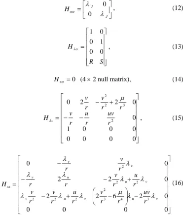
⎥ ⎦ ⎤ ⎢ ⎣ ⎡ = J J H λ λ αα 0 0 , (12) ⎥ ⎥ ⎥ ⎥ ⎥ ⎦ ⎤ ⎢ ⎢ ⎢ ⎢ ⎢ ⎣ ⎡ = S R H 0 0 1 0 0 1
λα , (13)
0
= α x
H (4 × 2 null matrix), (14)
⎥ ⎥ ⎥ ⎥ ⎥ ⎥ ⎦ ⎤ ⎢ ⎢ ⎢ ⎢ ⎢ ⎢ ⎣ ⎡ − − + − = 0 0 0 0 0 0 0 1 0 0 2 2 0 2 3 2 2 r uv r u r
v r r
v r v
Hx
µ
λ , (15)
⎥ ⎥ ⎥ ⎥ ⎥ ⎥ ⎥ ⎥ ⎦ ⎤ ⎢ ⎢ ⎢ ⎢ ⎢ ⎢ ⎢ ⎢ ⎣ ⎡ − ⎟⎟⎠ ⎞ ⎜⎜⎝ ⎛ − + − + − − − = 0 0 0 0 0 2 6 2 2 0 2 2 0 0 3 4 3 2 2 2 2 2 2 2 v u v u v v u u v v v xx r uv r r v r u r v r v r u r v r r r v r H λ λ µ λ λ λ λ λ λ λ λ λ (16)
Here, α denotes the control vector αT = [R S], x denotes the state vector xT = [u v r J ] and λ denotes the adjoint vector λT = [λu λv λr λJ].
From Eqs (5) and (6), one finds the functions Ψ and Φ :
⎥ ⎥ ⎥ ⎥ ⎥ ⎦ ⎤ ⎢ ⎢ ⎢ ⎢ ⎢ ⎣ ⎡ − − = f f f f f r t r r t v t u ) ( 1 ) ( ) (
Ψ , (17)
(
f f)
f f f
f r t r
r t v t u t
J + −
⎟⎟ ⎟ ⎠ ⎞ ⎜⎜ ⎜ ⎝ ⎛ − + +
= ( ) µ1 ( ) µ2 ( ) 1 µ3 ( )
Φ , (18)
where µi, i = 1, 2, 3, are Lagrangian multipliers associated to the final constraints defined by Eqs. (5) (or Eq(17) in a vector form); their partial derivatives are then given by
⎥ ⎥ ⎥ ⎦ ⎤ ⎢ ⎢ ⎢ ⎣ ⎡ = 0 1 0 0 0 0 1 0 0 0 0 1 x
Ψ , (19)
0
= xx
Φ . (4 × 4 null matrix). (20)
In the next section, the numerical results obtained through the proposed algorithm are presented.
Computational Results
The results of the numerical analysis obtained through the proposed algorithm for optimal low-thrust power limited trajectories considering simple transfers between coplanar circular orbits are presented for various radius ratios ρ = rf /r0 and for various transfer durations tf –t0. The set of several parameters used in the algorithm and first approximation of the control law have been chosen such that the admissible maximum number of iterations has been limited to 100 in all cases, the terminal constraints have been obtained with an error of 5.0 × 10⁻⁶, at least, that is, ⎜⎜Ψ(x(tf))⎜⎜≤ 5.0 × 10⁻⁶, with Ψ defined by Eq. (17) and the performance index has been calculated with an error e =⏐Jn+1 − Jn⏐< 5.0 × 10⁻¹⁰, where n denotes the iteration. This set of parameters is presented in Tables 1 and 2 following the nomenclature introduced in the companion paper: the parameters for steepest-descent phase are ki − weights of the penalty function; β − reduction factor for the step size in control space; K0− initial step size in control space; L − critic value used to redefine the step size in control space, and, the parameters for the second variation phase are k − reduction factor for partial corrections of the terminal constraint; ε − reduction factor for variations in control variables and Lagrange multipliers; Wii elements of the diagonal matrix W2 (used to assure Legendre condition). In Table 1, the ordinary parameters used for all values of ρ and tf –t0 are presented. Three different values of initial step size in control space have been used: K0 = 1.5 × 10⁻³ for ρ = 0.95, 0.975, 1.025, 1.050, 1.100, 1.200, K0 = 7.5 × 10⁻³ for ρ = 0.727, 1.523, K0 = 1.5 × 10⁻² for ρ = 0.800, 0.900. In Table 2, two different first approximations of the radial and circumferential components, R and
S, of the thrust acceleration are presented. Each computed maneuver
involves only one of these approximations. The second control law is used only for Earth-Venus transfers. It should be noted that the results do not represent the best performance of the proposed algorithm but they are acceptable, for the purposes of this analysis.
Table 1. Set of ordinary parameters.
k1,2,3 L k ε β Wu,2
200 5 000 0.175 0.25 0.75 −20 000
Table 2. First approximation of the thrust acceleration.
Thrust acceleration Control law 1 Control law 2
Radial - R Circumferential - S
0.0 1.0 × 10⁻⁵
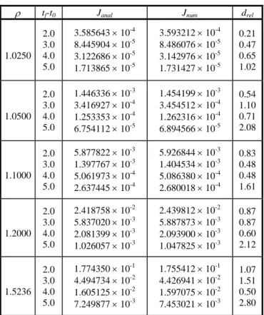
In Tables 3 and 4 the values of the consumption variable J computed through the proposed algorithm and the ones provided by a linear theory (Marec, 1979; Da Silva Fernandes 1989) are presented. The relative percent difference between the numerical and analytical results,
(
−)
/ ×100%= num anal anal
rel J J J
d ,
is, at least, about 3 % for ρ > 1 and 15 % for ρ < 1. A brief description of the linear theory is presented in the Appendix. The analytical expressions for the consumption variable and thrust acceleration provided by this linear theory involve the semi-major axis of a reference orbit O , which is taken as the middle value of the radii of the terminal orbits (Gobetz, 1965). From these results, one sees that the linear theory provides a good approximation for the solution of optimal transfer problem between close circular coplanar orbits: for the smaller amplitude transfers (⏐ρ −1⏐≤ 0.050), drel< 2.5 %, and, for the shorter duration transfers (tf − t0= 2), drel< 1.0 %.
Table 3. Consumption variable J (ρ > 1).
ρ tf-t0 Janal Jnum drel
1.0250 2.0 3.0 4.0 5.0
3.585643 × 10⁻⁴ 8.445904 × 10⁻⁵ 3.122686 × 10⁻⁵ 1.713865 × 10⁻⁵
3.593212 × 10⁻⁴ 8.486076 × 10⁻⁵ 3.142976 × 10⁻⁵ 1.731427 × 10⁻⁵
0.21 0.47 0.65 1.02
1.0500 2.0 3.0 4.0 5.0
1.446336 × 10⁻³ 3.416927 × 10⁻⁴ 1.253353 × 10⁻⁴ 6.754112 × 10⁻⁵
1.454199 × 10⁻³ 3.454512 × 10⁻⁴ 1.262316 × 10⁻⁴ 6.894566 × 10⁻⁵
0.54 1.10 0.71 2.08
1.1000 2.0 3.0 4.0 5.0
5.877822 × 10⁻³ 1.397767 × 10⁻³ 5.061973 × 10⁻⁴ 2.637445 × 10⁻⁴
5.926844 × 10⁻³ 1.404534 × 10⁻³ 5.086380 × 10⁻⁴ 2.680018 × 10⁻⁴
0.83 0.48 0.48 1.61
1.2000 2.0 3.0 4.0 5.0
2.418758 × 10⁻² 5.837020 × 10⁻³ 2.081399 × 10⁻³ 1.026057 × 10⁻³
2.439812 × 10⁻² 5.887873 × 10⁻³ 2.093900 × 10⁻³ 1.047825 × 10⁻³
0.87 0.87 0.60 2.12
1.5236 2.0 3.0 4.0 5.0
1.774350 × 10⁻¹ 4.494734 × 10⁻² 1.605125 × 10⁻² 7.249877 × 10⁻³
1.755412 × 10⁻¹ 4.426941 × 10⁻² 1.597075 × 10⁻² 7.453021 × 10⁻³
1.07 1.51 0.50 2.80
Table 4. Consumption variable J (ρ < 1).
ρ tf-t0 Janal Jnum drel
0.7270 2.0 3.0 4.0 5.0
3.765451 × 10⁻² 8.926982 × 10⁻³ 4.048203 × 10⁻³ 2.894188 × 10⁻³
3.777781 × 10⁻² 9.709937 × 10⁻³ 4.461201 × 10⁻³ 3.325080 × 10⁻³
0.33 8.77 10.20 14.88
0.8000 2.0 3.0 4.0 5.0
2.095182 × 10⁻² 4.904019 × 10⁻³ 2.070390 × 10⁻³ 1.383857 × 10⁻³
2.092074 × 10⁻² 5.053224 × 10⁻³ 2.196835 × 10⁻³ 1.505942 × 10⁻³
0.15 3.04 6.12 8.82
0.9000 2.0 3.0 4.0 5.0
5.474046 × 10⁻³ 1.277144 × 10⁻³ 5.006396 × 10⁻⁴ 3.049656 × 10⁻⁴
5.477794 × 10⁻³ 1.313377 × 10⁻³ 5.196754 × 10⁻⁴ 3.203318 × 10⁻⁴
0.07 2.84 3.80 5.04
0.9500 2.0 3.0 4.0 5.0
1.395891 × 10⁻³ 3.264941 × 10⁻⁴ 1.245127 × 10⁻⁴ 7.258595 × 10⁻⁵
1.396823 × 10⁻³ 3.302046 × 10⁻⁴ 1.265439 × 10⁻⁴ 7.378935 × 10⁻⁵
0.07 1.14 1.63 1.66
0.9750 2.0 3.0 4.0 5.0
3.522595 × 10⁻⁴ 8.255547 × 10⁻⁵ 3.112006 × 10⁻⁵ 1.776590 × 10⁻⁵
3.527534 × 10⁻⁴ 8.258122 × 10⁻⁵ 3.120254 × 10⁻⁵ 1.784648 × 10⁻⁵
0.14 0.03 0.26 0.45
t=2
t=3
t=4
t=5
Figure 2. Comparison between analytical and numerical results for consumption variable J (ρ > 1).
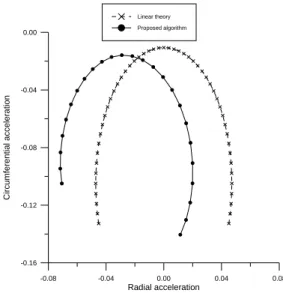
In order to follow the evolution of the optimal thrust acceleration vector during the transfer, it is also convenient to plot the locus of its tip in the moving frame of reference. Figures 12 – 15 illustrate the locii for Earth-Mars and Earth-Venus transfers for
tf − t0= 3 and tf − t0= 4. It should be noted that the agreement between the numerical and analytical results is better for Earth-Mars transfers.
t=2
t=3
t=4
t=5
Figure 3. Comparison between analytical and numerical results for consumption variable J (ρ < 1).
0.00 1.00 2.00 3.00
Normalized time
-0.40 -0.20 0.00 0.20 0.40
R
adi
al ac
cel
e
ra
tion
Linear theory Proposed algorithm
Figure 4. Radial acceleration history for ρ =1.523 and tf t0 = 3.
0.00 1.00 2.00 3.00
Normalized time
-0.10 0.00 0.10 0.20 0.30
C
ir
c
umfe
re
n
tial ac
cel
e
ra
ti
on
Linear theory Proposed algorithm
Figure 5. Circumferential acceleration history for ρ =1.523 and tf t0 = 3.
0.00 1.00 2.00 3.00
Normalized time
-0.10 -0.05 0.00 0.05 0.10
Radial
acce
lerati
o
n
Linear theory Proposed algorithm
0.00 1.00 2.00 3.00
Normalized time
-0.16 -0.12 -0.08 -0.04 0.00
Cir
c
umfer
e
n
tial accele
ra
tion
Linear theory Proposed algorithm
Figure 7. Circumferential acceleration history for ρ = 0.727 and tf t0 = 3.
0.00 1.00 2.00 3.00 4.00
Normalized time
-0.15 -0.10 -0.05 0.00 0.05 0.10
Ra
di
al acce
le
rat
io
n
Linear theory Proposed algorithm
Figure 8. Radial acceleration history for ρ =1.523 and tf t0 = 4.
0.00 1.00 2.00 3.00 4.00
Normalized time
-0.04 0.00 0.04 0.08 0.12 0.16
C
irc
umf
e
rent
ia
l acc
e
ler
a
tio
n Linear theory
Proposed algorithm
Figure 9. Circumferential acceleration history forρ =1.523 and tf t0 = 4.
0.00 1.00 2.00 3.00 4.00
Normalized time
-0.10 -0.05 0.00 0.05 0.10
R
adial accelerat
io
n
Linear theory Proposed algorithm
Figure 10. Radial acceleration history for ρ = 0.727 and tf t0 = 4.
0.00 1.00 2.00 3.00 4.00
Normalized time
-0.07 -0.06 -0.05 -0.04 -0.03 -0.02
Ci
rc
u
m
fe
re
nti
a
l a
c
c
e
le
ra
tio
n
Linear theory Proposed algorithm
Figure 11. Circumferential acceleration history for ρ = 0.727 and
tf t0 = 4.
-0.40 -0.20 0.00 0.20 0.40
Radial acceleration
-0.10 0.00 0.10 0.20 0.30
C
ir
c
umf
er
en
tia
l ac
cel
er
a
ti
on
Linear theory Proposed algorithm
-0.08 -0.04 0.00 0.04 0.08
Radial acceleration
-0.16 -0.12 -0.08 -0.04 0.00
Cir
c
umfe
ren
tial a
ccelera
tion
Linear theory Proposed algorithm
Figure 13. Thrust acceleration for ρ = 0.727 and tf t0 = 3.
-0.15 -0.10 -0.05 0.00 0.05 0.10
Radial acceleration
-0.04 0.00 0.04 0.08 0.12 0.16
C
ircum
ferential a
c
cele
ration
Linear theory Proposed algorithm
Figure 14. Thrust acceleration for ρ =1.523 and tf t0 = 4.
-0.02 -0.01 0.00 0.01 0.02
Radial acceleration
-0.07 -0.06 -0.05 -0.04 -0.03 -0.02
C
ir
c
um
fe
re
n
tia
l a
c
ce
le
ra
ti
on
Linear theory Proposed algorithm
Figure 15. Thrust acceleration for ρ = 0.727 and tf t0 = 4.
Conclusions
In this paper a gradient-based algorithm, presented in a companion paper, is applied to the analysis of optimal low-thrust limited-power transfers between close circular coplanar orbits in a Newtonian central gravity field. The numerical results provided by the algorithm have been compared to the analytical ones obtained by using a linear theory. The agreement between these results shows that the linear theory provides a good approximation for the solution of the transfer problem and can be used in preliminary mission analysis. The numerical and analytical results obtained in the paper also show that the fuel consumption can be greatly reduced if the duration of the transfer is increased: the fuel consumption for transfers with duration tf − t0= 2 is approximately ten times the fuel consumption for a transfer with duration tf − t0= 4. On the other hand, the performance of the proposed algorithm – accuracy in satisfying the terminal constraints, number of iterations to converge – shows that it is a good tool in determining optimal low-thrust limited-power trajectories between close circular orbits in a Newtonian central gravity field. The application of the algorithm to large amplitude transfers should be investigated. For further studies, the algorithm should be applied to numerical analysis of transfers between circular non-coplanar orbits and transfers between elliptical coplanar or non-coplanar orbits, for small and large amplitude transfers.
Acknowledgements
This research has been partially supported by CNPq under contract 300450/2003-6.
References
Coverstone-Carroll, V. and Williams, S.N., 1994, “Optimal Low Thrust Trajectories Using Differential Inclusion Concepts”, The Journal of the Astronautical Sciences, Vol 42, No 4, pp.379-393.
Coverstone-Carroll, V., Hartmann, J.W. and Mason, W.J., 2000, “Optimal Multi-Objective Low-Thrust Spacecrafts Trajectories”, Comput. Methods Appl. Mech. Engrg., No 186, pp. 387-402.
Da Silva Fernandes, S., 1989, “Optimal Low-Thrust Transfer between Neighboring Quasi-Circular Orbits around an Oblate Planet”, Acta Astronautica, Vol 19, pp. 933-939.
Da Silva Fernandes, S., and Golfetto, W. A., 2003, “Direct Methods in Numerical Computation of Optimal Trajectories”, Journal of Brazilian Society of Mechanical Sciences” (submitted).
Edelbaum, T.N., 1964, “Optimum Low-Thrust Rendez-vous and Station Keeping”, AIAA Journal, Vol 2, No 7, pp. 1196-1201.
Edelbaum, T.N., 1965, “Optimum Power-Limited Orbit Transfer in Strong Gravity Fields”, AIAA Journal, Vol 3, No 5, pp. 921-925.
Gobetz, F.W., 1965, “A Linear Theory of Optimum Low-Thrust Rendezvous Trajectories”, The Journal of the Astronautical Sciences, Vol 12, No 3, pp.69-76.
Geffroy, S. and Epenoy, R., 1997, “Optimal Low-Thrust Transfers with Constraints – Generalization of Averaging Techniques”, Acta Astronautica, Vol 41, pp. 133-149.
Haissig, C.M., Mease, K.D. and Vinh, N.X., 1992, “ Minimum-Fuel, Power-Limited Transfers Between Coplanar Elliptical Orbits”, Acta Astronautica, Vol 29, No 1, pp. 1-15.
Hestenes, M. R., 1969, “Multiplier and Gradient Methods”, Journal of Optimisation Theory and Applications, Vol.4, No. 5, pp.303-320.
Kechichian, J., 1996, “Optimal Low-Thrust Rendezvous Using Equinoctial Orbit Elements”, Acta Astronautica, Vol 38, No 1, pp. 1-14.
Kechichian, J., 1997, “Reformulation of Edelbaum’s Low-Thrust Transfer Problem Using Optimal Control Theory”, Journal of Guidance, Control and Dynamics, Vol 20, No 51, pp. 988-994.
Kechichian, J., 1998, “Orbit Raising with Low-Thrust Tangential Acceleration in Presence of Earth Shadow”, Journal of Spacecraft and Rockets, Vol 35, No 4, pp. 516-525.
Astrodynamics Specialist Conference, AAS Paper 97-717, Sun Valley, Idaho, August 4-7.
Marec, J. P., 1967, “Transferts Optimaux Entre Orbites Elliptiques Proches”, ONERA Publication n° 121, 254p.
Marec, J.P. and Vinh, N.X., 1977, “Optimal Low-Thrust, Limited Power Transfers between Arbitrary Elliptical Orbits”, Acta Astronautica, Vol 4, pp. 511-540.
Marec, J. P., 1979, “Optimal Space Trajectories”, Elsevier, New York, 329p.
O’Doherty, R.J. and Pierson, B.L., 1974, “A Numerical Study of Augmented Penalty Function Algorithms for Terminally Constrained Optimal Control Problems”, Journal of Optimisation Theory and Applications, Vol 14, No 4, pp.393-403.
Racca, G.D., 2001, “Capability of Solar Electric Propulsion for Planetary Missions”, Planetary Space Science, Vol 49, pp. 1437-144.
Racca, G.D., 2003, “New Challenges to Trajectory Design by the Use of Electric Propulsion and Other New Means of Wandering in the Solar System”, Celestial Mechanics and Dynamical Astronomy, Vol 85, pp. 1-24.
Sukhanov, A.A. and Prado, A.F.B. de A., 2001, “Constant Tangential Low-Thrust Trajectories near an Oblate Planet”, Journal of Guidance, Control and Dynamics, Vol 24, No 4, pp. 723-731.
Vasile, M., Bernelli Zazzera, F., Jehn, R. and G., Janin, G., 2000, “Optimal Interplanetary Trajectories Using a Combination of Low-Thrust and Gravity Assist Manoeuvres”, IAF-00-A.5.07, 51th IAF Congress, Rio de Janeiro, Brazil.
Appendix
A first order analytical solution for the problem of optimal simple transfer (no rendezvous) between close quasi-circular coplanar orbits in a Newtonian central gravity fields is given by (Edelbaum, 1964; Marec, 1967, 1979; Da Silva Fernandes, 1989):
0
λ
∆x=A , (A.1)
where ∆x = [∆α ∆h ∆k ]T denotes the imposed changes on non-singular orbital elements (state variables): α=a /a, h = ecosω, k =
esinω, where a is the semi-major axis, e is the eccentricity and ω is the argument of the pericenter; λ0 is the 3 × 1 vector of initial values of the adjoint variables, and, A is a 3 × 3 symmetric matrix. The overbar denotes the reference orbit O about which the linearization is done. In this first order solution, the adjoint variables associated to the non-singular elements are constant. The matrix A is given by:
⎥ ⎥ ⎥ ⎦ ⎤ ⎢ ⎢ ⎢ ⎣ ⎡ = kk kh k hk hh h k h a a a a a a a a a A α α α α αα , (A.2) where: , 4 3 5 A ∆ µ αα a
a = (A.3)
(
0)
3 5
sin sin
4 A − A
=
= h f
h a a a µ α
α , (A.4)
(
0)
3 5
cos cos
4 A − A
− =
= k f
k a a a µ α
α , (A.5)
(
)
⎥⎦⎤⎢⎣
⎡ + −
= 3 0
5 2 sin 2 sin 4 3 2 5 A A A f hh a a ∆
µ , (A.6)
(
0)
3 5 2 cos 2 cos 4 3 A A − − =
= kh f
hk
a a
a
µ , (A.7)
(
)
⎥⎦⎤⎢⎣
⎡ − −
= 3 0
5 2 sin 2 sin 4 3 2 5 A A A f kk a a ∆
µ , (A.8)
where Af =A0+n
(
tf −t0)
=A0+∆A, t0 is the initial time, tf is the final time, 3a
n= µ is the mean motion (reference orbit O ).
The optimal thrust acceleration Γ∗ and the variation of the consumption variable J∆ during the maneuver is expressed by:
(
) (
)
{
h k r h k es}
a
n sinA cosA 2 cosA sinA
1
λ λ
λ λ
λ − + α+ +
=
∗ e
Γ , (A.9)
{
}
2 2 2 2 2 2 2 1 k kk k h hk h hh k k h h a a a a a a J λ λ λ λ λ λ λ λ λ∆ αα α α α α α
+ + + + + + =
, (A.10)
where aaa, aαh,…, akk are given by Eqns (A.3) - (A.8), and, λα , λh, and λk are obtained from the solution of the linear algebraic system defined by Eq. (A.1); er and es are unit vectors extending along
radial and circumferential directions in a moving reference frame, respectively.
For transfers between circular orbits, only ∆α is imposed. If it is assumed that the initial and final positions of the vehicle in orbit are symmetric with respect to x-axis of the inertial reference system, that is, Af =−A0=∆A 2, the solution of the system (A.1) is given
by:
(
)
( )
⎭⎬ ⎫ ⎩ ⎨ ⎧ − + + = 2 sin 64 sin 6 10 sin 3 5 2 1 2 2 5 3 A A A A A A ∆ ∆ ∆∆ ∆α ∆ ∆
µ λα
a , (A.11)
( )
⎭⎬ ⎫ ⎩ ⎨ ⎧ − + − = 2 sin 64 sin 6 10 2 sin 8 2 2 5 3 A A A A A ∆ ∆ ∆∆ ∆α ∆
µ λ
a
h , (A.12)
0
= k
λ , (A.13)
Note that the particular choice of the x-axis is possible because the primary body has z-axis symmetry.