Rev. bras. meteorol. vol.29 número4

(1)

Revista Brasileira de Meteorologia, v.29, n.4, 469 - 482, 2014 http://dx.doi.org/10.1590/0102-778620120568

ESTIMATION OF SOIL HEAT FLUX IN A NEOTROPICAL WETLAND REGION USING REMOTE

SENSING TECHNIQUES

VICTOR HUGO DE MORAIS DANELICHEN

1

, MARCELO SACARDI BIUDES

1

,

MAÍSA CALDAS SOUZA

1

, NADJA GOMES MACHADO

1,2

,

BERNARDO BARBOSA DA SILVA

3

, JOSÉ DE SOUZA NOGUEIRA

1

Universidade Federal de Mato Grosso (UFMT), Instituto de Física, Cuiabá, MT, Brazil

2

Instituto Federal de Mato Grosso, Laboratório da Biologia da Conservação, Campus Bela Vista, Cuiabá,

MT, Brazil

3

_{Universidade Federal de Pernambuco (UFPE), Departamento de Geograia e Recursos Hídricos, Recife,}

PE, Brazil

danelichen@isica.ufmt.br

,

marcelo@isica.ufmt.br

,

maisacaldas@isica.ufmt.br

,

nadja.machado@blv.ifmt.edu.br

,

bbdasilva.ufpe@gmail.com

,

nogueira@ufmt.br

Received November 2012 - Accepted February 2014

ABSTRACT

The direct estimation of the soil heat lux (G) by remote sensing data is not possible. For this, several models have been proposed empirically from the relation of G measures and biophysical parameters of various types of coverage or not vegetated in different places on earth. Thus, the objective of this study was to evaluate the relation between G/Rn ratio and biophysical variables obtained by satellite sensors and evaluate the parameterization of different models to estimate G spatially in three sites with different soil cover types. The net radiation (Rn) and G were measured directly in two pastures at Miranda Farm and Experimental Farm and and Monodominant Forest of Cambará. Rn, G, and G/Rn ratio and MODIS products, such as albedo (α), surface temperature (LST), vegetation index (NDVI) and leaf area index (LAI) varied seasonally at all sites and inter-sites. The sites were different from each other by presenting different relation between measures of Rn, G and G/Rn ratio and biophysical parameters. Among the original models, the model proposed by Bastiaanssen (1995) showed the best performance with r = 0.76, d = 0.95, MAE= 5.70 W m-2 and RMSE = 33.68 W m-2. As the reparameterized models, correlation coeficients had no signiicant change, but the coeficient Willmott (d) increased and the MAE and RMSE had a small decrease.

Keywords: Mato Grosso, pasture, monodominant forest, orbital sensors.

RESUMO: PARAMETRIZAÇÃO DE MODELOS PARA ESTIMAR O FLUXO DE CALOR NO SOLO EM TRÊS REGIÕES DO PANTANAL DO MATO GROSSO USANDO SENSORIAMENTO REMOTO

(2)

470 Danelichen et al. Volume 29(4)

parâmetros biofísicos. Dentre os modelos originais, o modelo proposto por Bastiaanssen (1995) apresentou o melhor desempenho com r = 0,76, d = 0,95, MAE = 5,70 W m-2_{e RMSE = 33,68} W m-2. Quanto aos modelos reparametrizados, os coeicientes de correlação se mantiveram, mas o coeiciente de Willmott (d) aumentou e o MAE e RMSE tiveram uma pequena diminuição. Palavras-chave: Mato Grosso, pastagens, loresta monodominante, sensores orbitais.

1. INTRODUCTION

The Mato Grosso State has a rich ecological diversity in three distinct biomes (Amazon, Pantanal and Cerrado), which have special importance on global climatic changes issues (Arieira et al., 2011). Recent trends of economic development have contributed to convert natural areas in pasture and cropland (Wantzen et al., 2008; Milne et al., 2010). This landscape conversion changes the energy exchange of the soil-plant-atmosphere system (Coutinho, 2010).

The assessment of energy exchange can be carried by micrometeorological techniques, which allows the characterization of local microclimate, as well the identiication of the ecosystem function changes caused by anthropogenic activities (Biudes et al., 2009). However, these technics provide a punctual measure of the energy exchange and its use to spatial characterization is expensive and laboriously. Therefore, remote sensing techniques are highlighted because they allow monitoring of energy exchange on a regional scale using a few ground data (Allen et al., 2011).

Actually, different methodologies to estimate the energy exchange by remote sensing techniques are used (Bastiaanssen et al., 2005; Mu et al., 2007; Allen et al., 2007; Kustas and Anderson, 2009). The Surface Energy Balance Algorithm for Land (SEBAL; see Bastiaanssen 2000; Bastiaanssen et al., 2005) is a model used to several issues (Bastiaanssen, 1995; Bastiaanssen et al., 2005; Allen et al., 2011). However, the effectiveness of this model over different geographical areas depends of the correct soil heat lux (G) estimation (Kustas and Norman, 1999).

The G is a function of the soil-plant system coniguration, and it varies according to the soil type and water content (Bezerra et al., 2008), vegetation type (Allen et al., 2005; Santos et al., 2010) and local microclimate (Allen et al., 2007). Generally, the G represents 5% of net radiation (Rn) in forest and between 20 and 40% in partially covered surface (Kustas et al., 2000). Due to the amplitude of variation of G and G/Rn ratio, this issue requires more attention (Payero et al., 2005).

The G cannot be directly mapped by satellite observations (Allen et al., 2011), but the fraction G/Rn is reasonably predictable near to noon by the empirical relation with soil and vegetation characteristic estimated by satellite image data (Choudhury et al., 1987; Bastiaanssen, 1995; Tasumi, 2003, Allen et al., 2011), such as the leaf area index (LAI), normalized

difference vegetation index (NDVI), albedo (α) and land-surface temperature (LST). Thus, several models have been proposed to estimate G based on the G/Rn ration as a function soil and vegetation characteristics (Choudhury et al., 1987; Jackson et al., 1987; Kustas and Daughtry, 1990; Kustas et al., 1993; Bastiaassen, 1995; Burba et al., 1999; Ma et al., 2001; Payero et al., 2001; Tasumi, 2003; Ruhoff, 2011). However, these methods were formulated for different types of surfaces (soil and vegetation) in different locations.

Therefore, the objective of this study was evaluate the relation between G/Rn ratio and satellite image data and evaluate the parameterization of different models to estimate G spatially in three different sites in Mato Grosso state.

2. MATERIALS AND METHODS

2.1 Sites description

The study was conducted in three different sites in Mato Grosso state (Figure 1) with similar climate characteristics. The annual average of temperature is 24.9-25.4°C, precipitation is 1300-1400 mm, and there is a dry season between April and September, and a wet season from October to March (SEPLAN, 2001). The irst area is located on Miranda Farm (MF) in Cuiaba-MT, and coordinates 15° 43’ 53, 65’’ S and 56º 04’ 18, 88’’ W and the altitude of 157 m. This area is characterized as a pasture, with dominance of herbaceous vegetation that emerged after the deforestation, and it contains Cerrado stricto sensu fragments. The soil of Miranda Farm was classiied as

PLINTOSSOLO PÉTRICO Concrecionário lítico.

The second area was located at the Experimental Farm (EF) of the Federal University of Mato Grosso, with coordinates 15° 47’ 11 “S and 56º 04’ 47” W and altitude of 140 m, in Santo Antônio do Leverger-MT. This area is characterized as a Brachiaria humidicola pasture. The soil was classiied as

PLANOSSOLO HÁPLICO Eutróico gleissólico.

(3)

Dezembro 2014 Revista Brasileira de Meteorologia 471

All sites had the same equipment description. The net radiation was measured by a net radiometer (NR-LITE, Kipp & Zonen Delft, Inc., Holland) installed at 5 m in MF, 2.5 m in EF and 33 m in CAM above the vegetation canopy, and the soil heat lux were obtained by soil heat lux plates (model HFT-3.1, Rebs, Inc., Seattle, Washington) installed at 2 cm deep surface. The produced data from the transducers in all sites were processed and stored every 15 minutes by a datalogger (CR 10X, Campbell Scientiic, Inc., Logan, Utah).

2.3 Estimation of soil heat lux by different methods using remote sensing data

We downloaded the leaf area index - LAI (MOD15A2), land-surface temperature - LST (MOD11A2), albedo - α (MCD43A3) and normalized difference vegetation index - NDVI (MOD13Q1), based on the geo-location information (latitude and longitude) of each area. The time series used were between 2009 and 2011, only 2007, and 2007 and 2008 to FM, FE and CAM, respectively. The data are published by the EROS Data Center Active Archive Center (EDC Daac). As noise in vegetation index should be low and the spatial resolution of each MODIS product, we used a pixel group as a guarantee of high quality metric (QA) to obtain the average MODIS products, representing of 1 km2 around each tower. Only pixels with highest quality assurance metrics were used to parameterize the models to estimate G.

There were some data gaps even using pixel groups. The presence of cloud and aerosols and the variation caused

by bidirectional relectance and sensor geometry can limit the relectance eficacy to assess spatial-temporal dynamics in biophysical processes (Hird and McDermid, 2009). To improve the signal-noise ratio we use a signal extraction technique (Hermance et al., 2007). Thus, we applied Singular Spectrum Analysis, using the CatMV software (Golyandina and Osipova, 2007), which is particularly effective for the iltered reconstruction of short, irregularly spaced, and noisy time series (Ghil et al., 2002; Golyandina and Osipova, 2006) to improve the signal-noise ratio of the MODIS land surface relectance.

The soil heat lux (G) was estimated by different models, such as Choudhury et al. (1987) (Equation 1); Jackson et al. (1987) (Equation 2); Kustas and Daughtry, (1990) (Equation 3); Kustas et al. (1993) to LAI < 4 (Equation 4); Kustas et al. (1993) to LAI > 4 (Equation 5); Bastiaanssen (1995) (Equation 6); Burba et al. (1999) (Equation 7); Payero et al. (2001) (Equation 8); Ma et al. (2001) (Equation 9); Tasumi (2003) to vegetated soil (Equation 10); Tasumi (2003) to bare soil (Equation 11); and Ruhoff (2011) (Equation 12).

Figure 1 - Location of Mato Grosso, Brazil experimental sites in a Monodominant Forest of Cambará (CAM), Miranda Farm (MF) and Experimental

Farm (EF).

 =  × 0.4 ×  −0.5 × 

 =  × 0.583 × −2.13 × 

 =  × 0.32 − 0.21 × 

 =  × 0.34 × −0.46 × 

 =  × 0.07

 =  ×  − 273.16 × 0.0038 + 0.0074 ×  × 1 − 0.98 × _

 = 0.41 ×  − 51

 =  × −13.46 + 0.507 × 4 × 0.123 ×  − 273.16 + 0.0863

 = 0.35 ×  − 47.79

 =  × 0.05 + 0.18 × −0.521 × 

 = 1.8 ×  − 273.16  + 0.084

 = 0.007 ×  + 0.95 ×  − 273.16 − 23.21

(1) =  × 0.4 ×  −0.5 × 

 =  × 0.583 × −2.13 × 

 =  × 0.32 − 0.21 × 

 =  × 0.34 × −0.46 × 

 =  × 0.07

 =  ×  − 273.16 × 0.0038 + 0.0074 ×  × 1 − 0.98 × _

 = 0.41 ×  − 51

 =  × −13.46 + 0.507 × 4 × 0.123 ×  − 273.16 + 0.0863

 = 0.35 ×  − 47.79

 =  × 0.05 + 0.18 × −0.521 × 

 = 1.8 ×  − 273.16  + 0.084

 = 0.007 ×  + 0.95 ×  − 273.16 − 23.21

(2)

 =  × 0.4 ×  −0.5 × 

 =  × 0.583 × −2.13 × 

 =  × 0.32 − 0.21 × 

 =  × 0.34 × −0.46 × 

 =  × 0.07

 =  ×  − 273.16 × 0.0038 + 0.0074 ×  × 1 − 0.98 × _

 = 0.41 ×  − 51

 =  × −13.46 + 0.507 × 4 × 0.123 ×  − 273.16 + 0.0863

 = 0.35 ×  − 47.79

 =  × 0.05 + 0.18 × −0.521 × 

 = 1.8 ×  − 273.16  + 0.084

 = 0.007 ×  + 0.95 ×  − 273.16 − 23.21

(3)

 =  × 0.4 ×  −0.5 × 

 =  × 0.583 × −2.13 × 

 =  × 0.32 − 0.21 × 

 =  × 0.34 × −0.46 × 

 =  × 0.07

 =  ×  − 273.16 × 0.0038 + 0.0074 ×  × 1 − 0.98 × _

 = 0.41 ×  − 51

 =  × −13.46 + 0.507 × 4 × 0.123 ×  − 273.16 + 0.0863

 = 0.35 ×  − 47.79

 =  × 0.05 + 0.18 × −0.521 × 

 = 1.8 ×  − 273.16  + 0.084

 = 0.007 ×  + 0.95 ×  − 273.16 − 23.21  =  × 0.4 ×  −0.5 × 

 =  × 0.583 × −2.13 × 

 =  × 0.32 − 0.21 × 

 =  × 0.34 × −0.46 × 

 =  × 0.07

 =  ×  − 273.16 × 0.0038 + 0.0074 ×  × 1 − 0.98 × _

 = 0.41 ×  − 51

 =  × −13.46 + 0.507 × 4 × 0.123 ×  − 273.16 + 0.0863

 = 0.35 ×  − 47.79

 =  × 0.05 + 0.18 × −0.521 × 

 = 1.8 ×  − 273.16  + 0.084

 = 0.007 ×  + 0.95 ×  − 273.16 − 23.21

(4)

All models relate the G/Rn ratio and biophysical parameters, which were used the MODIS products of LAI (MOD15A2), LST (MOD11A2), α (MCD43A3) and NDVI (MOD13Q1). The average of micrometeorological data (Rn, G and the ratio G/Rn) obtained between 9:30 min and 13:30 min were synchronized with the MODIS products for each site according to data availability.

2.5 Analysis of statistical data

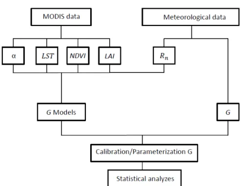
The general concept of the method is shown in Figure 2. The α, LST, NDVI and LAI obtained as MODIS products were combined with G/Rn obtained in each area. The parameterizations of the models were performed using a nonlinear regression by G/Rn ratio as the dependent variable and MODIS products as independent variables (Wilks, 2011).

The evaluation of parametrization was performed by Pearson correlation (r), Willmott index (d), root mean square error (RMSE) and mean absolute error (MAE) (Willmott et al., 1985; Willmott and Matsuura, 2005). The Kruskal-Wallis test (Wilks, 2011) was used to verify which variables were signiicant differences between the study sites (FM, FE and CAM). The Mann Whitney test (Wilks, 2011) was used to verify if the period of data collection (the rainy season from October to April, and dry season from May to September) caused signiicant variations (p-value <0.05) in Rn, G, G/Rn, α, LST, NDVI and LAI.

3. RESULTS AND DISCUSSION

3.1 Evaluation of products obtained from orbital

sensors

The α (Figure 3 and Table 1) were significantly affected by sites and seasons (p-value<0.05). The highest α

values in MF and EF are due to smaller, sparse and lighter vegetation which increases the relection power of surface affecting directly albedo estimative (Doughty et al., 2012), representing 19-27% of incoming short wave radiation (Breuer et al., 2003). On the other hands, forested surfaces have lower α (11-14%) and more uneven canopies compared to pastures, absorbing more sunlight and facilitating the mix of air (Breuer et al., 2003). Forested areas have higher surface roughness and moisture, and dark color than the pastures, which directly inluences the uptake of energy relected and absorbed by the earth’s surface (Berbet and Costa, 2003). Moreover, the CAM vegetation structure is 28-30 m trees height which provides a greater absorption of solar radiation that penetrates the canopy and is absorbed therein (Allen, 2007; Ruhoff, 2011, Santos et al., 2011). The conversion of forest to short vegetation is associated with signiicant increase in α and a consequent reduction in the net energy absorbed by the canopy (Culf et al., 1995), which decrease in rugosity, root system and foliar surface (Sheil and Murdiyarso 2009).

The α values were also higher during dry season in all sites (Table 1). The seasonality of α is a function of precipitation in all sites, which has a strong seasonal trend with 90% of total precipitation occurring during the wet season (Biudes et al., 2013). The higher α during the dry season is due to the dry surface areas with lighter coloration, whereas the surfaces (vegetation and soil) are dark during the wet season (Santos et al., 2011).

The LST was positively correlated with α in all sites (Table 2). The LST (Figure 3 and Table 1) were signiicantly affected by sites and seasons (p-value <0.05). CAM was cooler than MF and EF, and the LST was higher during wet season. The spatial variation in LST is the result of a complex combination of intrinsic factors (soil and vegetation types, bedrock, etc.) and extrinsic factors (topography, sunlight, proximity of targets, etc.), which result on the variation of the regional optical characteristics (Santos et al., 2011). The lower values of LST in CAM (Table 1) were due to the barrier imposed by the vegetation canopy, which reduces the solar irradiative transfer (Santos et al., 2011). Furthermore, the forest reduces sensible heat luxes which typically comes at a cost of evaporating more water. Thus, the degree of this cooling is regulated by constraints such as leaf area, rooting depth and soil water availability (Nosetto et al. 2012). From an aerodynamic perspective, a closer coupling of LST and air temperature occurs due to a strong mixing between air and forested surfaces. The reduction on LST in all sites during dry season is a function of the decreasing of incoming solar radiation and the occurrence of the “friagens” in the region (Biudes et al., 2012).

 =  × 0.4 ×  −0.5 × 

 =  × 0.583 × −2.13 × 

 =  × 0.32 − 0.21 × 

 =  × 0.34 × −0.46 × 

 =  × 0.07

 =  ×  − 273.16 × 0.0038 + 0.0074 ×  × 1 − 0.98 × _

 = 0.41 ×  − 51

 =  × −13.46 + 0.507 × 4 × 0.123 ×  − 273.16 + 0.0863

 = 0.35 ×  − 47.79

 =  × 0.05 + 0.18 × −0.521 × 

 = 1.8 ×  − 273.16  + 0.084

 = 0.007 ×  + 0.95 ×  − 273.16 − 23.21  =  × 0.4 ×  −0.5 × 

 =  × 0.583 × −2.13 × 

 =  × 0.32 − 0.21 × 

 =  × 0.34 × −0.46 × 

 =  × 0.07

 =  ×  − 273.16 × 0.0038 + 0.0074 ×  × 1 − 0.98 × _ ₍

 = 0.41 ×  − 51

 =  × −13.46 + 0.507 × 4 × 0.123 ×  − 273.16 + 0.0863

 = 0.35 ×  − 47.79

 =  × 0.05 + 0.18 × −0.521 × 

 = 1.8 ×  − 273.16  + 0.084

 = 0.007 ×  + 0.95 ×  − 273.16 − 23.21

 =  × 0.4 ×  −0.5 × 

 =  × 0.583 × −2.13 × 

 =  × 0.32 − 0.21 × 

 =  × 0.34 × −0.46 × 

 =  × 0.07

 =  ×  − 273.16 × 0.0038 + 0.0074 ×  × 1 − 0.98 × _

 = 0.41 ×  − 51

 =  × −13.46 + 0.507 × 4 × 0.123 ×  − 273.16 + 0.0863

 = 0.35 ×  − 47.79

 =  × 0.05 + 0.18 × −0.521 × 

 = 1.8 ×  − 273.16  + 0.084

 = 0.007 ×  + 0.95 ×  − 273.16 − 23.21

 =  × 0.4 ×  −0.5 × 

 =  × 0.583 × −2.13 × 

 =  × 0.32 − 0.21 × 

 =  × 0.34 × −0.46 × 

 =  × 0.07

 =  ×  − 273.16 × 0.0038 + 0.0074 ×  × 1 − 0.98 × _

 = 0.41 ×  − 51

 =  × −13.46 + 0.507 × 4 × 0.123 ×  − 273.16 + 0.0863

 = 0.35 ×  − 47.79

 =  × 0.05 + 0.18 × −0.521 × 

 = 1.8 ×  − 273.16  + 0.084

 = 0.007 ×  + 0.95 ×  − 273.16 − 23.21  =  × 0.4 ×  −0.5 × 

 =  × 0.583 × −2.13 × 

 =  × 0.32 − 0.21 × 

 =  × 0.34 × −0.46 × 

 =  × 0.07

 =  ×  − 273.16 × 0.0038 + 0.0074 ×  × 1 − 0.98 × _

 = 0.41 ×  − 51

 =  × −13.46 + 0.507 × 4 × 0.123 ×  − 273.16 + 0.0863

 = 0.35 ×  − 47.79

 =  × 0.05 + 0.18 × −0.521 × 

 = 1.8 ×  − 273.16  + 0.084

 = 0.007 ×  + 0.95 ×  − 273.16 − 23.21  =  × 0.4 ×  −0.5 × 

 =  × 0.583 × −2.13 × 

 =  × 0.32 − 0.21 × 

 =  × 0.34 × −0.46 × 

 =  × 0.07

 =  ×  − 273.16 × 0.0038 + 0.0074 ×  × 1 − 0.98 × _

 = 0.41 ×  − 51

 =  × −13.46 + 0.507 × 4 × 0.123 ×  − 273.16 + 0.0863

 = 0.35 ×  − 47.79

 =  × 0.05 + 0.18 × −0.521 × 

 = 1.8 ×  − 273.16  + 0.084

 = 0.007 ×  + 0.95 ×  − 273.16 − 23.21  =  × 0.4 ×  −0.5 × 

 =  × 0.583 × −2.13 × 

 =  × 0.32 − 0.21 × 

 =  × 0.34 × −0.46 × 

 =  × 0.07

 =  ×  − 273.16 × 0.0038 + 0.0074 ×  × 1 − 0.98 × _

 = 0.41 ×  − 51

 =  × −13.46 + 0.507 × 4 × 0.123 ×  − 273.16 + 0.0863

 = 0.35 ×  − 47.79

 =  × 0.05 + 0.18 × −0.521 × 

 = 1.8 ×  − 273.16  + 0.084

 = 0.007 ×  + 0.95 ×  − 273.16 − 23.21  =  × 0.4 ×  −0.5 × 

 =  × 0.583 × −2.13 × 

 =  × 0.32 − 0.21 × 

 =  × 0.34 × −0.46 × 

 =  × 0.07

 =  ×  − 273.16 × 0.0038 + 0.0074 ×  × 1 − 0.98 × _

 = 0.41 ×  − 51

 =  × −13.46 + 0.507 × 4 × 0.123 ×  − 273.16 + 0.0863

 = 0.35 ×  − 47.79

 =  × 0.05 + 0.18 × −0.521 × 

 = 1.8 ×  − 273.16  + 0.084

 = 0.007 ×  + 0.95 ×  − 273.16 − 23.21  =  × 0.4 ×  −0.5 × 

 =  × 0.583 × −2.13 × 

 =  × 0.32 − 0.21 × 

 =  × 0.34 × −0.46 × 

 =  × 0.07

 =  ×  − 273.16 × 0.0038 + 0.0074 ×  × 1 − 0.98 × _

 = 0.41 ×  − 51

 =  × −13.46 + 0.507 × 4 × 0.123 ×  − 273.16 + 0.0863

 = 0.35 ×  − 47.79

 =  × 0.05 + 0.18 × −0.521 × 

 = 1.8 ×  − 273.16  + 0.084

 = 0.007 ×  + 0.95 ×  − 273.16 − 23.21

(5)

The α and LST were delayed in time, for eight days in MF, sixteen days in EF and eight days in CAM (Figure 3). These delays were possibly by the different time interval of the surface absorption of incident irradiation and atmospheric interaction. This irradiation passes downward through the atmosphere before being captured by the orbital sensor and then return to it (Mu et al., 2011).

The NDVI and LAI were positively correlated in MF and EF and were not correlated in CAM (Table 2). These differences are probably related to their distant mathematical formulations and present different spectral characteristics (Heute, 2002). The largest NDVI and LAI amplitude occurs in MF and EF, while these indexes do not show any appreciable changes in CAM (Table 1).

Figure 2 - Diagram of the procedure for parameterizing the soil heat lux (G) combining MODIS products as albedo (α), land surface temperature (LST), leaf area index (LAI), normalized difference index (NDVI ) and net radiation (Rn).

Local Season Rn

(W m-2)

G

(W m-2)

G/Rn α

LST

(°C)

NDVI

LAI

(m2 m-2)

MF

Dry 430,5±39,2 102,0±16,0 0,243±0,050 0,215±0,017 33,1±2,2 0,489±0,065 1,2±0,2

Wet 532,6±68,4 94,3±35,6 0,180±0,060 0,214±0,019 32,0±1,6 0,623±0,037 1,8±0,2

EF

Dry 434,4±42,6 31,6±7,5 0,073±0,018 0,231±0,015 31,9±2,6 0,533±0,056 1,3±0,2

Wet 520,5±83,7 37,3±7,0 0,070±0,007 0,226±0,017 31,1±1,1 0,642±0,039 2,0±0,1

CAM

Dry 399,4±63,2 10,1±1,9 0,025±0,004 0,202±0,007 28,7±1,9 0,794±0,003 6,0±0,2

Wet 512,8±64,6 7,1±1,2 0,013±0,003 0,212±0,006 28,6±1,9 0,819±0,013 6,1±0,1

(6)

The NDVI and LAI were signiicantly affected by sites and seasons (p-value <0.05) (Figure 3 and Table 1). There was no difference of NDVI and LAI values between MF and EF, and they were lower than CAM (Table 1). The lower values of NDVI and LAI in MF and EF in the dry season indicate that the photosynthetic activate was impacted by the hydric stress due to less rainfall (Huete et al., 2006). The higher vegetation biomass relects more near-infrared radiation during the wet season, which inluences in NDVI increase (Mu et al., 2011). The relationship between NDVI and vegetation structural parameters, such as biomass and LAI, which is a biophysical variable directly, related to transpiration and forest productivity shows up better for areas of early succession in presenting lower values of biomass

(Breda et al., 2003). The smallest differences of NDVI and LAI on CAM were due to the better adaptation strategy of the vegetation. The overstory LAI and understory LAI of CAM have an inverse seasonal pattern with higher overstory LAI in wet season and higher understory LAI during the dry season, and the result is a lack of seasonal signiicance of total LAI (Biudes et al., 2013).

3.2 Evaluation of the soil heat lux and radiation balance

The average of net radiation (Rn) obtained between 9:30 min and 13:30 min of each day (Figure 4 and Table 1) was not signiicant affected by sites, but it was signiicantly

out/09 jan/10 abr/10 jul/10 out/10 jan/11 abr/11

Land S ur fac e T em pe rat ur e ( °C ) 24 26 28 30 32 34 36 38 LST A lbedo 0.18 0.19 0.20 0.21 0.22 0.23 0.24 0.25 Albedo a

out/09 jan/10 abr/10 jul/10 out/10 jan/11 abr/11

Leaf A rea Index LA I (m

2 m -2 ) 0 1 2 3 4 5 6 7 LAI N or m a liz ed D if fer enc e V eg et at ion I nde x N D V I 0.40 0.45 0.50 0.55 0.60 0.65 0.70 0.75 0.80 0.85 NDVI b

fev/07 abr/07 jun/07 ago/07 out/07 dez/07 24 26 28 30 32 34 36 38 0.18 0.19 0.20 0.21 0.22 0.23 0.24 0.25

fev/07 abr/07 jun/07 ago/07 out/07 dez/07 0.40 0.45 0.50 0.55 0.60 0.65 0.70 0.75 0.80 0.85 0 1 2 3 4 5 6 7 Month/Year

jun/07 ago/07 out/07 dez/07 fev/08 24 26 28 30 32 34 36 38 0.18 0.19 0.20 0.21 0.22 0.23 0.24 0.25

jun/07 ago/07 out/07 dez/07 fev/08 0 1 2 3 4 5 6 7 0.40 0.45 0.50 0.55 0.60 0.65 0.70 0.75 0.80 0.85 c d e f

(7)

Miranda Farm

G Rn G/Rn α LST NDVI LAI

G 1.00

Rn 0.32*

1.00

G/Rn 0.83* -0.24 1.00

α 0.75* 0.09 0.73* 1.00

LST 0.69*

-0.13 0.80*

0.84*

1.00

NDVI -0.43* 0.50* -0.74* -0.39* -0.67* 1.00

LAI -0.47* 0.41* -0.73* -0.44* -0.58* 0.91* 1.00

Experimental Farm

G Rn G/Rn α LST NDVI LAI

G 1.00

Rn 0.65* 1.00

G/Rn 0.72*

-0.05 1.00

α 0.24 -0.38* 0.64* 1.00

LST 0.52*

-0.07 0.76*

0.51*

1.00

NDVI 0.07 0.57*

-0.44*

-0.49*

-0.46*

1.00

LAI 0.35* 0.56* -0.08 -0.04 -0.06 0.78* 1.00

Monodominant Forest of Cambará

G Rn G/Rn α LST NDVI LAI

G 1.00

Rn -0.39* 1.00

G/Rn 0.82*

-0.72*

1.00

α -0.35 0.11 -0.50* 1.00

LST 0.10 -0.08 -0.09 0.69* 1.00

NDVI -0.80*

0.76*

-0.86*

0.18 -0.20 1.00

LAI -0.13 0.12 -0.39* 0.83* 0.76* 0.09 1.00

Table 2 - Spearman correlation matrix of soil heat lux (G), net radiation (Rn), G/Rn ratio, albedo (α), land-surface temperature (LST), normalized difference vegetation index (NDVI) and leaf area index (LAI) of the Miranda Farm (MF), Experimental Farm (EF) and Monodominant Forest of

Cambará (CAM). The symbol (*) indicates p-value < 0.05.

affected by seasons (p-value<0.05). The higher values of Rn occurs in the wet season due to astronomical factors, which reduce the solar radiation in June and increase to a maximum in December (Biudes et al., 2009). Furthermore, the forest degradation and deforestation can expose the soil and affect the long wave balance due to the release of particulate matter into the atmosphere during dry season (Betts et al., 2008), and decrease the incoming solar radiation due to changes in the chemical atmosphere composition with the emission of trace gases and aerosol particles (Artaxo et al., 2006). Another Rn variation cause variation is the spectral characteristics of the surface of study areas (Rodrigues et al., 2009). However, as there was no interaction between sites and seasons, we cannot point to surface spectral characteristics as a cause of Rn variation. The Rn was positively correlated with NDVI in all areas, and negatively correlated with α in EF (Table 2). The positive correlation of NDVI with Rn is the coincidence of the occurrence of intense sunlight and high water availability during wet season (Table 2).

The average of soil heat lux (G) obtained between 9:30 min and 13:30 min of each day (Figure 4 and Table 1) were signiicantly affected by sites and seasons (p-value <0.05). The G values in MF were eleven folds higher than G in CAM and the G values in EF were four folds higher than G values in CAM. The G values was higher during dry season in MF and CAM and during wet season in EF, respectively.

The average of G/Rn ratio obtained between 9:30 min and 13:30 min of each day (Figure 4 and Table 1) were signiicantly affected by sites and seasons (p-value <0.05). As the G values, G/Rn ratio values in MF were eleven folds higher than G in CAM and the G values in EF were four folds higher than G values in CAM, however, G/Rn values was higher during dry season in all sites. The G/Rn ratio averages of this work is in agreement of obtained in tropical forest (Biudes et al., 2009) and partially covered surfaces (Kustas et al., 2000).

(8)

out/09 jan/10 abr/10 jul/10 out/10 jan/11 abr/11 300

350 400 450 500 550 600 650 700 750

Rn

0 25 50 75 100 125 150 175 200 G

out/09 jan/10 abr/10 jul/10 out/10 jan/11 abr/11 0.00 0.05 0.10 0.15 0.20 0.25 0.30 0.35 0.40 G/Rn

a

b

fev/07 abr/07 jun/07 ago/07 out/07 dez/07

N

et

R

ad

iat

io

n

R

n

(

W

/m

2 )

300 350 400 450 500 550 600 650 700 750

S

oi

l H

ea

t

F

lu

x

G

(

W

/m

2 )

0 25 50 75 100 125 150 175 200 c

fev/07 abr/07 jun/07 ago/07 out/07 dez/07

G

/R

n

r

a

ti

o

0.00 0.05 0.10 0.15 0.20 0.25 0.30 0.35 0.40 d

Month/Year

jun/07 ago/07 out/07 dez/07 fev/08 300

350 400 450 500 550 600 650 700 750

0 25 50 75 100 125 150 175 200

jun/07 ago/07 out/07 dez/07 fev/08 0.00 0.05 0.10 0.15 0.20 0.25 0.30 0.35 0.40

e f

Figure 4 - Average of net radiation and soil heat lux obtained between 9:30 min and 13:30 min of each 8 days of Miranda Farm (a), Experimental Farm (c) and modominant area of cambara (e) and average of G/Rn ratio obtained between 9:30 min and 13:30 min of each 8 days of Miranda Farm (a), Experimental Farm (c), and Monodominant Forest of Cambará (e).

and G/Rn was positively correlated with LST in MF and EF and had not signiicant correlation with LST in CAM. G was negatively correlated with NDVI in MF and CAM and had not signiicant correlation with NDVI in EF, however G/Rn was negatively correlated with NDVI in all sites. The difference of the pattern of G and G/Rn relationship with MODIS products probably is due to the vegetation structure. The vegetation height in MF and EF is short (maximum 40 cm during wet season), which is unable to attenuate the solar radiation transmittance, thus the heat is transferred directly to the soil. As the vegetation height in CAM is 28-30 m tall, there is an air volume between the canopy and the soil, which decrease the solar radiation transmittance and causes low values and amplitude of soil heat lux.

3.3 Evaluation of soil heat low model

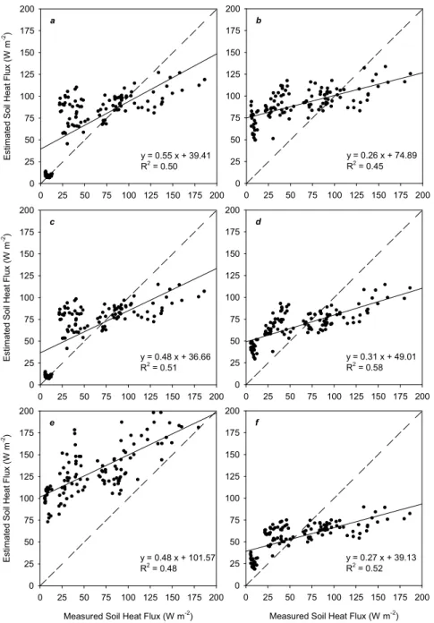
Initially, we analyzed the performance of all original models using data from the three sites, even Rn, G and G/Rn ratio correlated differentially between sites. All models, with exception of Burba et al. (1999), Ma et al. (2001) and Tasumi (2003) to bare soil, had accepted performance with high r and d, but also high RMSE and MAE (Table 3). The Figure 5 represents the relation of G measured in all sites and G estimated by better six performance models.

(9)

0 25 50 75 100 125 150 175 200

E

s

ti

m

at

e

d S

oi

l H

ea

t F

lux

(

W

m

-2)

0 25 50 75 100 125 150 175 200

y = 0.55 x + 39.41 R2_{= 0.50}

a

0 25 50 75 100 125 150 175 200

y = 0.26 x + 74.89 R2 = 0.45 b

0 25 50 75 100 125 150 175 200

E

s

ti

m

at

e

d S

oi

l H

ea

t

F

lux

(

W

m

-2)

0 25 50 75 100 125 150 175 200

y = 0.48 x + 36.66 R2_{= 0.51}

c

0 25 50 75 100 125 150 175 200

y = 0.31 x + 49.01 R2_{= 0.58}

d

Measured Soil Heat Flux (W m-2₎

0 25 50 75 100 125 150 175 200

E

s

ti

m

at

e

d S

oi

l H

ea

t

F

lux

(

W

m

-2)

0 25 50 75 100 125 150 175 200

y = 0.48 x + 101.57 R2 = 0.48 e

Measured Soil Heat Flux (W m-2)

0 25 50 75 100 125 150 175 200

y = 0.27 x + 39.13 R2 = 0.52 f

Figure 5. Relation between soil heat lux measured in all sites and obtained by models proposed by Choudhury et al. (1987) (a); Kustas and Daughtry (1990) (b); Kustas, Daughtry and Oevelen (1993) for LAI < 4 (c); Bastiaanssen (1995) (d); Payero et al., (2001) (e) and Tasumi (2003) for vegetated soil (f).

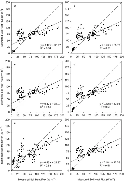
models. The result was the small increase of r of all models with local parameterization, and a considerably increase in d and a decrease in MAE and RMSE of all models (Table 4).

The Bastiaanssen (1995) model is worthy of more attention for the greater r and d and smaller RMSE and MAE. It also should be considered due to large number of biophysical variables in its model formulation (α, LST and NDVI). This model was parameterized to represent a wide type of surface which may be monitored by orbital sensors, such as non-vegetated and vegetated areas, grasslands, forests

or even desert areas and wetlands (Bastiaanssen, 1995). In addition, all these biophysical parameters are strongly correlated with the G/Rn ratio in all sites. The systematic study of the behavior of the G and its parameterization/ calibration in locu should be performed with different

(10)

Authors MAE RMSE d r

Choudhury et al. (1987) 11.05 33.38 0.95 0.71

Jackson et al. (1987) 13.87 36.36 0.94 0.73

Kustas and Daughtry (1990) 28.56 45.65 0.92 0.67

Kustas, Daughtry and Oevelen (1993)

LAI<4 4.31 31.70 0.95 0.71

Kustas, Daughtry and Oevelen (1993)

LAI>4 28.77 51.96 0.76 0.33

Bastiaanssen (1995) 5.70 33.68 0.95 0.76

Burba et al. (1999) 84.15 96.20 0.81 0.33

Payero et al. (2001) 69.16 76.31 0.86 0.69

Ma et al. (2001) 60.66 75.46 0.85 0.33

Tasumi (2003) vegetated soil 6.43 35.28 0.93 0.72

Tasumi (2003) bare soil 62.31 76.77 0.01 -0.06

Ruhoff (2011) 52.35 68.01 0.37 0.71

Table 3 - Mean absolute error (MAE), root mean square error (RMSE), Willmott coeficient (d), and correlation coeficient (r) of original soil heat lux models.

Parameterized Models MAE RMSE d r

 =  × 0.34 ×  −0.5 ×  1.20 31.15 0.95 0.71

 =  × 1.12 × −3.5 ×  3.43 33.29 0.94 0.69

 =  × 0.47 − 0.54 ×  2.03 31.23 0.95 0.72

 =  × 0.34 × −0.50 ×  1.20 31.15 0.95 0.71

 = 0.13 ×  2.05 42.98 0.90 0.33

 =  ×  − 273.16 × 0.0072 + −0.0025 ×  × 1 − 2.11 × _ _1.92 _{29.17 0.96 0.76}

0.17 ×  − 22.5 1.36 42.73 0.90 0.33

 = −7277.0 + 84.82 × 80.92 × 0.0017 ×  − 273.16 + 0.017 ×  0.66 30.61 0.95 0.73

0.17 ×  − 22.50 1.36 42.73 0.90 0.33

 =  × −0.0021 + 0.34 × −0.49 ×  1.12 31.14 0.95 0.71

 = −200.24 ×  − 273.16 ⁄  + 76.0 1.52 45.28 0.88 0.06

 = 0.17 ×  + 12.78 ×  − 273.16 − 424.73 0.64 30.61 0.95 0.73

Table 4 - Reparameterized models and mean absolute error (MAE), root mean square error (RMSE), Willmott coeficient (d), and correlation coeficient (r).

 − 273.16 × −0.0025 + 0.050 ×  × 1 − 2.13 × _{ × } 

 − 273.16 × −5. 10_{+ 0.012 ×  × 1 − 0.14 × }_{ × } 

 − 273.16 × 0.012 + −0.045 ×  × 1 − 1.79 × _{ × } 

 − 273.16 × −0.0025 + 0.050 ×  × 1 − 2.13 × _{ × } 

 − 273.16 × −5. 10_{+ 0.012 ×  × 1 − 0.14 × }_{ × } 

 − 273.16 × 0.012 + −0.045 ×  × 1 − 1.79 × _{ × } 

(13)

(14)

 − 273.16 × −0.0025 + 0.050 ×  × 1 − 2.13 × _{ × } 

 − 273.16 × −5. 10_{+ 0.012 ×  × 1 − 0.14 × }_{ × } 

 − 273.16 × 0.012 + −0.045 ×  × 1 − 1.79 × _{ × } 

(15) As the Bastiaanssen (1995) showed the best performance

to all study areas. We parameterized one model to each site and the result of EMA, RMSE, d and r were 1,18 W m-2_,

(11)

0 25 50 75 100 125 150 175 200

E

s

ti

m

at

e

d S

oi

l H

ea

t F

lux

(

W

m

-2 )

0 25 50 75 100 125 150 175 200

y = 0.47 x + 33.97 R2 = 0.51

a

0 25 50 75 100 125 150 175 200

y = 0.46 x + 35.77 R2 = 0.51

b

0 25 50 75 100 125 150 175 200

E

s

ti

m

at

e

d

S

oi

l

H

ea

t

F

lux

(

W

m

-2)

0 25 50 75 100 125 150 175 200

y = 0.47 x + 33.97 R2 = 0.51

c

0 25 50 75 100 125 150 175 200

y = 0.52 x + 32.04 R2 = 0.58

d

0 25 50 75 100 125 150 175 200

E

s

ti

m

at

e

d

S

oi

l

H

ea

t

F

lux

(

W

m

-2 )

0 25 50 75 100 125 150 175 200

y = 0.53 x + 29.27 R2

= 0.53

e

0 25 50 75 100 125 150 175 200

y = 0.48 x + 33.76 R2

= 0.51

f

Figure 6 - Relation between soil heat lux measured in all sites and obtained by reparameterized models proposed by Choudhury et al. (1987) (a); Kustas and Daughtry (1990) (b); Kustas, Daughtry and Oevelen (1993) for LAI < 4 (c); Bastiaanssen (1995) (d); Payero et al., (2001) (e) and Tasumi (2003) for vegetated soil (f).

4. CONCLUSIONS

The variables obtained by orbital sensors (α, LST, NDVI and LAI) and those obtained in each study area (Rn, G and G/ Rn) showed signiicant inluence of season and study site. In each area, the distinct ecosystem functioning inluenced the different couplings between the variables.

The Bastiaanssen (1995) showed the best performance when it was analyzed for each site separately and for the all tree sites together to obtain a general model.

(12)

5. ACKNOWLEDGMENTS

Funding was provided by the Conselho Nacional de Desenvolvimento Cientíico e Tecnológico (CNPq) and Fundação de Amparo à Pesquisa do Estado de Mato Grosso (FAPEMAT/PRONEX 823971/2009). Additional support was provided by Universidade Federal de Mato Grosso (UFMT).

6. REFERENCES

ALLEN, R.; IRMAK, A.; TREZZA, R.; HENDRICKX, J. M. H.; BASTIAANSSEN. W.; KJAERSGAARD. J. Satellite-based ET estimation in agriculture using SEBAL and METRIC. Hydrological Processes, v.25, p.4011–4027, 2011.

ALLEN, R.; BASTIAANSSEN, W.; WARTES, R.; TASUMI, M.; TREZZA, R. Surface energy balance algorithms for land (SEBAL), Idaho implementation - Advanced training and user’s manual, version 1.0, 2002. 97p.

ALLEN, R.G.; TASUMI, M.; MORSE, A.; TREZZA, R. A Landsat-based energy balance and evapotranspiration model in Western US water rights regulation and planning.

Irrigation and Drainage Systems, v.19, p.251-268, 2005.

ALLEN, R.G.; TASUMI, M.; MORSE, A.; TREZZA, R.; WRIGHT, J.L.; BASTIAANSSEN, W.; KRAMBER, W.; LORITE, I. ROBISON, C. Satellite-based energy balance for Mapping Evapotranspiration with Internalized Calibration (METRIC)—Applications. Journal of Irrigation and

Drainage Engineering, v.133, n.4, p.395-406, 2007.

ARIEIRA, J.; KARSSENBERG, D.; JONG, S.M.; ADDINK, E.A.; COUTO, E.G.; CUNHA, C.N.; SKØIEN, J.O. Integrating field sampling, geostatistics and remote sensing to map wetland vegetation in the Pantanal, Brazil.

Biogeosciences, v.8, p.667–686, 2011.

ARTAXO, P.; OLIVEIRA, P.H.; LARA, L.L.; PAULIQUEVIS, T.M.; RIZZO, L.V.; PIRES JUNIOR, C.; PAIXÃO, M.A.; LONGO, K.M.; FREITAS, S.; CORREIA, A.L. Efeitos climáticos de partículas de aerossóis biogênicos e emitidos em queimadas na Amazônia. Revista Brasileira de

Meteorologia, v.21, n.3a, p.168-189, 2006.

BASTIAANSSEN, W.G.M. Regionalization of surface lux

densities and moisture indicators in composite terrain,

Tese (Ph.D.), Wageningem Agricultural University, Wageningen, Netherlands, 273f., 1995.

BASTIAANSSEN, W.G.M. SEBAL - Based sensible and latent heat luxes in the irrigated Gediz Basin, Turkey. Journal of

Hydrology, v.229, p.87-100, 2000.

BASTIAASSEN, W.G.M.; NOORDMAN, E.J.M.; PELGRUM, H.; DAVIDS, G.; THORESON, B.P.; ALLEN, R.G. SEBAL model with remotely sensed data to improve waterresources

management under actual field conditions. Journal of

Irrigation and Drainage Engineering, v.131, p.85−93, 2005.

BERBET, M.L.C.; COSTA, M.H. Climate change after tropical deforestation: seasonal variability of surface albedo and its effects on precipitation change. Journal of Climate, v.16, p.2099-2104, 2003:

BETTS, R.; SANDERSON, M.; WOODWARD, S. Effect of large-scale Amazon forest degradation on climate and air quality through luxes of carbon dioxide, water, energy, mineral dust and isoprene. Philosophical Transactions of The Royal Society B, v.363, p.1873-1880, 2008.

BEZERRA, B.G.; SILVA, B.B.; FERREIRA, N.J. Estimativa da evapotranspiração real diária utilizando-se imagens digitais TM - Landsat 5. Revista Brasileira de Meteorologia, v.23, n.3, p.305-317, 2008.

BIUDES, M.S.; CAMPELO JÚNIOR, J.H.; NOGUEIRA, J.S.; SANCHES, L. Estimativa do balanço de energia em cambarazal e pastagem no norte do Pantanal pelo método da razão de Bowen. Revista Brasileira de Meteorologia, v.24, n.2, p.135-143, 2009.

BIUDES, M.S.; MACHADO, N.G.; DANELICHEN, V.H.M.; SOUZA, M.C.; VOURLITIS, G.L.; NOGUEIRA, J.S.

International Journal of Biometeorology, 2013. doi:

10.1007/s00484-013-0713-4

BIUDES, M.S; NOGUEIRA, J.S; DALMAGRO, H.J.; MACHADO, N.G.; DANELICHEN, V.H.M.; SOUZA, M.C. Mudança no microclima provocada pela conversão de uma loresta de cambará em pastagem no norte do Pantanal.

Revista de Ciências Agro-Ambientais (Online), v.10,

p.61-68, 2012.

BRÉDA, N. J. J. Ground-based measurements of leaf area index: a review of methods, instruments and current controversies.

Journal of Experimental Botany, v. 54, n. 392, p.

2403-2417. 2003.

BREUER, L.; ECKHARDT, K.; FREDE, H. G. Plant parameter values for models in temperate climates. Ecological

Modelling, v.169, n.2-3, p.237–293, 2003.

BURBA, G.G.; VERMA, S.B.; KIM, J. Surface energy luxes of Phragmites australis in a prairie wetland. Agricultural

and Forest Meteorology, v.94, n.31-51, 1999.

CHOUDHURY, B.L; IDSO, S.B.; REGINATO, R. J. Analysis of an empirical model for soil heat lux under a growing wheat crop for estimating evaporation by an infra-red temperature based energy balance equation. Agricultural and Forest

Meteorology, v.39, p.283-297, 1987.

(13)

COUTINHO, A. C. Precisão posicional dos focos de queimadas no Estado de Mato Grosso. Comunicado Técnico 105, Embrapa. ISSN 1677-8464. Dezembro, 2010. Campinas, SP. CULF, A.D.; FISCH, G.; HODNETT, M.G. The albedo of Amazonian forest and ranchland. Journal of Climate, v.8, n.6, p.1544–1554, 1995.

DAUGHTRY, C.S.; KUSTAS, W.P.; MORAN, M.S.; JACKSON, R.D.; PINTER, J. Spectral estimates of net radiation and soil heat flux. Remote Sensing of Environment, v.32, p.111-124, 1990.

DOUGHTY, C.E.; LOARIE, S.R.; FIELD, C.B., Theoretical Impact of Changing Albedo on Precipitation at the Southernmost Boundary of the ITCZ in South America. Earth Interactions, v.16, p.1–14, 2012.

GHIL, M.; ALLEN, M.R.; DETTINGER, M.D.; IDE, K.; KONDRASHOV, D.; MANN, M.E.; ROBERTSON, A.W.; SAUNDERS, A.; TIAN, Y.; VARADI, F.; YIOU P. Advanced spectral methods for climatic time series. Reviews of Geophysics, v.40, n.1, 2002.

GOLYANDINA, N. and OSIPOVA, E. The “Caterpillar”-SSA

method for analysis of time series with missing values.

Math. Department, St.Petersburg University, Universitetsky av. 28, 198504, St.Petersburg, Petrodvorets, Russia. Feb. 2006. MSC:37M10, 62-07, 60G35. http://www.gistatgroup. com/cat/.

HERRNANCE, J.F.; JACOB, R.W.; BRADLEY, B.A.; MUSTARD, J.F. Extracting phenological signals from multiyear A VHRR NDVI time series: Framework for applying high-order annual splines. IEEE Transactions on

Geoscience and Remote Sensing, v.45, n.10, 2007.

HIRD, J.N.; McDERRNID, G.J. Noise reduction of NDVI time series: An empirical comparison of selected techniques.

Remote Sensing of Environment, v.113, p.248-258, 2009.

HUETE, A.R., K.D.; SHIMABUKURO, Y.E.; RATANA, P.; SALESKA, S.R.; HUTYRA, L.R.; YANG, W.; NEMANI, R. R.; MYNENI, R. Amazon rainforests green-up with sunlight in dry season. Geophysical Research Letters, v.33, p.L06405, 2006.

HUETE, A.R.; DIDAN, K.; MIURA, T.; RODRIGUEZ , E.P.; GAO, X.; FERREIRA, L.G. Overview of the radiometric and biophysical performance of the MODIS vegetation indices. Remote Sensing of Environment, v.83, v.1-2, p.195-213, 2002.

JACKSON, R.D.; MORAN, M.S.; GAY, L.W.; RAYMOND, L.H. Evaluating evaporation from field crops using airborne radiometry and ground-based meteorological data.

Irrigation Sciences, v.8, p.81 – 90, 1987.

KUSTAS, W.; ANDERSON, M. Advances in thermal infrared remote sensing for land surface modeling. Agricultural and

Forest Meteorology, v.149, p.2071−2081, 2009.

KUSTAS, W.P.; DAUGHTRY, C.S.T.. Estimation of the Soil Heat Flux/Net Radiation from Spectral Data. Agriculture

and Forest Meteorology, v.49, p.205–223, 1990.

KUSTAS, W.P.; DAUGHTRY, C.S.T.; VAN OEVELEN, P.J. Analytical Treatment of the Relationships between Soil heat Flux/Net Radiation and Vegetation Indices. Remote Sensing of Environment, v.46, n.3, p.319–330, 1993.

KUSTAS, W.P.; NORMAN, J.M. Evaluation of soil and vegetation heat lux predictions using a simple two-source model with radiometric temperatures for partial canopy cover,

Agricultural and Forest Meteorology, v.94, p.13-29, 1999.

KUSTAS, W.P.; PRUEGER, J.H.; HATFIELD, J.L.; RAMALINGAM, H.; HIPPS, L.E. Variability in soil heat lux from a mesquite dune site. Agricultural and Forest

Meteorology, v.103, n.1, p.249-264, 2000.

MA, Y.; SU, Z.; LI, Z.; KOIKE, T.; MENENTI, M. Determination of regional net radiation and soil heat lux over a heterogeneous landscape of the Tibetan Plateau.

Hydrological Processes, v.16, p.2963–2971, 2001.

MILNE, E.; CERRI, C.E.P.; CARVALHO, J.L.N. Agricultural expansion in the Brazilian state of Mato Grosso; implications for C stocks and greenhouse gas emissions. Environmental

Science and Engeneerig, v.3, p.447-460, 2010.

MU, Q.; HEINSCH, F.A.; ZHAO, M.; RUNNING, S.W. Development of a global evapotranspiration algorithm based on MODIS and global meteorology data. Remote Sensing of Environment, v.111, p.519-536, 2007.

MU. Q.; ZHAO. M.; RUNNING. S.W. Improvements to a

MODIS global terrestrial evapotranspiration algorithm.

Remote Sensing of Environment (2011). Numerical Terradynamic Simulation Group, Department of Ecosystem and Conservation Sciences, The University of Montana, Missoula, MT 59812, USA.

NOSETTO, M., JOBBÁGY, E.; BRIZUELA, A.; JACKSON, R. The hydrologic consequences of land cover change in central Argentina. Agriculture, Ecosystems & Environment, v.154, p.2-11, 2012.

PAYERO, J.; NEALE, C.; WRIGHT, J. Estimating diurnal

variation of soil heat flux for alfalfa and grass,

Proceedings of the 2001 ASAE Annual International Meeting, Sacramento, California. 2001.

PAYERO, J.; NEALE, C.; WRIGHT, J. Estimating soil heat flux for alfalfa and clipped tall fescue grass. Applied Engineering in Agriculture, American Society of

Agricultural Engineers, v.21, n.3, p.401-409, 2005.

RODRIGUES, J.O.; ANDRADE, E.M.; TEIXEIRA, A.S.; SILVA, B.B. Sazonalidade de variáveis biofísicas em regiões semiáridas pelo emprego do sensoriamento remoto.

Engenharia Agrícola, Jaboticabal, v.29, n.3, p.452-465,

(14)

RUHOFF, A. L. Sensoriamento remoto aplicado à estimativa

da evapotranspiração em biomas tropicais. Tese de

doutorado. Universidade federal do Rio Grande do Sul, Instituto de Pesquisas Hidráulicas, Programa de Pós Graduação em Recursos Hídricos e Saneamento Ambiental, Porto Alegre, BR – RS, 2011.

SANTOS, C.A.C.; RAO, T.V.R.; MANZI, A.O. Net radiation estimation under pasture and forest in Rondônia, Brazil, with TM Landsat 5 images. Atmósfera, v.24, n.4, p.435-446, 2011.

SANTOS, T.V.; FONTANA, D.C.; ALVES, R.C.M. Avaliação de fluxos de calor e evapotranspiração pelo modelo SEBAL com uso de dados do sensor ASTER. Pesquisa

Agropecuária Brasileira, v.45, n.5, p.488-496, 2010.

SEPLAN - SECRETARIA DE ESTADO DE PLANEJAMENTO E COORDENAÇÃO GERAL (Mato Grosso) Unidades

climáticas do estado de Mato Grosso. Cuiabá, MT: 2001.

A021p.

SHEIL, D.; MURDIYARSO, D. How forests attract rain: an examination of a new hypothesis. BioScience, v.59, n.4, p.341–347, 2009.

TASUMI, M. Progress in operational estimation of regional

evapotranspiration using satellite imagery. Ph. D.

Dissertation, University of Idaho, Moscow, Idaho. 2003.

TREZZA, R. New Evapotranspiration Crop Coeficients, J.

of Irrig. And Drain. Div. (ASCE), v. 108, p.57-74. 2002.

WANTZEN, K.M.; NUNES DA CUNHA, C.; JUNK, W.J.; GIRARD, P.; ROSSETTO, O.C.; PENHA, J.M.; COUTO, E.G.; BECKER, M.; PRIANTE, G.; TOMAS, W.M.; SANTOS, S.A.; MARTA, J.; DOMINGOS, I.; SONODA, F.; CURVO, M.; CALLIL, C. Towards a sustainable management concept for ecosystem services of the Pantanal wetland. Ecohydrology & Hydrobiology, v.8, n.2-4, p.115-138, 2008.

WILKS, D.S. Statistical methods in the atmospheric sciences. Academic Press, 2011. 676p.

WILLMOTT, C.J.; CKLESON, S.G.; DAVIS, R.E.; FEDDEMA, J.J.; KLINK, K.M.; LEGATES, D.R.; O’DONNELL, J.; ROWE, C.M. Statistics for the evaluation and comparison of models. Journal of Geophysical Research, v.90, n.C5, p.8995-9005, 1985.