INFLUENCE OF MODELS AND SCALES ON THE RANKING OF MULTIATTRIBUTE ALTERNATIVES
Helen M. Moshkovich
1, Luiz Fl´avio Autran Monteiro Gomes
2*,
Alexander I. Mechitov
3and Lu´ıs Alberto Duncan Rangel
4Received September 10, 2009 / Accepted September 19, 2011
ABSTRACT.This paper presents an application of three multiple criteria methods to determining rank of residential real estate options. Methods SAW and TODIM are based on eliciting the decision maker’s preferences (weights and values) directly in a quantitative form while using linear (SAW) and non-linear (TODIM) aggregation functions for alternatives’ evaluation. ZAPROS seeks and uses preferences in an ordinal form as an indirect comparison of trade-offs between criteria. Advantages and disadvantages of different approaches are discussed.
Keywords: Simple Additive Weighting, Verbal Decision Analysis, Multicriteria Decision Aiding.
1 INTRODUCTION
The problem under consideration is the rank of alternatives evaluated against a set of criteria (attributes.) Usually it is assumed that better (more preferable) values against criteria lead to a better overall value of an alternative and to a higher rank in the preference order. To be able to estimate the overall value of each alternative, multiple criteria decision aiding techniques are used to construct an aggregation model on the basis of preference information provided by the decision maker. Rather often such aggregation model is called preference model as it provides a preference structure on the set of alternatives which leads to the sought alternatives’ ranking. Grecoet al.(2008) differentiated two main types of preferential information: direct and indirect. Direct preferential information is used in the traditional aggregation paradigm in the form of scale constant of criteria or aspiration levels or discrimination thresholds or some other parameters necessary for the aggregation model. These parameters are elicited from the decision maker and
*Corresponding author
1School of Business, University of Montevallo, Montevallo, AL, 35115, USA. E-mail: [email protected] 2Ibmec/RJ, Av. Presidente Wilson, 118, Room 1110, 20030-020 Rio de Janeiro, RJ, Brazil. E-mail: [email protected] 3School of Business, University of Montevallo, Montevallo, AL, 35115, USA. E-mail: [email protected] 4UFF/EEIMVR/PUVR, Av. dos Trabalhadores, 420, 27255-125 Volta Redonda, RJ, Brazil.
are then applied in a model to obtain the aggregated value of each alternative. These aggregated values are used to rank alternatives. Many popular multiple criteria methods are based on the paradigm: MAUT (Dyer, 2005), SMART (Edwards & Barron, 1994), AHP (Saaty, 2005) and others (see, e.g. Keeney & Raiffa, 1993; Roy & Bouyssou, 1993; Pomerol & Barba-Romero, 2000; Belton & Stewart, 2002).
The difficulties in assessing these parameters were widely noted (Borcherding et al., 1991; Schoemaker & Waid, 1982; Weber & Borcherding, 1993). Many attempts were made to make it easier for the decision makers to provide this information in an ordinal form. Once obtained, this ordinal information in converted into numbers used in the aggregation model (see,e.g.Cook & Kress, 1992; Kirkwood & Sarin, 1995; Podinovski, 1999; Weber, 1987). The attempts to limit input to the ordinal form usually fail to provide the complete order on the set of alternatives (Shepetukha & Olson, 2001).
Another way to obtain preference information is to use indirect methods of preference elicita-tion, preferably in an ordinal form. According to Grecoet al. (2008) this approach is called the disaggregation (or regression) paradigm where the decision maker provides some holistic pref-erence information (e.g., pairwise comparison of a small number of alternatives from the initial set). These methods are considered to require less cognitive effort from the decision maker. For example, the UTA method (Siskoset al., 2005) seeks additive utility functions from the pref-erence information in the form of alternatives’ ranking carried out by the decision maker. The derived functions may then be used to evaluate other alternatives. There is evidence that compar-ing multiple criteria alternatives consistently is rather difficult and may not be less complicated than providing “weight trade-offs” or “constructing indifference curves for utility functions” in the direct aggregation approach. According to Larichev (1992) it is more comfortable for people to compare alternatives which differ against a relatively small number (2-3) of criteria.
In this paper we compare the results of applying the direct aggregation approach to rank of alter-natives in the residential real estate with the indirect preference elicitation. The direct approach is presented through methods TODIM (Gomes & Lima, 1992; Gomes & Rangel, 2009) and SAW (Simple Additive Weighting) (Keeney & Raiffa, 1993; Vincke, 1989) while the indirect approach is presented through method ZAPROS (Larichev & Moshkovich, 1995, 1997) developed within the framework of Verbal Decision Analysis.
The goal of the research was to analyze the differences in the implementation and the stability of the results obtained through different approaches. The findings are presented and discussed later in the paper.
2 DESCRIPTION OF METHODS
2.1 Problem statement
The SAW Method (Simple Additive Weighting) is one of the more popular and easy to under-stand and use. The approach is based on the Multiple Attribute Value Theory (MAVT) and assumes preferential independence of criteria (see,e.g., Triantaphyllou, 2002). The SAW tech-nique uses a linear additive function to estimate the value of each alternative in the form:
V(aj)= m
X
i=1
wivi j (1)
wherewi is the scale constant of the i-th criterion andvi j is the value of alternativeaj eval-uated by the i-th criterion. The single-attribute values, or utilities vi j reflect how well each alternative does on each criterion. Criterion weights are the relative scale constants of differ-ent criteria leading to the overall valueV(aj)of the alternative. The higher the level of perfor-mance of alternatives according to the criteria with the highest weights, the higher their global value will be.
This approach is widely used in multiple criteria decision making. Main differences in the ap-proaches deal with ways of eliciting weights and single-attribute values (Keeney & Raiffa, 1993; Vincke, 1989). Weights eliciting may follow the reasonably sophisticated approach of swinging weights in SMARTS (Edwards & Barron, 1994), or elaborate weights’ elicitation through a sys-tem of lotteries with trade-offs (Keeney & Raiffa, 1993). In the majority of cases the decision maker evaluates criteria scale constants using some interval or cardinal scales (e.g., if the most important criterion is 100 points, assign appropriate points to other criteria, or use a 5 point scale to assign constant scales to criteria.) The results of such evaluation are normalized, so that the sum of all criterion weightswi is equal to 1.
Single-attribute values for criteria may also be evaluated differently. Rather often quantitative scales are also normalized to produce comparable values. Qualitative scales may be converted into values either directly by the decision maker (e.g., the most preferred value of 1 and the least preferred is 0 and others are assigned values between 1 and 0). Sometimes, as with weights, the decision maker may evaluate them using some cardinal scale (e.g., from 1 to 5). These estimates are then normalized the same way as quantitative scales to produce the required values. In our case, normalization will be used to turn valuesai jinto corresponding valuesvi jas in formula (2). Without loss of generality we assume that in all criteria larger values constitute more preferable estimates.
vi j = ai j n
P
j=1 ai j
Once the weights and single-attribute values are established, each alternative’s “global value” is evaluated according to the additive function (1) and all alternatives are ranked on the basis of these global valuesV(aj), j =1,2, . . . ,n.
2.3 The TODIM Method
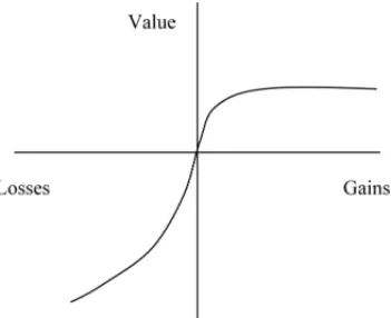
The TODIM method (Gomes & Lima, 1992; Gomes & Maranh˜ao, 2008) is a combination of MAVT approach in the sense that it is based on an additive value function and preferential in-dependence of criteria, but it is close to the, so called, outranking methods (Brans & Mareshal, 1990; Roy & Bouyssou, 1993) as it evaluates overall value of each alternative as a sum of relative “gains” and “losses” of each alternative against all other alternatives in the set.
The initial data for the problem and their normalization intovi j values and criterion weights are defined exactly as in the SAW method. The main difference is how overall alternatives’ values V(aj)are calculated. Computations by TODIM are carried out through the following steps:
2.3.1 Individual criterion weights are recalculated using the most “important” one (criterion cwith the highest weight wc) presenting criterion weights as a proportion of the most important one: for eachwi, 1=1,2, . . . ,m, likewi c=wi/wc.
2.3.2 For each criterioni =1,2, . . . ,mfor each two alternativesaj andak(j,k=1,2, . . . ,n) the “single-attribute dominance”8i(aj,ak)is calculated as:
8i(aj,ak)=
v u u u t
wi c(vi j−vi k) m
P
i=1 wi c
, if (vi j−vi k) >0
0 if (vi j−vi k)=0
−1 θ v u u u t m P i=1
wi c(vi k−vi j)
wi c
, if (vi k−vi j) <0
(3)
Figure 1– Value Function of the TODIM Method (adapted from Gomes & Rangel, 2009).
2.3.3 For each pair of alternatives aj and ak(j,k = 1,2, . . . ,n) the relative “dominance” δ(aj,ak)is calculated as a sum of single-attribute dominance measures8i(aj,ak), i = 1,2, . . . ,m:
δ(aj,ak)= m
X
i=1
8i(aj,ak) (4)
2.3.4 The “global dominance”G(aj)of each alternativeaj, j =1,2, . . .nis calculated as sum of “dominances” over all other alternatives:
G(aj)= m
X
k=1
δ(aj,ak), j =1,2, . . . ,n (5)
2.3.5 The last step normalizes “global dominances” to produce the relative overall valueV(aj) of each alternative using formula:
V(aj)=
G(aj)−minkG(ak)
maxkG(ak)−minkG(ak) (6)
These overall values of the TODIM method, ranging from 0 to 1, are used to rank alterna-tives.
2.4 The ZAPROS Method
2.4.1 Step 1 – Construction of ordinal scales for all criteria
Letλi denote the number of possible levels on the scale of thei-th criterion, then Xi = {xi j} is a set of levels for thei-th criterion rank-ordered from the most preferable to the least prefer-able one. Then we can define the set of all possible alternatives in the criterion space as X =
X1,X2, . . . ,Xm. Then the set of initial alternativesAis a subset ofX.
ZAPROS also assumes that the overall value of each alternative is evaluated by an additive value function as in formula (1) but does not limit the form of value functions for individual criteria to any specific form. The value of the best level on the j-th criterion scale is 1. The value of the least preferable level on this scale is equal to 0:v(xi1)=1,v(xi, γi)=0 fori =1,2, . . .m. The description of alternatives using ordinal scales allows comparison of alternatives according to dominance: alternativeais not less preferable than alternativeb, if for each criterionCi(i =
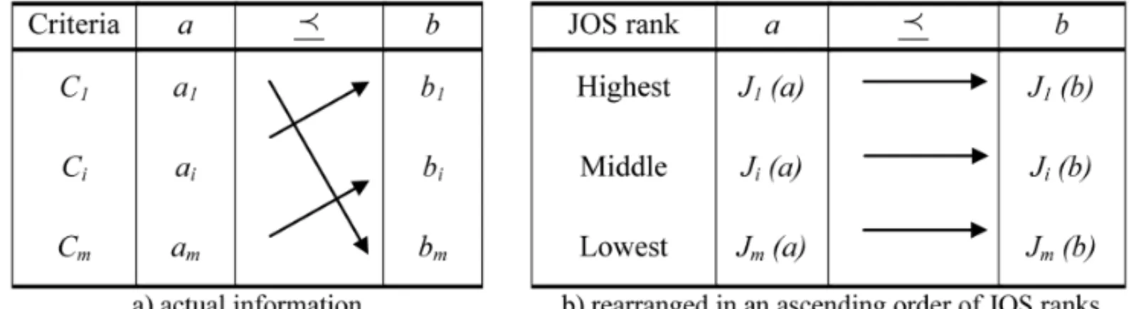
1,2, . . . ,m)estimate ai of alternativea is not less preferable than estimate bi of alternative b (see Fig. 2 below). Usually in real tasks dominance does not lead to any practical order of alternatives. So ZAPROS suggests the next step of the decision maker’s preference elicitation with the goal of constructing a Joint Ordinal Scale (JOS).
Figure 2 – Comparison of real alternatives upon dominance (adapted from Moshkovichet al., 2002).
2.4.2 Step 2 – Construction of the Joint Ordinal Scale (JOS)
The decision-maker is asked to compare pairs of hypothetical alternatives, each with the best levels of attainment on all criteria but one. The number N of these alternatives is given by equation (7):
N =
m
X
i=1
(γj−1)+1 (7)
Figure 3– An example of pairwise comparisons for construction of JOS for criteriaC1andC2.
Comparisons are carried out for all pairs of criteria. On one hand, due to transitivity of pref-erences the number of actual comparisons by the decision maker is much less than the overall number of cells in all these matrices. On another hand, due to transitivity of preferences it is possible to test decision maker’s responses for consistency, thus providing a reliable tested pref-erence structure in the criterion space.
When all necessary comparisons are carried out the criterion value levels starting with the second best, may be ranked. This rank is called the Joint Ordinal Scale (JOS). The place of the criterion value level in this ranking is called JOS rank and is marked asJ(xi j). The smaller the index the better the corresponding criterion level is. Note that all the best value have the same highest rank:
J(x11)= J(x21)= ∙ ∙ ∙ = J(xm1). Thus, we construct a unique ordinal scale for all attributes
with their possible values.
2.4.3 Step 3 – Using JOS for pairwise comparison of alternatives from the set S
Construction of the Joint Ordinal Scale provides a simple rule for comparison of multiattribute alternatives. Each vectora =(a1,a2, . . . ,am)may be rewritten in the form of the rank vector J(a)=(J(a1),J(a2), . . . ,J(am)), where each component is substituted by its JOS rank. The advantage of this presentation is due to the comparability of JOS ranks among criteria. We are not able to comparexi q andxj t but the JOS rank J(xi q)is always comparable with the JOS rankJ(xj t). The rule for comparison the two alternatives on the basis of the JOS is the following: alternativeais not less preferable than alternativeb, if for each component ai of alternativea there may be found a component bj of alternative bsuch that J(ai) J(bj)(see Fig.4for illustration).
The correctness of the rule in case of an additive value function was proven in Larichev & Moshkovich (1995).
To easily implement this rule, it is enough to rearrange elements of each rank vector in an as-cending order:
J1(a) J2(a) ∙ ∙ ∙ Jm(a),
Figure 4– Comparison of real alternatives upon JOS:(J1(x)≺J2(x)≺ ∙ ∙ ∙ ≺ Jm(x))(adapted from
Moshkovichet al., 2002).
3 THE CASE STUDY
3.1 Problem description
The three presented methods were used to compare a set of 15 residential properties available for rent in the city of Volta Redonda in Brazil (Gomes & Rangel, 2009.) Eight most important criteria for property evaluation were established working with the real estate agents and evalu-ators. The analysis in this case study aimed to assisting professionals in the real estate market to evaluate the alternatives more clearly in relation to the evaluation criteria. In other words, by using the results from such analysis realtors were provided a comprehensive way to evaluate properties. All weights used in this case study were provided by these realtors through inter-views. For methods SAW and TODIM qualitative criteria were turned into cardinal scales while quantitative scales were left as they were. For qualitative criteria the TODIM method relies on mapping readings along a qualitative, ordinal scale into corresponding readings along a cardinal scale. By doing this evaluations according to qualitative criteria are transformed into numerical values. For ZAPROS quantitative criteria were divided into a set of levels most appropriate from the point of view of the decision maker were ordered from the least to the most preferred one. The resulting system of criteria is presented in Table 1.
Fifteen alternatives were evaluated against these eight criteria. The result for quantitative scales is presented in Table 2.
3.2 Ranking Alternatives using the SAW Method
A3. Average location 3
A4. Good location 4
A5. Excellent location 5
B. Constructed Area B1. Less than 125 sq.m. sq.m. 3 0.15
B2. Between 125 and 200 sq.m.
B3. Between 200 and 270 sq.m.
B4. Over 270 sq.m.
C. Construction Quality C1. Low standard of finishing 1 2 0.10
C2. Average standard of finishing 2
C3. High standard of finishing 3
D. State of Conservation D1. Bad 1 4 0.20
D2. Average 2
D3. Good 3
D4. Very good 4
E. Number of Garage Spaces E1. No garage space number 1 0.05
E2. One garage space
E3. Two garage spaces
E4. More than2 garage spaces
F. Number of Rooms F1. Four rooms number 2 0.10
F2. Five rooms
F3. Six rooms
F4. Seven rooms
F5. Eight rooms
F6. Nine rooms
G. Attractions G1. Without attractions 0 1 0.05
G2. Backyard or terrace 1
G3. Barbecue 2
G4. Swimming pool 3
G5. Swimming pool, barbecue, etc. 4
H. Security H1. No additional security 0 2 0.10
Table 2– Evaluated alternatives.
Alternatives Criteria
A B C D E F G H
R1 3 290 3 3 1 6 4 0
R2 4 180 2 2 1 4 2 0
R3 3 347 1 2 2 5 1 0
R4 3 124 2 3 2 5 4 0
R5 5 360 3 4 4 9 1 1
R6 2 89 2 3 1 5 1 0
R7 1 85 1 1 1 4 0 1
R8 5 80 2 3 1 6 0 1
R9 2 121 2 3 0 6 0 0
R10 2 120 1 3 1 5 1 0
R11 4 280 2 2 2 7 3 1
R12 1 90 1 1 1 5 2 0
R13 2 160 3 3 2 6 1 1
R14 3 320 3 3 2 8 2 1
R15 4 180 2 4 1 6 1 1
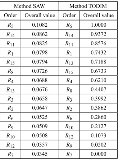
Table 3– Values and rankings of alternatives using methods SAW and TODIM.
Method SAW Method TODIM
Order Overall value Order Overall value
R5 0.1082 R5 1.0000
R14 0.0862 R14 0.9372
R11 0.0825 R11 0.8576
R1 0.0798 R1 0.7432
R15 0.0794 R13 0.7188
R8 0.0726 R15 0.6733
R4 0.0688 R4 0.6210
R13 0.0676 R8 0.4407
R3 0.0658 R3 0.3992
R2 0.0647 R2 0.3862
R6 0.0525 R6 0.2860
R9 0.0509 R10 0.2127
R10 0.0508 R12 0.1073
R12 0.0357 R9 0.0202
The first step is to transform the initial criterion weightswi(i =1,2, . . . ,m)into relative weights using a reference (e.g. the most important) criterion weight. The reference criterion in this problem is the first criterion A and its weight is 0.25. The relative weights are wi1 = wi/w1 i = 1,2, . . . ,m. For criterion A the relative weight is 1(0.25/0.25 = 1), for criterion B it is 0.15/0.25=0.60. Analogously, the relative weights for other criteria are 0.40, 0.80, 0.20, 0.40, 0.20, and 0.40. The sum of all relative weights is equal to 4.
Using the functions8i(Ri,Rk)for each criterioni and for each pair of alternatives j andkare calculated according to formulae (3). Let illustrate the process for alternatives R1 and R2for criterion B.v21=0.103 andv22 =0.064.v21> v22so,
8B(R1,R2)=
s
w21(v21−v22)
Pm i=1wi1
=
r
0.6(0.103−0.064)
4 =0.0764
To evaluate dominance of alternative R1over alternative R2we have to calculate functions8i for each criterion(i =1,2, . . . ,m)and sum up the results to produce a delta function according to formula (4):
δ(R1,R2)= m
X
i=1
8i(R1,R2)=0.0764+(−0.3015)+ ∙ ∙ ∙ + =0.01723
To evaluate the global dominance measure for alternative R1 delta values for all alternatives are summed up according to formula (5): G(R1) = Pn
j=1δ(R1,Rj). The overall value of alternative R1is obtained through normalization of global measures using formula (6). Results for all alternatives are presented in Table 3.
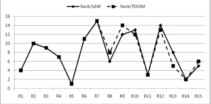
Methods TODIM and SAW use the same formula for scales (criterion values) and the same crite-ria weights, but different aggregation models. The result of the ranking of the same alternatives though is somewhat different for these two methods (see Fig. 5). There are six alternatives with different ranks using these two models:R8,R9,R10,R12,R13, andR15. Without some additional information it is difficult to choose which model best represents the decision maker’s preferences as the assumptions about the decision maker’s preference structure seem to be the same in both methods.
Figure 5– Ranks of real estate alternatives using methods SAW and TODIM.
3.4 Implementation of the ZAPROS method
ZAPROS uses ordinal scales as well as ordinal pairwise comparisons to create the Joint Ordinal Scale (JOS) in a reliable fashion and then uses it to make binary comparisons of the alternatives (thus providing a partial order on the set of 15 alternatives). It is reasonable to expect that alternatives with “reversed” preferences in the previous two models would be left incomparable in ZAPROS as they are evidently close in their overall value.
To obtain the Joint Ordinal Scale (JOS) ordinal scales for all criteria are used (see Table 1). The decision maker is asked to carry out comparison of alternatives differing in values against only two criteria with all other criterion values being at the best possible level. The decision maker is to respond to the following type of questions:
“What would you prefer: an alternative with all the best values but the second best value against criterion A, or an alternative with all the best values but the second best value against criterion B?”
This question may be formulated in a simpler form as follows:
“Do you prefer to have an alternative which has an excellent location and with an area size of 200 to 270 sq. meters or an alternative with a good location and an area size of over 270 sq. meters?”
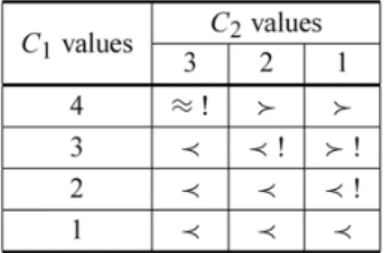
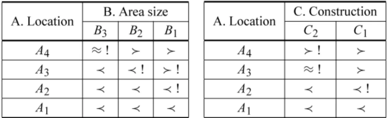
As a result, for each pair of criteria a small matrix of preferences is formed (see an example in Fig. 6). Symbol “≻” means more preferable, “≺” means “less preferable”, and “≈” means “equally preferable”.
Figure 6– Pairwise comparisons near reference point.
transitivity of preferences. In the second matrix, the number of comparisons carried out directly by the decision maker was 3. Some comparisons will be double-checked when comparisons for criteria BandC are formed (see Fig. 7). For example, from Figure 6 we have A4 ≈ B3. This means that preferences of A4compared to criterionCpresented in Figure 6 (A-C) has to be the same for theB3andCpresented in Figure 7. Analogously, A3≈C2, so all conditions forA3in the first matrix has to be correct forC2in matrix in Figure 7. As a result almost all comparisons (marked with the exclamation mark) in the matrix in Figure 7 may be derived from the transitivity relationships and the previous comparisons.
Figure 7– Pairwise comparisons for criteriaBandC.
The transitivity of preferences makes it possible to construct an effective procedure of pairwise comparisons (for more details on the procedure see Larichev & Moshkovich, 1995, 1997). The matrices are constructed for all pairs of criteria, presenting a reliable complete system of pairwise comparisons. This system is used to rank order all criterion values providing ranks for each one of them. The resulting Joint Ordinal Scale is presented in Table 4 (smaller rank presents more preferable criterion values).
To compare 15 alternatives on the basis of JOS we have to substitute each criterion value with the corresponding rankn the JOS, then reorder ranks in an ascending order and compare the resulting alternatives on the basis of a dominance rule.
Table 4– The resulting Joint Ordinal Scale (JOS).
Order in JOS RankJ(xkt)
A5≈B4≈C3≈D4≈ E4≈ F6≈G5≈C2 1
E3≈F3≈G4 2
E2≈F2≈G3 3
A4≈B3≈D3≈G2 4
B2≈ D2 5
A3≈C2 6
H1 7
E1≈G1 8
B1≈C1≈F1 9
A2≈D1 10
A1 11
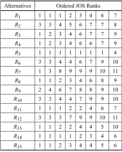
At the next step all alternatives are evaluated through JOS ranks. Let illustrate the process using alternative R1again. ValueA3has a rank of 6 (see Table 4). ValueB4has a rank of 1 and so on. As a result,R1is presented through JOS as (6, 1, 1, 4, 3, 2, 1, 7). The ordered rank presentation of JOS(R1)will be (1, 1, 1, 2, 3, 4, 6, 7) as seen in Table 5.
Table 5– Alternatives evaluated through Ordered JOS Ranks.
Alternatives Ordered JOS Ranks
R1 1 1 1 2 3 4 6 7
R2 3 3 4 5 6 7 7 8
R3 1 2 3 4 6 7 7 9
R4 1 2 3 4 6 6 7 9
R5 1 1 1 1 1 1 1 4
R6 3 3 4 4 6 7 9 10
R7 1 3 8 9 9 9 10 11
R8 1 1 2 3 4 6 8 9
R9 2 4 6 7 8 8 9 10
R10 3 3 4 4 7 9 9 10
R11 1 1 1 2 2 4 6 7
R12 3 3 3 7 9 9 10 11
R13 1 1 2 2 4 4 5 10
R14 1 1 1 1 2 3 4 6
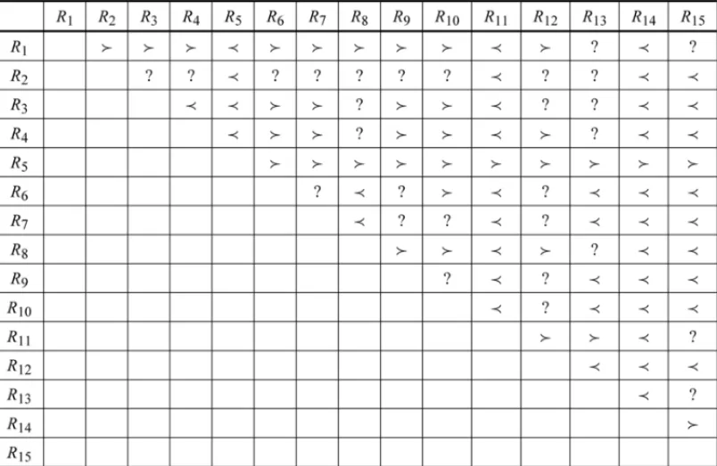
Figure 8– Matrix of pairwise comparisons of alternatives using JOS.
Symbol “?” is used for alternatives left incomparable. Boldfaced cells show the reversed pair-wise comparisons obtained through methods SAW and TODIM. It is reasonable to expect that alternatives with “reversed” preferences in the previous two models would be left incomparable in ZAPROS. Many studies show that stable comparisons of alternatives are provided by different methods only when alternatives are substantially different in value, but it is not the case when alternatives are close in value and should be considered incomparable (or equal) with the used criterion system (Larichevet al., 1995; Olsonet al., 1995).
All cases of reversed preferences in TODIM and SAW were left incomparable when using JOS. There were no reversals with JOS compared to stable preferences in both TODIM and SAW. Some additional alternatives were left incomparable when using JOS due to a limited compen-satory nature of ordinal comparisons. Incomparable alternatives in ZAPROS usually had ranks close to each other in TODIM and SAW.
AlternativeR7has the best value against criterion H (Security) which leads to rank 1 in the JOS representation while many other criterion values are at their lowest level. Thus, the alternative is incomparable with any alternative without the best value against at least one criterion, despite “good” values against all other criteria.
Analysis of incomparable alternatives may flag such situations and be easily resolved through additional pairwise comparisons by the decision maker (see Moshkovich et al., 2002). The comparisons are “goal-oriented”. As with the JOS, the decision maker compares alternatives differing in values against two criteria but there is no requirement that in both alternatives only one value differs from the best level. We asked the decision maker: “Would you prefer an alternative with “no additional security” but with “area size of 200-270 sq. m.” to an alternative with “Doorman and security cameras” but “area size of less than 125 sq. m.”? The question represents a comparison ofB3H1withB1H2. The first combination was preferred to the second which compared alternative R7to all other alternatives as less preferable one.
4 DISCUSSION AND CONCLUSIONS
The presented study confirms the conclusion that it is difficult to ensure reliable evaluation and selection of an appropriate model in a multiple criteria ranking task. Implementation of the same criterion weights and scale transformations for criterion values produced significant differences in the ranking of alternatives when two different methods were used for the aggregation of the preferential information.
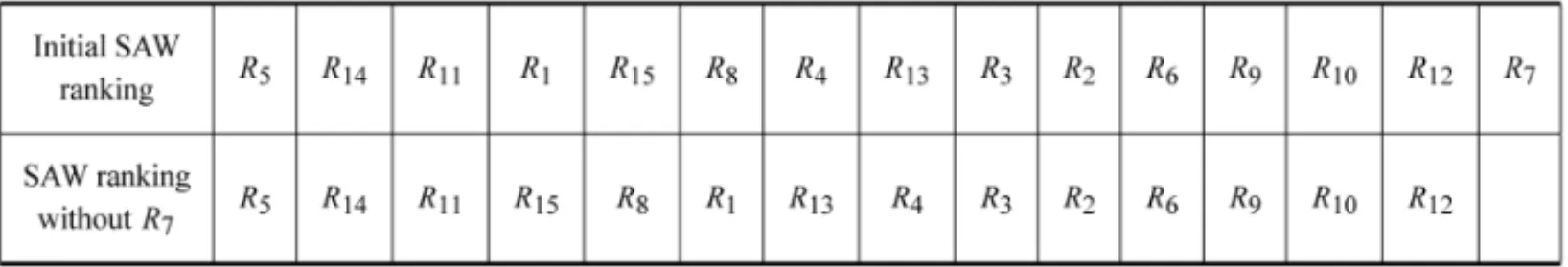
The Simple Additive Weighting model (SAW) produced different ranking for 6 out 15 alter-natives when compared to the ranking obtained through the TODIM method. Both methods assume preferential independence of criteria but TODIM also takes into account relative “gains” and “losses” of one alternative compared to all others. This assumes that the model is dependent on the set of alternatives while the SAW model should be much less dependent on the actual set of alternatives. In general, this is not so as criterion values for both methods are produced from actual scale values in the data set. If we eliminate, for example, alternative R7from the set which was considered by both methods stably the least preferable, there will be no changes in the ranking produced by method TODIM but there will be quite a few changes in the ranking produced with the SAW method as presented below (in Fig. 9):
Figure 9– Outcomes from using the SAW method.
qualitative ones.
The decision maker’s preferences were elicited through pairwise comparison of hypothetical alternatives differing in values against only two criteria with all other values being at their best values. This type of comparison was rather easy for the decision maker and did not re-quire the understanding of the underlying notions or principles except transitivity of preferences. This approach presents an indirect type of preference elicitation. The process though somewhat lengthy, produced reliable information as it was partially double-checked using transitivity re-lationship. This information was used to form the Joint Ordinal Scale which let to for pairwise comparison of the 15 alternatives.
As was expected, the cases of rank reversals using the SAW and the TODIM methods were left incomparable in ZAPROS, while no comparisons contradicted to the ones obtained stably through SAW and TODIM. Due to the limited compensatory nature of ZAPROS some cases were left incomparable, though all these cases dealt with alternatives close in ranking to each other.
The application showed that the ZAPROS method is beneficial to obtaining stable groups of preferred alternatives. In our case, the order from ZAPROS may be viewed as follows:
R5≻R14≻ R11≻(R1,R4,R8,R13,R15)≻ R3≻(R2,R6)≻(R9,R10,R12)≻ R7.
Additional partial orders within the groups are possible. In case ofR7it was easily decided (with one additional question) that it was less preferable than other alternatives despite its best value on security.
Previous studies illustrated that in many cases stable comparisons of alternatives are possible only when the differences in their overall quality are significant. In case of close in value alterna-tives slight changes in procedures and or preferences usually lead to different results. This study supports this idea through the application in a real problem. As in real life situations it is difficult to evaluate a priori how close in value the alternatives are, careful approach to preference elicita-tion is a must. ZAPROS presents one of the more reliable approaches to preference elicitaelicita-tion as it is based on indirect elicitation with the possibility of a feedback on errors in judgment through intransitivity of preferences.
In another application of TODIM to the same data (Gomes & Rangel, 2009) the directly ex-pressed preference was A≻ D≻ B≻C≈F ≈H ≻ E≈G. The most distinction concerned criterion H (Security) which seemed less important to the decision maker when asked through comparison of alternatives than directly. Though usually decision makers have no problems rank ordering criteria by their scale constants, their meaning may not always reflect the actual “trade-off” weights applicable in multiple criteria decision making.
The study showed the attractive features of the ZAPROS method which is based on Verbal De-cision Analysis paradigm and tries to use indirect reliable ordinal judgments from the deDe-cision makers about their preferences. At the same time ZAPROS requires much more time from the decision maker while provides only partial order in alternatives. The decision makers liked SAW and TODIM for their easy application but agreed that they had to rely on the consultants for many decisions about the problem. ZAPROS was attractive due to comfortable information elic-itation process with the feedback (intransitivity of preferences). It provided more assurance for the decision maker in the results of the analysis.
ACKNOWLEDGMENTS
The authors are grateful to the referees for their insightful comments on the first version of this paper. This work was partially supported by CNPq throught Research Projects No. 310603/ 2009-9 and 502711/2009-4.
REFERENCES
[1] BELTON V & STEWART TJ. 2002. Multiple criteria decision analysis: an integrated approach. Massachusetts: Kluwer Academic Publishers.
[2] BOUYSSOUD. 1986. Some remarks on the notion of compensation in MCDM.European Journal of Operational Research,26(1): July, 150–160.
[3] BORCHERDINGK, EPPELT &VONWINTERFELDTD. 1991. Comparison of weighting judgments in multiattribute utility measurement.Management Science,37(2): 1603–1619.
[4] BRANSJP & MARESCHAL B. 1990. The PROM ´ETH ´EE methods for MCDM, the PROMCALC GAIA and BANDADVISER software. In: Readings in Multiple Criteria Decision Aid(edited by C.A. Bana e Costa), chapter 2. Berlin: Springer Verlag, 216–252.
[5] CLEMENR & REILLYT. 2001. Making Hard Decisions with Decision Tools. Pacific Grove, Duxbury.
[6] COOKWD & KRESSM. 1992.Ordinal Information & Preference Structure(Decision Models and Applications). New Jersey: Prentice-Hall, Inc.
[7] DYERJ. 2005. Multiattribute Utility Theory, In:Multiple Criteria Decision Analysis: State of the Art Surveys(edited by J. Figueira, S. Greco & M. Ehrgott), chapter 7, Berlin: Springer Verlag, 265–296.
ria rental evaluation of residential properties.European Journal of Operational Research, 193(1): 204–211.
[12] GRECOS, MOUSSEAUV & SLOWINSKI R. 2008. Ordinal regression revisited: multiple criteria ranking using a set of additive value functions.European Journal of Operational Research,191(2): 415–435.
[13] KAHNEMAND & TVERSKYA. 1979. Prospect theory: An analysis of decision under risk. Econo-metrica,47: 263–292.
[14] KEENEYRL & RAIFFAH. 1993. Decisions with multiple objectives: preferences and value trade-offs. Cambridge: Cambridge University Press.
[15] KIRKWOODCW & SARINRK. 1985. Ranking with partial information: a method and an applica-tion.Operations Research,33: 38–48.
[16] LARICHEVOI. 1992. Cognitive validity in design of decision-aiding techniques.Journal of Multi-Criteria Decision Analysis,1: 127–138.
[17] LARICHEVOI & MOSHKOVICHHM. 1995. ZAPROS-LM – A Method and System for Ordering Multiattribute Alternatives.European Journal of Operational Research,82: 503–521.
[18] LARICHEVOI & MOSHKOVICHHM. 1997.Verbal Decision Analysis for Unstructured Problems. Berlin: Kluwer Academic Publishers.
[19] LARICHEV OI, OLSON DL, MOSHKOVICH HM & MECHITOV AI. 1995. Numericvs.cardinal measurements in multiattribute decision making: (How exact is enough?).Organizational Behavior and Human Decision Processes,64(1): 9–21.
[20] MOSHKOVICHH, MECHITOVA & OLSOND. 2005. Verbal Decision Analysis. In:Multiple Criteria Decision Analysis: State of the Art Surveys(edited by J. Figueira, S. Greco & M. Ehrgott), chapter 15, Berlin: Springer Verlag, 609–640.
[21] MOSHKOVICH HM, MECHITOV AI & OLSON D. 2002. Ordinal Judgments for Comparison of Multiattribute Alternatives.European Journal of Operational Research,137: 625–641.
[22] OLSONDL, MOSHKOVICHHM, SCHELLENBERGERR & MECHITOVAI. 1995. Consistency and Accuracy in Decision Aids: Experiments with Four Multiattribute Systems.Decision Sciences,26: 723–748.
[23] PODINOVSKI V. 1999. A DSS for multiple criteria decision analysis with imprecisely specified trade-offs.European Journal of Operational Research,113: 261–270.
[24] POMEROLJC & BARBA-ROMEROS. 2000.Multicriterion Decision in Management: principles and practice. Boston: Kluwer Academic Publishers.
[26] SAATYTL. 2005. The analytic hierarchy and analytic network processes for the measurement of intangible criteria and for decision-making. In:Multiple Criteria Decision Analysis: State of the Art Surveys(edited by J. Figueira, S. Greco & M. Ehrgott), chapter 9, Berlin: Springer Verlag, 345–408.
[27] SCHOEMAKER PJH & WAID CC. 1982. An experimental comparison of different approaches to determining weights in additive utility models.Management Science,12(2): 182–196.
[28] SISKOS Y, GRIGOROUDISE & MATSATISNISN. 2005. UTA Methods. In: Multiple Criteria De-cision Analysis: State of the Art Surveys(edited by J. Figueira, S. Greco & M. Ehrgott), chapter 8, Berlin: Springer Verlag, 297–344.
[29] SHEPETUKHAY & OLSONDL. 2001. Comparative Analysis of Multiattribute Techniques Based on Cardinal and Ordinal Inputs.Mathematical and Computer Modeling,34: 229–241.
[30] TRIANTAPHYLLOU E. 2002. Multi-Criteria Decision Making Methods: A Comparative Study. Second Edition, Kluwer Academic Publishers.
[31] WEBERM. 1987. Decision Making with Incomplete Information.European Journal of Operational Research,28(1): 1–12.
[32] WEBER M & BORCHERDING M. 1993. Behavioral Influences on weight judgements in